Factor models and variable selection in high-dimensional regression analysis

Alois Kneiplabel=e1]akneip@uni-bonn.de [    Pascal Sardalabel=e2]Pascal.Sarda@math.ups-tlse.fr [ Universität Bonn and Université Paul Sabatier Statistische Abteilung
Department of Economics
 and Hausdorff
Center for Mathematics
Universität Bonn
Adenauerallee 24-26
53113 Bonn
Germany
Institut de Mathématiques
Laboratoire de Statistique
 et Probabilités
Université Paul Sabatier
UMR 5219
118, Route de Narbonne
31062 Toulouse Cedex
France
(2011; 3 2011)
Abstract

The paper considers linear regression problems where the number of predictor variables is possibly larger than the sample size. The basic motivation of the study is to combine the points of view of model selection and functional regression by using a factor approach: it is assumed that the predictor vector can be decomposed into a sum of two uncorrelated random components reflecting common factors and specific variabilities of the explanatory variables. It is shown that the traditional assumption of a sparse vector of parameters is restrictive in this context. Common factors may possess a significant influence on the response variable which cannot be captured by the specific effects of a small number of individual variables. We therefore propose to include principal components as additional explanatory variables in an augmented regression model. We give finite sample inequalities for estimates of these components. It is then shown that model selection procedures can be used to estimate the parameters of the augmented model, and we derive theoretical properties of the estimators. Finite sample performance is illustrated by a simulation study.

62J05,
62H25,
62F12,
Linear regression,
model selection,
functional regression,
factor models,
doi:
10.1214/11-AOS905
keywords:
[class=AMS] .
keywords:
.
volume: 39issue: 5

and

1 Introduction

The starting point of our analysis is a high-dimensional linear regression model of the form

$$Y_{i}=\bolds{\beta}^{T}\mathbf{X}_{i}+\varepsilon_{i},\qquad i=1,\ldots,n,$$ (1)

where $(Y_{i},\mathbf{X}_{i})$, $i=1,\ldots,n$, are i.i.d. random pairs with $Y_{i}\in\mathbb{R}$ and $\mathbf{X}_{i}=(X_{i1},\ldots,X_{ip})^{T}\in\mathbb{R}^{p}$. We will assume without loss of generality that $\mathbb{E}(X_{ij})=0$ for all $j=1,\ldots,p$. Furthermore, $\bolds{\beta}$ is a vector of parameters in $\mathbb{R}^{p}$ and $(\varepsilon_{i})_{i=1,\ldots,n}$ are centered i.i.d. real random variables independent with $\mathbf{X}_{i}$ with $\operatorname{Var}(\varepsilon_{i})=\sigma^{2}$. The dimension $p$ of the vector of parameters is assumed to be typically larger than the sample size $n$.

Roughly speaking, model (1) comprises two main situations which have been considered independently in two separate branches of statistical literature. On one side, there is the situation where $\mathbf{X}_{i}$ represents a (high-dimensional) vector of different predictor variables. Another situation arises when the regressors are $p$ discretizations (e.g., at different observations times) of a same curve. In this case model (1) represents a discrete version of an underlying continuous functional linear model. In the two setups, very different strategies for estimating $\bolds{\beta}$ have been adopted, and underlying structural assumptions seem to be largely incompatible. In this paper we will study similarities and differences of these methodologies, and we will show that a combination of ideas developed in the two settings leads to new estimation procedures which may be useful in a number of important applications.

The first situation is studied in a large literature on model selection in high-dimensional regression. The basic structural assumptions can be described as follows:

  • There is only a relatively small number of predictor variables with $|\beta_{j}|>0$ which have a significant influence on the outcome $Y$. In other words, the set of nonzero coefficients is sparse, $S:=\#\{j|\beta_{j}\neq 0\}\ll p$.

  • The correlations between different explanatory variables $X_{ij}$ and $X_{il}$, $j\neq l$, are “sufficiently” weak.

The most popular procedures to identify and estimate nonzero coefficients $\beta_{j}$ are Lasso and the Dantzig selector. Some important references are Tibshirani (1996), Meinshausen and Bühlmann (2006), Zhao and Yu (2006), van de Geer (2008), Bickel, Ritov and Tsybakov (2009), Candes and Tao (2007) and Koltchinskii (2009). Much work in this domain is based on the assumption that the columns $(X_{1j},\ldots,X_{nj})^{T}$, $j=1,\ldots,p$, of the design matrix are almost orthogonal. For example, Candes and Tao (2007) require that “every set of columns with cardinality less than $S$ approximately behaves like an orthonormal system.” More general conditions have been introduced by Bickel, Ritov and Tsybakov (2009) or Zhou, van de Geer and Bülhmann (2009). The theoretical framework developed in these papers also allows one to study model selection for regressors with substantial amount of correlation, and it provides a basis for the approach presented in our paper.

In sharp contrast, the setup considered in the literature on functional regression rests upon a very different type of structural assumptions. We will consider the simplest case that $X_{ij}=X_{i}(t_{j})$ for random functions $X_{i}\in L^{2}([0,1])$ observed at an equidistant grid $t_{j}=\frac{j}{p}$. Structural assumptions on coefficients and correlations between variables can then be subsumed as follows:

  • $\beta_{j}:=\frac{\beta(t_{j})}{p}$, where $\beta(t)\in L^{2}([0,1])$ is a continuous slope function, and as $p\rightarrow\infty$, $\sum_{j}\beta_{j}X_{ij}=\sum_{j}\frac{\beta(t_{j})}{p}X_{i}(t_{j})\rightarrow\int_{0}^{1}\beta(t)X_{i}(t)\,dt$.

  • There are very high correlations between explanatory variables $X_{ij}=X_{i}(t_{j})$ and $X_{il}=X_{i}(t_{l})$, $j\neq l$. As $p\rightarrow\infty$, $\operatorname{corr}(X_{i}(t_{j}),X_{i}(t_{j+m}))\rightarrow 1$ for any fixed $m$.

Some important applications as well as theoretical results on functional linear regression are, for example, presented in Ramsay and Dalzell (1991), Cardot, Ferraty and Sarda (1999), Cuevas, Febrero and Fraiman (2002), Yao, Müller and Wang (2005), Cai and Hall (2006), Hall and Horowitz (2007), Cardot, Mas and Sarda (2007) and Crambes, Kneip and Sarda (2009). Obviously, in this setup no variable $X_{ij}=X_{i}(t_{j})$ corresponding to a specific observation at grid point $t_{j}$ will possess a particulary high influence on $Y_{i}$, and there will exist a large number of small, but nonzero coefficients $\beta_{j}$ of size proportional to $1/p$. One may argue that dimensionality reduction and therefore some underlying concept of “sparseness” is always necessary when dealing with high-dimensional problems. However, in functional regression sparseness is usually not assumed with respect to the coefficients $\beta_{j}$, but the model is rewritten using a “sparse” expansion of the predictor functions $X_{i}$.

The basic idea relies on the so-called Karhunen–Loève decomposition which provides a decomposition of random functions in terms of functional principal components of the covariance operator of $X_{i}$. In the discretized case analyzed in this paper this amounts to consider an approximation of $X_{i}$ by the principal components of the covariance matrix $\bolds{\Sigma}=\mathbb{E}(\mathbf{X}_{i}\mathbf{X}_{i}^{T})$. In practice, often a small number $k$ of principal components will suffice to achieve a small $L^{2}$-error. An important points is now that even if $p>n$ the eigenvectors corresponding to the leading eigenvalues $\mu_{1},\ldots,\mu_{k}$ of $\bolds{\Sigma}$ can be well estimated by the eigenvectors (estimated principal components) $\widehat{\bolds{\psi}}_{r}$ of the empirical covariance matrix $\widehat{\bolds{\Sigma}}$. This is due to the fact that if the predictors $X_{ij}$ represent discretized values of a continuous functional variable, then for sufficiently small $k$ the eigenvalues $\mu_{1},\ldots,\mu_{k}$ will necessarily be of an order larger than $\frac{p}{\sqrt{n}}$ and will thus exceed the magnitude of purely random components. From a more general point of view the underlying theory will be explained in detail in Section 4.

Based on this insight, the most frequently used approach in functional regression is to approximate $\mathbf{X}_{i}\approx\sum_{r=1}^{k}(\widehat{\bolds{\psi}}^{T}_{r}\mathbf{X}_{i})\widehat{\bolds{\psi}}_{r}$ in terms of the first $k$ estimated principal components $\widehat{\bolds{\psi}}_{1},\ldots,\widehat{\bolds{\psi}}_{k}$, and to rely on the approximate model $Y_{i}\approx\sum_{r=1}^{k}\alpha_{r}\widehat{\bolds{\psi}}{}^{T}_{r}\mathbf{X}_{i}+\varepsilon_{i}$. Here, $k$ serves as smoothing parameter. The new coefficients $\bolds{\alpha}$ are estimated by least squares, and $\widehat{\beta}_{j}=\sum_{r=1}^{k}\widehat{\alpha}_{r}\widehat{\psi}_{rj}$. Resulting rates of convergence are given in Hall and Horowitz (2007).

The above arguments show that a suitable regression analysis will have to take into account the underlying structure of the explanatory variables $X_{ij}$. The basic motivation of this paper now is to combine the points of view of the above branches of literature in order to develop a new approach for model adjustment and variable selection in the practically important situation of strongly correlated regressors. More precisely, we will concentrate on factor models by assuming that the $\mathbf{X}_{i}\in\mathbb{R}^{p}$ can be decomposed in the form

$$\mathbf{X}_{i}=\mathbf{W}_{i}+\mathbf{Z}_{i},\qquad i=1,\ldots,n,$$ (2)

where $\mathbf{W}_{i}$ and $\mathbf{Z}_{i}$ are two uncorrelated random vectors in $\mathbb{R}^{p}$. The random vector $\mathbf{W}_{i}$ is intended to describe high correlations of the $X_{ij}$ while the components $Z_{ij}$, $j=1,\ldots,p$, of $\mathbf{Z}_{i}$ are uncorrelated. This implies that the covariance matrix $\bolds{\Sigma}$ of $\mathbf{X}_{i}$ adopts the decomposition

$$\bolds{\Sigma}=\bolds{\Gamma}+\bolds{\Psi},$$ (3)

where $\bolds{\Gamma}=\mathbb{E}(\mathbf{W}_{i}\mathbf{W}_{i}^{T})$, while $\bolds{\Psi}$ is a diagonal matrix with diagonal entries $\operatorname{var}(Z_{ij})$, $j=1,\ldots,p$.

Note that factor models can be found in any textbook on multivariate analysis and must be seen as one of the major tools in order to analyze samples of high-dimensional vectors. Also recall that a standard factor model is additionally based on the assumption that a finite number $k$ of factors suffices to approximate $\mathbf{W}_{i}$ precisely. This means that the matrix $\bolds{\Gamma}$ only possesses $k$ nonzero eigenvalues. In the following we will more generally assume that a small number of eigenvectors of $\bolds{\Gamma}$ suffices to approximate $\mathbf{W}_{i}$ with high accuracy.

We want to emphasize that the typical structural assumptions to be found in the literature on high-dimensional regression are special cases of (2). If $\mathbf{W}_{i}=0$ and thus $\mathbf{X}_{i}=\mathbf{Z}_{i}$, we are in the situation of uncorrelated regressors which has been widely studied in the context of model selection. On the other hand, $\mathbf{Z}_{i}=0$ and thus $\mathbf{X}_{i}=\mathbf{W}_{i}$ reflect the structural assumption of functional regression.

In this paper we assume that $W_{ij}$ as well as $Z_{ij}$ represent nonnegligible parts of the variance of $X_{ij}$. We believe that this approach may well describe the situation encountered in many relevant applications. Although standard factor models are usually considered in the case $p\ll n$, (2) for large values of $p$ may be of particular interest in time series or spatial analysis. Indeed, factor models for large $p$ with a finite number $k$ of nonzero eigenvalues of $\bolds{\Gamma}$ play an important role in the econometric study of multiple time series and panel data. Some references are Forni and Lippi (1997), Forni et al. (2000), Stock and Watson (2002), Bernanke and Boivin (2003) and Bai (2003, 2009).

Our objective now is to study linear regression (1) with respect to explanatory variables which adopt decomposition (2). Each single variable $X_{ij}$, $j=1,\ldots,p$, then possesses a specific variability induced by $Z_{ij}$ and may thus explain some part of the outcome $Y_{i}$. One will, of course, assume that only few variables have a significant influence on $Y_{i}$ which enforces the use of model selection procedures.

On the other hand, the term $W_{ij}$ represents a common variability. Corresponding principal components quantify a simultaneous variation of many individual regressors. As a consequence, such principal components may possess some additional power for predicting $Y_{i}$ which may go beyond the effects of individual variables. A rigorous discussion will be given in Section 3. We want to note that the concept of “latent variables,” embracing the common influence of a large group of individual variables, plays a prominent role in applied, parametric multivariate analysis.

These arguments motivate the main results of this paper. We propose to use an “augmented” regression model which includes principal components as additional explanatory variables. Established model selection procedures like the Dantzig selector or the Lasso can then be applied to estimate the nonzero coefficients of the augmented model. We then derive theoretical results providing bounds for the accuracy of the resulting estimators.

The paper is organized as follows: in Section 2 we formalize our setup. We show in Section 3 that the traditional sparseness assumption is restrictive and that a valid model may have to include principal components. The augmented model is thus introduced with an estimation procedure. Section 4 deals with the problem how accurately true principal components can be estimated from the sample $\mathbf{X}_{1},\ldots,\mathbf{X}_{n}$. Finite sample inequalities are given, and we show that it is possible to obtain sensible estimates of those components which explain a considerable percentage of the total variance of all $X_{ij}$, $j=1,\ldots,p$. Section 5 focuses on theoretical properties of the augmented model, while in Section 6 we present simulation results illustrating the finite sample performance of our estimators.

2 The setup

We study regression of a response variable $Y_{i}$ on a set of i.i.d. predictors $\mathbf{X}_{i}\in\mathbb{R}^{p}$, $i=1,\ldots,n$, which adopt decomposition (2) with $\mathbb{E}(X_{ij})=\mathbb{E}(W_{ij})=\mathbb{E}(Z_{ij})=0$, $\mathbb{E}(Z_{ij}Z_{ik})=0$, $\mathbb{E}(W_{ij}Z_{il})=0$, $\mathbb{E}(Z_{ij}Z_{ik}Z_{il}Z_{im})=0$ for all $j,k,l,m\in\{1,\ldots,p\}$, $j\notin\{k,l,m\}$. Throughout the following sections we additionally assume that there exist constants $D_{0},D_{3}<\infty$ and $0<D_{1}\leq D_{2}<\infty$ such that with $\sigma_{j}^{2}:=\operatorname{Var}(Z_{ij})$ the following assumption (A.1) is satisfied for all $p$: {longlist}[(A.1)]

$0<D_{1}\leq\sigma_{j}^{2}\leq D_{2},\mathbb{E}(X_{ij}^{2})\leq D_{0},\mathbb{E}(Z_{ij}^{4})\leq D_{3}$ for all $j=1,\ldots,p$. Recall that $\bolds{\Sigma}=\mathbb{E}(\mathbf{X}_{i}\mathbf{X}_{i}^{T})$ is the covariance matrix of $\mathbf{X}_{i}$ with $\bolds{\Sigma}=\bolds{\Gamma}+\bolds{\Psi}$, where $\bolds{\Gamma}=\mathbb{E}(\mathbf{W}_{i}\mathbf{W}_{i}^{T})$ and $\bolds{\Psi}$ is a diagonal matrix with diagonal entries $\sigma^{2}_{j}$, $j=1,\ldots,p$. We denote as $\widehat{\bolds{\Sigma}}=\frac{1}{n}\sum_{i=1}^{n}\mathbf{X}_{i}\mathbf{X}_{i}^{T}$ the empirical covariance matrix based on the sample $\mathbf{X}_{i}$, $i=1,\ldots,n$.

Eigenvalues and eigenvectors of the standardized matrices $\frac{1}{p}\bolds{\Gamma}$ and $\frac{1}{p}\bolds{\Sigma}$ will play a central role. We will use $\lambda_{1}\geq\lambda_{2}\geq\cdots$ and $\mu_{1}\geq\mu_{2}\geq\cdots$ to denote the eigenvalues of $\frac{1}{p}\bolds{\Gamma}$ and $\frac{1}{p}\bolds{\Sigma}$, respectively, while $\bolds{\psi}_{1},\bolds{\psi}_{2},\ldots$ and $\bolds{\delta}_{1},\bolds{\delta}_{2},\ldots$ denote corresponding orthonormal eigenvectors. Note that all eigenvectors of $\frac{1}{p}\bolds{\Sigma}$ and $\bolds{\Sigma}$ (or $\frac{1}{p}\bolds{\Gamma}$ and $\bolds{\Gamma}$) are identical, while eigenvalues differ by the factor $1/p$. Standardization is important to establish convergence results for large $p$, since the largest eigenvalues of $\Sigma$ tend to infinity as $p\rightarrow\infty$.

From a conceptional point of view we will concentrate on the case that $p$ is large compared to $n$. Another crucial, qualitative assumption characterizing our approach is the dimensionality reduction of $\mathbf{W}_{i}$ using a small number $k\ll p$ of eigenvectors (principal components) of $\frac{1}{p}\bolds{\Gamma}$ such that (in a good approximation) $\mathbf{W}_{i}\approx\sum_{r=1}^{k}\xi_{ir}\bolds{\psi}_{r}$. We also assume that $\mathcal{D}_{X}=\frac{1}{p}\sum_{j=1}^{p}\mathbb{E}(X_{ij}^{2})>\mathcal{D}_{W}=\frac{1}{p}\sum_{j=1}^{p}\mathbb{E}(W_{ij}^{2})\gg\frac{1}{p}$. Then all leading principal components of $\frac{1}{p}\bolds{\Gamma}$ corresponding to the $k$ largest eigenvalues explain a considerable percentage of the total variance of $\mathbf{W}_{i}$ and $\mathbf{X}_{i}$.

Indeed, if $\mathbf{W}_{i}=\sum_{r=1}^{k}\xi_{ir}\bolds{\psi}_{r}$, we necessarily have $\lambda_{1}\geq\frac{\mathcal{D}_{W}}{k}\gg\frac{1}{p}$ and $\mu_{1}\geq\lambda_{1}\geq\frac{\mathcal{D}_{W}}{k}\gg\frac{1}{p}$. Then $\operatorname{tr}(\frac{1}{p}\bolds{\Gamma})=\sum_{r=1}^{p}\lambda_{r}=\frac{1}{p}\sum_{j=1}^{p}\mathbb{E}(W_{ij}^{2})$, and the first principal component of $\frac{1}{p}\bolds{\Gamma}$ explains a considerable proportion $\frac{\lambda_{1}}{(1/p)\sum_{j=1}^{p}\mathbb{E}(W_{ij}^{2})}\geq\frac{1}{k}\gg\frac{1}{p}$ of the total variance of $\mathbf{W}_{i}$.

We want to emphasize that this situation is very different from the setup which is usually considered in the literature on the analysis of high-dimensional covariance matrices; see, for example, Bickel and Levina (2008). It is then assumed that the variables of interest are only weakly correlated and that the largest eigenvalue $\mu_{1}$ of the corresponding scaled covariance matrix $\frac{1}{p}\bolds{\Sigma}$ is of order $\frac{1}{p}$. This means that for large $p$ the first principal component only explains a negligible percentage of the total variance of $\mathbf{X}_{i}$, $\frac{\mu_{1}}{(1/p)\sum_{j=1}^{p}\mathbb{E}(X_{ij}^{2})}=O(\frac{1}{p})$. It is well known that in this case no consistent estimates of eigenvalues and principal components can be obtained from an eigen-decomposition of $\frac{1}{p}\widehat{\bolds{\Sigma}}$.

However, we will show in Section 4 that principal components which are able to explain a considerable proportion of total variance can be estimated consistently. These components will be an intrinsic part of the augmented model presented in Section 3.

We will need a further assumption which ensures that all covariances between the different variables are well approximated by their empirical counterparts: {longlist}[(A.2)]

There exists a $C_{0}<\infty$ such that

$\displaystyle\sup_{1\leq j,l\leq p}\Biggl{|}\frac{1}{n}\sum_{i=1}^{n}W_{ij}W_{il}-\operatorname{cov}(W_{ij},W_{il})\Biggr{|}$ $\displaystyle\leq$ $\displaystyle C_{0}\sqrt{\frac{\log p}{n}},$ (4)
$\displaystyle\sup_{1\leq j,l\leq p}\Biggl{|}\frac{1}{n}\sum_{i=1}^{n}Z_{ij}Z_{il}-\operatorname{cov}(Z_{ij},Z_{il})\Biggr{|}$ $\displaystyle\leq$ $\displaystyle C_{0}\sqrt{\frac{\log p}{n}},$ (5)
$\displaystyle\sup_{1\leq j,l\leq p}\Biggl{|}\frac{1}{n}\sum_{i=1}^{n}Z_{ij}W_{il}\Biggr{|}$ $\displaystyle\leq$ $\displaystyle C_{0}\sqrt{\frac{\log p}{n}},$ (6)
$\displaystyle\sup_{1\leq j,l\leq p}\Biggl{|}\frac{1}{n}\sum_{i=1}^{n}X_{ij}X_{il}-\operatorname{cov}(X_{ij},X_{il})\Biggr{|}$ $\displaystyle\leq$ $\displaystyle C_{0}\sqrt{\frac{\log p}{n}}$ (7)

hold simultaneously with probability $A(n,p)>0$, where $A(n,p)\rightarrow 1$ as $n,p\rightarrow\infty$, $\frac{\log p}{n}\rightarrow 0$.

The following proposition provides a general sufficient condition on random vectors for which (A.2) is satisfied provided that the rate of convergence of $\frac{\log p}{n}$ to 0 is sufficiently fast.

Proposition 1

Consider independent and identically distributed random vectors $\mathbf{V}_{i}\in\mathbb{R}^{p}$, $i=1,\ldots,n$, such that for $j=1,\ldots,p$, $\mathbb{E}(V_{ij})=0$ and

$$\mathbb{E}\bigl{(}e^{a|V_{ij}|}\bigr{)}\leq C_{1}$$ (8)

for positive constants $a$ and $C_{1}$ with moreover $\mathbb{E}(V_{ij}^{4})\leq C_{1}$. Then, for any positive constant $C_{0}$ such that $C_{1}^{1/2}\leq\frac{1}{2}\sqrt{\frac{C_{0}n}{\log p}}$ and $C_{1}\leq\frac{1}{8}C_{0}e^{a\sqrt{{C_{0}n}/({\log p})}}\sqrt{\frac{\log p}{n}}$

$\displaystyle P\Biggl{(}\sup_{1\leq j,l\leq p}\Biggl{|}\frac{1}{n}\sum_{i=1}^{n}V_{ij}V_{il}-\operatorname{cov}(V_{ij},V_{il})\Biggr{|}\leq C_{0}\sqrt{\frac{\log p}{n}}\Biggr{)}$
(9)
$\displaystyle\qquad\geq 1-p^{2-C^{2}_{0}/(8(C_{1}+C_{0}^{3/2}/3))}+2p^{2}nC_{1}e^{-({a}/{\sqrt{2}})(C_{0}n/\log p)^{1/4}}.$

Note that as $n,p\rightarrow\infty$ the right-hand side of (1) converges to 1 provided that $C_{0}$ is chosen sufficiently large and that $p/e^{n^{1-\tau}}=O(1)$ for some $4/5<\tau<1$. Therefore, assumption (A.2) is satisfied if the components of the random variables $X_{ij}$ possess some exponential moments. For the specific case of centered normally distributed random variables, a more precise bound in (1) may be obtained using Lemma 2.5 in Zhou, van de Geer and Bülhmann (2009) and large deviations inequalities obtained by Zhou, Lafferty and Wassermn (2008). In this case it may also be shown that for sufficiently large $C_{0}$ events (4)–(7) hold with probability tending to 1 as $p\rightarrow\infty$ without any restriction on the quotient $\log p/n$. Of course, the rate $\sqrt{\frac{\log p}{n}}$ in (4)–(7) depends on the tails of the distributions: it would be possible to replace this rate with a slower one in case of heavier tails than in Proposition 1. Our theoretical results could be modified accordingly.

3 The augmented model

Let us now consider the structural model (2) more closely. It implies that the vector $\mathbf{X}_{i}$ of predictors can be decomposed into two uncorrelated random vectors $\mathbf{W}_{i}$ and $\mathbf{Z}_{i}$. Each of these two components separately may possess a significant influence on the response variable $Y_{i}$. Indeed, if $\mathbf{W}_{i}$ and $\mathbf{Z}_{i}$ were known, a possibly substantial improvement of model (1) would consist in a regression of $Y_{i}$ on the $2p$ variables $\mathbf{W}_{i}$ and $\mathbf{Z}_{i}$

$$Y_{i}=\sum_{j=1}^{p}\beta_{j}^{*}W_{ij}+\sum_{j=1}^{p}\beta_{j}Z_{ij}+\varepsilon_{i},\qquad i=1,\ldots,n,$$ (10)

with different sets of parameters $\beta_{j}^{*}$ and $\beta_{j}$, $j=1,\ldots,p$, for each contributor. We here again assume that $\varepsilon_{i}$, $i=1,\ldots,n$, are centered i.i.d. random variables with $\operatorname{Var}(\varepsilon_{i})=\sigma^{2}$ which are independent of $W_{ij}$ and $Z_{ij}$.

By definition, $W_{ij}$ and $Z_{ij}$ possess substantially different interpretations. $Z_{ij}$ describes the part of $X_{ij}$ which is uncorrelated with all other variables. A nonzero coefficient $\beta_{j}\neq 0$ then means that the variation of $X_{ij}$ has a specific effect on $Y_{i}$. We will of course assume that such nonzero coefficients are sparse, $\sharp\{j|\beta_{j}\neq 0\}\leq S$ for some $S\ll p$. The true variables $Z_{ij}$ are unknown, but with $\beta^{**}_{j}=\beta_{j}^{*}-\beta_{j}$ model (10) can obviously be rewritten in the form

$$Y_{i}=\sum_{j=1}^{p}\beta^{**}_{j}W_{ij}+\sum_{j=1}^{p}\beta_{j}X_{ij}+\varepsilon_{i},\qquad i=1,\ldots,n.$$ (11)

The variables $W_{ij}$ are heavily correlated. It therefore does not make any sense to assume that for some $j\in\{1,\ldots,p\}$ any particular variable $W_{ij}$ possesses a specific influence on the predictor variable. However, the term $\sum_{j=1}^{p}\beta^{**}_{j}W_{ij}$ may represent an important, common effect of all predictor variables. The vectors $\mathbf{W}_{i}$ can obviously be rewritten in terms of principal components. Let us recall that $\lambda_{1}\geq\lambda_{2}\geq\cdots$ denote the eigenvalues of the standardized covariance matrix of $\mathbf{W}_{i}$, $\frac{1}{p}\bolds{\Gamma}=\frac{1}{p}\mathbb{E}(\mathbf{W}_{i}\mathbf{W}_{i}^{T})$ and $\bolds{\psi}_{1},\bolds{\psi}_{2},\ldots$ corresponding orthonormal eigenvectors. We have

$$\mathbf{W}_{i}=\sum_{r=1}^{p}(\bolds{\psi}^{T}_{r}\mathbf{W}_{i})\bolds{\psi}_{r}\quad\mbox{and}\quad\sum_{j=1}^{p}\beta^{**}_{j}W_{ij}=\sum_{r=1}^{p}\alpha_{r}^{*}(\bolds{\psi}^{T}_{r}\mathbf{W}_{i}),$$

where $\alpha_{r}^{*}=\sum_{j=1}^{p}\beta_{j}^{**}\psi_{rj}$. As outlined in the previous sections we now assume that the use of principal components allows for a considerable reduction of dimensionality, and that a small number of leading principal components will suffice to describe the effects of the variable $\mathbf{W}_{i}$. This may be seen as an analogue of the sparseness assumption made for the $Z_{ij}$. More precisely, subsequent analysis will be based on the assumption that the following augmented model holds for some suitable $k\geq 1$:

$$Y_{i}=\sum_{r=1}^{k}\alpha_{r}\xi_{ir}+\sum_{j=1}^{p}\beta_{j}X_{ij}+\varepsilon_{i},$$ (12)

where $\xi_{ir}=\bolds{\psi}^{T}_{r}\mathbf{W}_{i}/\sqrt{p\lambda_{r}}$ and $\alpha_{r}=\sqrt{p\lambda_{r}}\alpha_{r}^{*}$. The use of $\xi_{ir}$ instead of $\bolds{\psi}^{T}_{r}\mathbf{W}_{i}$ is motivated by the fact that $\operatorname{Var}(\bolds{\psi}^{T}_{r}\mathbf{W}_{i})=p\lambda_{r}$, $r=1,\ldots,k$. Therefore the $\xi_{ir}$ are standardized variables with $\operatorname{Var}(\xi_{i1})=\cdots=\operatorname{Var}(\xi_{i1})=1$. Fitting an augmented model requires us to select an appropriate $k$ as well as to determine sensible estimates of $\xi_{i1},\ldots,\xi_{ik}$. Furthermore, model selection procedures like Lasso or Dantzig have to be applied in order to retrieve the nonzero coefficients $\alpha_{r}$, $r=1,\ldots,k$, and $\beta_{j}$, $j=1,\ldots,p$. These issues will be addressed in subsequent sections.

Obviously, the augmented model may be considered as a synthesis of the standard type of models proposed in the literature on functional regression and model selection. It generalizes the classical multivariate linear regression model (1). If a $k$-factor model holds exactly, that is, $\operatorname{rank}(\bolds{\Gamma})=k$, then the only substantial restriction of (10)–(12) consists in the assumption that $Y_{i}$ depends linearly on $W_{i}$ and $Z_{i}$.

We want to emphasize, however, that our analysis does not require the validity of a $k$-factor model. It is only assumed that there exists “some” $Z_{i}$ and $W_{i}$ satisfying our assumptions which lead to (12) for a sparse set of coefficients $\beta_{j}$.

3.1 Identifiability

Let $\bolds{\beta}=(\beta_{1},\ldots,\beta_{p})^{T}$ and $\bolds{\alpha}=(\alpha_{1},\ldots,\alpha_{k})^{T}$. Since $\bolds{\psi}_{r}$, $r=1,\ldots,k$, are eigenvectors of $\bolds{\Gamma}$ we have $\mathbb{E}(\bolds{\psi}^{T}_{r}\mathbf{W}_{i}\bolds{\psi}_{s}^{T}\mathbf{W}_{i})=0$ for all $r,s=1,\ldots,p$, $r\neq s$. By assumption the random vectors $\mathbf{W}_{i}$ and $\mathbf{Z}_{i}$ are uncorrelated, and hence $\mathbb{E}(\bolds{\psi}^{T}_{r}\mathbf{W}_{i}Z_{ij})=0$ for all $r,j=1,\ldots,p$. Furthermore, $\mathbb{E}(Z_{il}Z_{ij})=0$ for all $l\neq j$. If the augmented model (12) holds, some straightforward computations then show that under (A.1) for any alternative set of coefficients $\bolds{\beta}^{*}=(\beta_{1}^{*},\ldots,\beta_{p}^{*})^{T}$, $\bolds{\alpha}^{*}=(\alpha_{1}^{*},\ldots,\alpha_{k}^{*})^{T}$,

$\displaystyle\mathbb{E}\Biggl{(}\Biggl{[}\sum_{r=1}^{k}(\alpha_{r}-\alpha_{r}^{*})\xi_{ir}+\sum_{j=1}^{p}(\beta_{j}-\beta_{j}^{*})X_{ij}\Biggr{]}^{2}\Biggr{)}$
$\displaystyle\qquad\geq\sum_{r=1}^{k}\bigl{(}\alpha_{r}-\alpha_{r}^{*}+\sqrt{p\lambda_{r}}\bolds{\psi}_{r}(\bolds{\beta}-\bolds{\beta}^{*})\bigr{)}^{2}$ (13)
$\displaystyle\qquad\quad{}+D_{1}\|\bolds{\beta}-\bolds{\beta}^{*}\|^{2}_{2}.$

We can conclude that the coefficients $\alpha_{r}$, $r=1,\ldots,k$ and $\beta_{j}$, $j=1,\ldots,p$, in (12) are uniquely determined.

Of course, an inherent difficulty of (12) consists of the fact that it contains the unobserved, “latent” variables $\xi_{ir}=\bolds{\psi}^{T}_{r}\mathbf{W}_{i}/\sqrt{p\lambda_{r}}$. To study this problem, first recall that our setup imposes the decomposition (3) of the covariance matrix $\bolds{\Sigma}$ of $\mathbf{X}_{i}$. If a factor model with $k$ factors holds exactly, then the $\bolds{\Gamma}$ possesses rank $k$. It then follows from well-established results in multivariate analysis that if $k<p/2$ the matrices $\bolds{\Gamma}$ and $\bolds{\Psi}$ are uniquely identified. If $\lambda_{1}>\lambda_{2}>\cdots>\lambda_{k}>0$, then also $\bolds{\psi}_{1},\ldots,\bolds{\psi}_{k}$ are uniquely determined (up to sign) from the structure of $\bolds{\Gamma}$.

However, for large $p$, identification is possible under even more general conditions. It is not necessary that a $k$-factor model holds exactly. We only need an additional assumption on the magnitude of the eigenvalues of $\frac{1}{p}\bolds{\Gamma}$ defining the $k$ principal components of $\mathbf{W}_{i}$ to be considered.

{longlist}

[(A.3)]

The eigenvalues of $\frac{1}{p}\bolds{\Gamma}$ are such that

$$\min_{j,l\leq k,j\neq l}|\lambda_{j}-\lambda_{l}|\geq v(k),\qquad\min_{j\leq k}\lambda_{j}\geq v(k)$$

for some $1\geq v(k)>0$ with $pv(k)>6D_{2}$.

In the following we will qualitatively assume that $k\ll p$ as well as $v(k)\gg 1/p$. More specific assumptions will be made in the sequel. Note that eigenvectors are only unique up to sign changes. In the following we will always assume that the right “versions” are used. This will go without saying.

Theorem 1

Let $\xi_{ir}^{*}:=\frac{\bolds{\delta}^{T}_{r}\mathbf{X}_{i}}{\sqrt{p\mu_{r}}}$ and $\mathbf{P}_{k}=\mathbf{I}_{p}-\sum_{j=1}^{k}\bolds{\psi}_{j}\bolds{\psi}_{j}^{T}$. Under assumptions (A.1) and (A.2) we have for all $r=1,\ldots,k$, $j=1,\ldots,p$ and all $k,p$ satisfying (A.3):

$\displaystyle|\mu_{r}-\lambda_{r}|$ $\displaystyle\leq$ $\displaystyle\frac{D_{2}}{p},$ (14)
$\displaystyle\|\bolds{\psi}_{r}-\bolds{\delta}_{r}\|_{2}$ $\displaystyle\leq$ $\displaystyle\frac{2D_{2}}{pv(k)},$
$\displaystyle\delta_{rj}^{2}$ $\displaystyle\leq$ $\displaystyle\frac{D_{0}}{pv(k)},$
$\displaystyle\mathbb{E}([\xi_{ir}-\xi_{ir}^{*}]^{2})$ $\displaystyle\leq$ $\displaystyle\frac{D_{2}}{p\mu_{r}}+\frac{(8\lambda_{1}+1)D_{2}^{2}}{p^{2}v(k)^{2}\mu_{r}},$
$\displaystyle\mathbb{E}\biggl{(}\biggl{[}\xi_{ir}-\frac{\bolds{\psi}^{T}_{r}\mathbf{X}_{i}}{\sqrt{p\lambda_{r}}}\biggr{]}^{2}\biggr{)}$ $\displaystyle\leq$ $\displaystyle\frac{D_{2}}{p\lambda_{r}},$
$\displaystyle\mathbb{E}\Biggl{(}\Biggl{[}\sum_{r=1}^{k}\alpha_{r}\xi_{ir}-\sum_{r=1}^{k}\alpha_{r}\xi_{ir}^{*}\Biggr{]}^{2}\Biggr{)}$ $\displaystyle\leq$ $\displaystyle k\sum_{r=1}^{k}\alpha_{r}^{2}\biggl{(}\frac{D_{2}}{p\mu_{r}}+\frac{(8\lambda_{1}+1)D_{2}^{2}}{p^{2}v(k)^{2}\mu_{r}}\biggr{)}.$ (17)

For small $p$, standard factor analysis uses special algorithms in order to identify $\bolds{\psi}_{r}$. The theorem tells us that for large $p$ this is unnecessary since then the eigenvectors $\bolds{\delta}_{r}$ of $\frac{1}{p}\bolds{\Sigma}$ provide a good approximation. The predictor $\xi_{ir}^{*}$ of $\xi_{ir}$ possesses an error of order $1/\sqrt{p}$. The error decreases as $p$ increases, and $\xi_{ir}^{*}$ thus yields a good approximation of $\xi_{ir}$ if $p$ is large. Indeed, if $p\rightarrow\infty$ [for fixed $\mu_{r}$, $v(k)$, $D_{1}$ and $D_{2}$] then by (1) we have $\mathbb{E}([\xi_{ir}-\xi_{ir}^{*}]^{2})\rightarrow 0$. Furthermore, by (17) the error in predicting $\sum_{r=1}^{k}\alpha_{r}\xi_{ir}+\sum_{j=1}^{p}\beta_{j}X_{ij}$ by $\sum_{r=1}^{k}\alpha_{r}\xi_{ir}^{*}+\sum_{j=1}^{p}\beta_{j}X_{ij}$ converges to zero as $p\rightarrow\infty$.

A crucial prerequisite for a reasonable analysis of the model is sparseness of the coefficients $\beta_{j}$. Note that if $p$ is large compared to $n$, then by (17) the error in replacing $\xi_{ir}$ by $\xi_{ir}^{*}$ is negligible compared to the estimation error induced by the existence of the error terms $\varepsilon_{i}$. If $k\ll p$ and $\sharp\{j|\beta_{j}\neq 0\}\ll p$, then the true coefficients $\alpha_{r}$ and $\beta_{j}$ provide a sparse solution of the regression problem.

Established theoretical results [see Bickel, Ritov and Tsybakov (2009)] show that under some regularity conditions (validity of the “restricted eigenvalue conditions”) model selection procedures allow to identify such sparse solutions even if there are multiple vectors of coefficients satisfying the normal equations. The latter is of course always the case if $p>n$. Indeed, we will show in the following sections that factors can be consistently estimated from the data, and that a suitable application of Lasso or the Dantzig-selector leads to consistent estimators $\widehat{\alpha}_{r}$, $\widehat{\beta}_{j}$ satisfying $\sup_{r}|\alpha_{r}-\widehat{\alpha}_{r}|\rightarrow_{P}0$, $\sup_{j}|\beta_{j}-\widehat{\beta}_{j}|\rightarrow_{P}0$, as $n,p\rightarrow\infty$.

When replacing $\xi_{ir}$ by $\xi_{ir}^{*}$, there are alternative sets of coefficients leading to the same prediction error as in (17). This is due to the fact that $\xi_{ir}^{*}=\sum_{j=1}^{p}\frac{\delta_{rj}X_{ij}}{\sqrt{p\mu_{r}}}$. However, all these alternative solutions are nonsparse and cannot be identified by Lasso or other procedures. In particular, it is easily seen that

$\displaystyle\sum_{r=1}^{k}\alpha_{r}\xi_{ir}^{*}+\sum_{j=1}^{p}\beta_{j}X_{ij}=\sum_{j=1}^{p}\beta_{j}^{\mathit{LR}}X_{ij}$ (19)
$\displaystyle\eqntext{\displaystyle\mbox{with }\beta^{\mathit{LR}}_{j}:=\beta_{j}+\sum_{r=1}^{k}\alpha_{r}\frac{\delta_{rj}}{\sqrt{p\mu_{r}}}.}$

By (1) all values $\delta_{rj}^{2}$ are of order $1/(pv(k))$. Since $\sum_{j}\delta_{rj}^{2}=1$, this implies that many $\delta_{rj}^{2}$ are nonzero. Therefore, if $\alpha_{r}\neq 0$ for some $r\in\{1,\ldots,k\}$, then $\{j|\beta_{j}^{\mathit{LR}}\neq 0\}$ contains a large number of small, nonzero coefficients and is not at all sparse. If $p$ is large compared to $n$ no known estimation procedure will be able to provide consistent estimates of these coefficients.

Summarizing the above discussion we can conclude:

{longlist}

[(2)]

If the variables $X_{ij}$ are heavily correlated and follow an approximate factor model, then one may reasonably expect substantial effects of the common, joint variation of all variables and, consequently, nonzero coefficients $\beta_{j}^{*}$ and $\alpha_{r}$ in (10) and (12). But then a “bet on sparsity” is unjustifiable when dealing with the standard regression model (1). It follows from (19) that for large $p$ model (1) holds approximately for a nonsparse set of coefficients $\beta_{j}^{\mathit{LR}}$, since many small, nonzero coefficients are necessary in order to capture the effects of the common joint variation.

The augmented model offers a remedy to this problem by pooling possible effects of the joint variation using a small number of additional variables. Together with the familiar assumption of a small number of variables possessing a specific influence, this leads to a sparse model with at most $k+S$ nonzero coefficients which can be recovered from model selection procedures like Lasso or the Dantzig-selector.

In practice, even if (12) only holds approximately, since a too-small value of $k$ has been selected, it may be able to quantify at least some important part of the effects discussed above. Compared to an analysis based on a standard model (1), this may lead to a substantial improvement of model fit as well as to more reliable interpretations of significant variables.

3.2 Estimation

For a pre-specified $k\geq 1$ we now define a procedure for estimating the components of the corresponding augmented model (12) from given data. This obviously specifies suitable procedures for approximating the unknown values $\xi_{ir}$ as well as to apply subsequent model selection procedures in order to retrieve nonzero coefficients $\alpha_{r}$ and $\beta_{j}$, $r=1,\ldots,k$, $j=1,\ldots,p$. A discussion of the choice of $k$ can be found in the next section.

Recall from Theorem 1 that for large $p$ the eigenvectors $\bolds{\psi}_{1},\ldots,\bolds{\psi}_{k}$ of $\frac{1}{p}\bolds{\Gamma}$ are well approximated by the eigenvectors of the standardized covariance matrix $\frac{1}{p}\bolds{\Sigma}$. This motivates us to use the empirical principal components of $\mathbf{X}_{1},\ldots,\mathbf{X}_{n}$ in order to determine estimates of $\bolds{\psi}_{r}$ and $\xi_{ir}$. Theoretical support will be given in the next section. Define $\widehat{\lambda}_{1}\geq\widehat{\lambda}_{2}\geq\cdots$ as the eigenvalues of the standardized empirical covariance matrix $\frac{1}{p}\widehat{\bolds{\Sigma}}=\frac{1}{np}\sum_{i=1}^{n}\mathbf{X}_{i}^{T}\mathbf{X}_{i}$, while $\widehat{\bolds{\psi}}_{1},\widehat{\bolds{\psi}}_{2},\ldots$ are associated orthonormal eigenvectors. We then estimate $\xi_{ir}$ by

$$\widehat{\xi}_{ir}=\widehat{\bolds{\psi}}_{r}^{T}\mathbf{X}_{i}/\sqrt{p\widehat{\lambda}_{r}},\qquad r=1,\ldots,k,i=1,\ldots,n.$$

When replacing $\xi_{ir}$ by $\widehat{\xi}_{ir}$ in (12), a direct application of model selection procedures does not seem to be adequate, since $\widehat{\xi}_{ir}$ and the predictor variables $X_{ij}$ are heavily correlated. We therefore rely on a projected model. Consider the projection matrix on the orthogonal space of the space spanned by the eigenvectors corresponding to the $k$ largest eigenvalues of $\frac{1}{p}\widehat{\bolds{\Sigma}}$

$$\widehat{\mathbf{P}}_{k}=\mathbf{I}_{p}-\sum_{r=1}^{k}\widehat{\bolds{\psi}}_{r}\widehat{\bolds{\psi}}{}^{T}_{r}.$$

Then model (12) can be rewritten for $i=1,\ldots,n$,

$$Y_{i}=\sum_{r=1}^{k}\widetilde{\alpha}_{r}\widehat{\xi}_{ir}+\sum_{j=1}^{p}\widetilde{\beta}_{j}\frac{(\widehat{\mathbf{P}}_{k}\mathbf{X}_{i})_{j}}{(({1/n})\sum_{i=1}^{n}(\widehat{\mathbf{P}}_{k}\mathbf{X}_{i})_{j}^{2})^{1/2}}+\widetilde{\varepsilon}_{i}+\varepsilon_{i},$$ (20)

where $\widetilde{\alpha}_{r}=\alpha_{r}+\sqrt{p\widehat{\lambda}_{r}}\sum_{j=1}^{p}\widehat{\psi}_{rj}\beta_{j}$, $\widetilde{\beta}_{j}=$ $\beta_{j}(\frac{1}{n}\sum_{i=1}^{n}(\widehat{\mathbf{P}}_{k}\mathbf{X}_{i})_{j}^{2})^{1/2}$ and $\widetilde{\varepsilon}_{i}=\sum_{r=1}^{k}\alpha_{r}(\xi_{ir}-\widehat{\xi}_{ir})$. It will be shown in the next section that for large $n$ and $p$ the additional error term $\widetilde{\varepsilon}$ can be assumed to be reasonably small.

In the following we will use $\widetilde{\mathbf{X}}_{i}$ to denote the vectors with entries $\widetilde{X}_{ij}:=\frac{(\widehat{\mathbf{P}}_{k}\mathbf{X}_{i})_{j}}{(({1/n})\sum_{l=1}^{n}(\widehat{\mathbf{P}}_{k}\mathbf{X}_{l})^{2}_{j})^{1/2}}$. Furthermore, consider the $(k+p)$-dimensional vector of predictors $\bolds{\Phi}_{i}:=(\widehat{\xi}_{i1},\ldots,\widehat{\xi}_{ik}$, $\widetilde{X}_{i1},\ldots,\widetilde{X}_{ip})^{T}$. The Gram matrix in model (20) is a block matrix defined as

$$\frac{1}{n}\sum_{i=1}^{n}\bolds{\Phi}_{i}\bolds{\Phi}_{i}^{T}=\pmatrix{\mathbf{I}_{k}&\bolds{0}\vspace*{2pt}\cr\bolds{0}&\displaystyle\frac{1}{n}\sum_{i=1}^{n}\widetilde{\mathbf{X}}_{i}\widetilde{\mathbf{X}}_{i}^{T}},$$

where $\mathbf{I}_{k}$ is the identity matrix of size $k$. Note that the normalization of the predictors in (20) implies that the diagonal elements of the Gram matrix above are equal to 1.

Arguing now that the vector of parameters $\bolds{\theta}:=(\widetilde{\alpha}_{1},\ldots,\widetilde{\alpha}_{k},\widetilde{\beta}_{1},\ldots,\widetilde{\beta}_{p})^{T}$ in model (20) is $(k+S)$-sparse, we may use a selection procedure to recover/estimate the nonnull parameters. In the following we will concentrate on the Lasso estimator introduced in Tibshirani (1996). For a pre-specified parameter $\rho>0$, an estimator $\bolds{\theta}$ is then obtained as

$$\widehat{\bolds{\theta}}=\mathop{\arg\min}_{\widetilde{\bolds{\theta}}\in\mathbb{R}^{k+p}}\frac{1}{n}\|\mathbf{Y}-\bolds{\Phi}\widetilde{\bolds{\theta}}\|_{2}+2\rho\|\widetilde{\bolds{\theta}}\|_{1},$$ (21)

$\bolds{\Phi}$ being the $n\times(k+p)$-dimensional matrix with rows $\bolds{\Phi}_{i}$. We can alternatively use the Dantzig selector introduced in Candes and Tao (2007).

Finally, from $\widehat{\bolds{\theta}}$, we define corresponding estimators for $\alpha_{r}$, $r=1,\ldots,k$, and $\beta_{j}$, $j=1,\ldots,p$, in the unprojected model (12).

$$\widehat{\beta}_{j}=\frac{\hskip 1.5pt\widehat{\widetilde{\beta}}_{j}}{(({1/n})\sum_{i=1}^{n}(\widehat{\mathbf{P}}_{k}\mathbf{X}_{i})_{j}^{2})^{1/2}},\qquad j=1,\ldots,p,$$

and

$$\widehat{\alpha}_{r}=\widehat{\widetilde{\alpha}}_{r}-\sqrt{p\widehat{\lambda}_{r}}\sum_{j=1}^{p}\widehat{\psi}_{rj}\widehat{\beta}_{j},\qquad r=1,\ldots,k.$$

4 High-dimensional factor analysis: Theoretical results

The following theorem shows that principal components which are able to explain a considerable proportion of total variance can be estimated consistently.

For simplicity, we will concentrate on the case that $n$ as well as $p>\sqrt{n}$ are large enough such that {longlist}[(A.4)]

$C_{0}(\log p/n)^{1/2}\geq\frac{D_{0}}{p}$ and $v(k)\geq 6(D_{2}/p+C_{0}(\log p/n)^{1/2})$.

Theorem 2

Under assumptions (A.1)–(A.4) and under events (4)–(7) we have for all $r=1,\ldots,k$ and all $j=1,\ldots,p$,

$\displaystyle|\lambda_{r}-\widehat{\lambda}_{r}|$ $\displaystyle\leq$ $\displaystyle\frac{D_{2}}{p}+C_{0}(\log p/n)^{1/2}$ (22)
$\displaystyle\|\bolds{\psi}_{r}-\widehat{\bolds{\psi}}_{r}\|_{2}$ $\displaystyle\leq$ $\displaystyle 2\frac{{D_{2}}/{p}+C_{0}(\log p/n)^{1/2}}{v(k)},$ (23)
$\displaystyle\psi_{rj}^{2}$ $\displaystyle\leq$ $\displaystyle\frac{D_{0}-D_{1}}{p\lambda_{r}}\leq\frac{D_{0}-D_{1}}{pv(k)},$ (24)
$\displaystyle\widehat{\psi}_{rj}^{2}$ $\displaystyle\leq$ $\displaystyle\frac{D_{0}+C_{0}(\log p/n)^{1/2}}{p\widehat{\lambda}_{r}}$
$\displaystyle\leq$ $\displaystyle\frac{6}{5}\frac{D_{0}+C_{0}(\log p/n)^{1/2}}{pv(k)}.$

Theorem 2 shows that for sufficiently large $p$ ($p>\sqrt{n}$) the eigenvalues and eigenvectors of $\frac{1}{p}\widehat{\bolds{\Sigma}}$ provide reasonable estimates of $\lambda_{r}$ and $\bolds{\psi}_{r}$ for $r=1,\ldots,k$. Quite obviously it is not possible to determine sensible estimates of all $p$ principal components of $\frac{1}{p}\bolds{\Sigma}$. Following the proposition it is required that $\lambda_{r}$ as well as $\mu_{r}$ be of order at least $\sqrt{\frac{\log p}{n}}$. Any smaller component cannot be distinguished from pure “noise” components. Up to the $\log p$-term this corresponds to the results of Hall and Hosseini-Nasab (2006) who study the problem of the number of principal components that can be consistently estimated in a functional principal component analysis.

The above insights are helpful for selecting an appropriate $k$ in a real data application. In tendency, a suitable factor model will incorporate $k$ components which explain a large percentage of the total variance of $\mathbf{X}_{i}$, while $\lambda_{k+1}$ is very small. If for a sample of high-dimensional vectors $\mathbf{X}_{i}$ a principal component analysis leads to the conclusion that the first (or second, third$,\ldots$) principal components explains a large percentage of the total (empirical) variance of the observations, then such a component cannot be generated by “noise” but reflects an underlying structure. In particular, such a component may play a crucial role in modeling a response variable $Y_{i}$ according to an augmented regression model of the form (12).

Bai and Ng (2002) develop criteria of selecting the dimension $k$ in a high-dimensional factor model. They rely on an adaptation of the well-known AIC and BIC procedures in model selection. One possible approach is as follows: Select a maximal possible dimension $k_{\max}$ and estimate $\bar{\sigma}^{2}=\frac{1}{p}\sum_{j=1}^{p}\sigma_{j}^{2}$ by $\widehat{\sigma}^{2}=\frac{1}{np}\sum_{i=1}^{n}\sum_{j=1}^{p}(X_{ij}-\sum_{r=1}^{k_{\max}}(\widehat{\bolds{\psi}}{}^{T}_{r}\mathbf{X}_{i})\widehat{\psi}_{rj})^{2}$. Then determine an estimate $\widehat{k}$ by minimizing

$$\frac{1}{np}\sum_{i=1}^{n}\sum_{j=1}^{p}\Biggl{(}X_{ij}-\sum_{r=1}^{\kappa}(\widehat{\bolds{\psi}}_{r}\mathbf{X}_{i})\widehat{\psi}_{rj}\Biggr{)}^{2}+\kappa\widehat{\sigma}^{2}\biggl{(}\frac{n+p}{np}\biggr{)}\log\min\{n,p\}$$ (26)

over $\kappa=1,\ldots,k_{\max}$. Bai and Ng (2002) show that under some regularity conditions this criterium (as well as a number of alternative versions) provides asymptotically consistent estimates of the true factor dimension $k$ as $n,p\rightarrow\infty$. In our context these regularity conditions are satisfied if (A.1)–(A.4) hold for all $n$ and $p$, $\sup_{j,p}\mathbb{E}(Z_{ij}^{8})<\infty$ and if there exists some $B_{0}>0$ such that $\lambda_{k}\geq B_{0}>0$, for all $n,p$.

Now recall the modified version (20) of the augmented model used in our estimation procedure. The following theorem establishes bounds for the projections $(\widehat{\mathbf{P}}_{k}\mathbf{X}_{i})_{j}$ as well as for the additional error terms $\widetilde{\varepsilon}_{i}$. Let $\mathbf{P}_{k}=\mathbf{I}_{p}-\sum_{j=1}^{k}\bolds{\psi}_{j}\bolds{\psi}_{j}^{T}$ denote the population version of $\widehat{\mathbf{P}}_{k}$.

Theorem 3

Assume (A.1) and (A.2). There then exist constants $M_{1}$, $M_{2}$, $M_{3}<\infty$, such that for all $n,p,k$ satisfying (A.3) and (A.4), all $j,l\in\{1,\ldots,p\}$, $j\neq l$,

$\displaystyle\frac{1}{n}\sum_{i=1}^{n}(\widehat{\mathbf{P}}_{k}\mathbf{X}_{i})_{j}^{2}$ $\displaystyle\geq$ $\displaystyle\sigma_{j}^{2}-M_{1}\frac{kn^{-1/2}\sqrt{\log p}}{v(k)^{1/2}},$ (27)
$\displaystyle\Biggl{|}\frac{1}{n}\sum_{i=1}^{n}(\widehat{\mathbf{P}}_{k}\mathbf{X}_{i})_{j}^{2}-\sigma_{j}^{2}\Biggr{|}$ $\displaystyle\leq$ $\displaystyle\mathbb{E}((\mathbf{P}_{k}\mathbf{W}_{i})_{j}^{2})+M_{2}\frac{kn^{-1/2}\sqrt{\log p}}{v(k)^{3/2}}$ (28)

hold with probability $A(n,p)$, while

$\displaystyle\frac{1}{n}\sum_{i=1}^{n}\widetilde{\varepsilon}_{i}^{2}$ $\displaystyle=$ $\displaystyle\frac{1}{n}\sum_{i=1}^{n}\Biggl{(}\sum_{r=1}^{k}(\widehat{\xi}_{ir}-\xi_{ir})\alpha_{r}\Biggr{)}^{2}$
$\displaystyle\leq$ $\displaystyle\frac{k\alpha^{2}_{\mathrm{sum}}M_{3}}{v(k)^{3}}\biggl{(}\frac{\log p}{n}+\frac{v(k)^{2}}{p}\biggr{)}$

holds with probability at least $A(n,p)-\frac{k}{n}$. Here, $\alpha^{2}_{\mathrm{sum}}=\sum_{r=1}^{k}\alpha_{r}^{2}$.

Note that if $\mathbf{X}_{i}$ satisfies a $k$-dimensional factor model, that is, if the rank of $\frac{1}{p}\bolds{\Gamma}$ is equal to $k$, then $\mathbf{P}_{k}\mathbf{W}_{i}=0$. The theorem then states that for large $n$ and $p$ the projected variables $(\widehat{\mathbf{P}}_{k}\mathbf{X}_{i})_{j}$, $j=1,\ldots,k$, “in average” behave similarly to the specific variables $Z_{ij}$. Variances will be close to $\sigma_{j}^{2}=\operatorname{Var}(Z_{ij})$.

5 Theoretical properties of the augmented model

We come back to model (12). As shown in Section 3.2, the Lasso or the Dantzig selector may be used to determine estimators of the parameters of the model. Identification of sparse solutions as well as consistency of estimators require structural assumptions on the explanatory variables. The weakest assumption on the correlations between different variables seems to be the so-called restricted eigenvalue condition introduced by Bickel, Ritov and Tsybakov (2009); see also Zhou, van de Geer and Bülhmann (2009).

We first provide a theoretical result which shows that for large $n,p$ the design matrix of the projected model (20) satisfies the restricted eigenvalue conditions given in Bickel, Ritov and Tsybakov (2009) with high probability. We will additionally assume that $n,p$ are large enough such that {longlist}[(A.5)]

$D_{1}/2>M_{1}\frac{kn^{-1/2}\sqrt{\log p}}{v(k)^{1/2}}$, where $M_{1}$ is defined as in Theorem 3.

Let $J_{0}$ denote an arbitrary subset of indices, $J_{0}\subset\{1,\ldots,p\}$ with $|J_{0}|\leq k+S$. For a vector $\mathbf{a}\in\mathbb{R}^{k+p}$, let $\mathbf{a}_{J_{0}}$ be the vector in $\mathbb{R}^{k+p}$ which has the same coordinates as $\mathbf{a}$ on $J_{0}$ and zero coordinates on the complement $J_{0}^{c}$ of $J_{0}$. We define in the same way $\mathbf{a}_{J_{0}^{c}}$. Now for $k+S\leq(k+p)/2$ and for an integer $m\geq k+S$, $S+m\leq p$, denote by $J_{m}$ the subset of $\{1,\ldots,k+p\}$ corresponding to $m$ largest in absolute value coordinates of $\mathbf{a}$ outside of $J_{0}$, and define $J_{0,m}:=J_{0}\cup J_{m}$. Furthermore, let $(x)_{+}=\max\{x,0\}$.

Proposition 2

Assume (A.1) and (A.2). There then exists a constant $M_{4}<\infty$, such that for all $n,p,k,S$, $k+S\leq(k+p)/2$, satisfying (A.3)–(A.5), and $c_{0}=1,3$

$\displaystyle\kappa(k+S,k+S,c_{0})$
$\displaystyle\quad:=\min_{J_{0}\subset\{1,\ldots,k+p\}\dvtx|J_{0}|\leq k+S}\min_{\bolds{\Delta}\neq 0\dvtx\|\bolds{\Delta}_{J_{0}^{c}}\|_{1}\leq c_{0}\|\bolds{\Delta}_{J_{0}}\|_{1}}\frac{[\bolds{\Delta}^{T}({1}/{n})\sum_{i=1}^{n}\bolds{\Phi}_{i}\bolds{\Phi}_{i}^{T}\bolds{\Delta}]^{1/2}}{\|\bolds{\Delta}_{J_{0,k+S}}\|_{2}}$
(30)
$\displaystyle\quad\geq\biggl{(}\frac{D_{1}}{D_{0}+C_{0}n^{-1/2}\sqrt{\log p}}-\frac{8(k+S)c_{0}M_{4}k^{2}n^{-1/2}\sqrt{\log p}}{v(k)(D_{1}-M_{1}kv(k)^{1/2}n^{-1/2}\sqrt{\log p})}\biggr{)}_{+}^{{1}/{2}}$
$\displaystyle\quad=:\mathbf{K}_{n,p}(k,S,c_{0})$

holds with probability $A(n,p)$.

Asymptotically, if $n$ and $p$ are large, then $\mathbf{K}_{n,p}(k,S,c_{0})>0$, $c_{0}=1,3$, provided that $k$, $S$ and $1/v(k)$ are sufficiently small compared to $n,p$. In this case the proposition implies that with high probability the restricted eigenvalue condition $\operatorname{RE}(k+S,k+S,c_{0})$ of Bickel, Ritov and Tsybakov (2009) [i.e., $\kappa(k+S,k+S,c_{0})>0$] is satisfied. The same holds for the conditions $\operatorname{RE}(k+S,c_{0})$ which require $\kappa(k+S,c_{0})>0$, where

$\displaystyle\kappa(k+S,c_{0})$
$\displaystyle\qquad:=\min_{J_{0}\subset\{1,\ldots,k+p\}\dvtx|J_{0}|\leq k+S}\min_{\bolds{\Delta}\neq 0\dvtx\|\bolds{\Delta}_{J_{0}^{c}}\|_{1}\leq c_{0}\|\bolds{\Delta}_{J_{0}}\|_{1}}\frac{[\bolds{\Delta}^{T}({1/n})\sum_{i=1}^{n}\bolds{\Phi}_{i}\bolds{\Phi}_{i}^{T}\bolds{\Delta}]^{1/2}}{\|\bolds{\Delta}_{J_{0}}\|_{2}}$
$\displaystyle\qquad\geq\kappa(k+S,k+S,c_{0}).$

The following theorem now provides bounds for the $L^{1}$ estimation error and the $L^{2}$ prediction loss for the Lasso estimator of the coefficients of the augmented model. It generalizes the results of Theorem 7.2 of Bickel, Ritov and Tsybakov (2009) obtained under the standard linear regression model. In our analysis merely the values of $\kappa(k+S,c_{0})$ for $c_{0}=3$ are of interest. However, only slight adaptations of the proofs are necessary in order to derive generalizations of the bounds provided by Bickel, Ritov and Tsybakov (2009) for the Dantzig selector ($c_{0}=1$) and for the $L^{q}$ loss, $1<q\leq 2$. In the latter case, $\kappa(k+S,c_{0})$ has to be replaced by $\kappa(k+S,k+S,c_{0})$. In the following, let $M_{1}$ and $M_{3}$ be defined as in Theorem 3.

Theorem 4

Assume (A.1), (A.2) and suppose that the error terms $\varepsilon_{i}$ in model (12) are independent $\mathcal{N}(0,\sigma^{2})$ random variables with $\sigma^{2}>0$. Now consider the Lasso estimator $\widehat{\bolds{\theta}}$ defined by (21) with

$$\rho=A\sigma\sqrt{\frac{\log(k+p)}{n}}+\frac{M_{5}\alpha_{\mathrm{sum}}}{v(k)^{3/2}}\sqrt{\frac{\log p}{n}},$$

where $A>2\sqrt{2}$, $M_{5}$ is a positive constant and $\alpha_{\mathrm{sum}}=\sum_{r=1}^{k}|\alpha_{r}|$.

If $M_{5}<\infty$ is sufficiently large, then for all $n,p,k$, $k+S\leq(k+p)/2$, satisfying (A.3)–(A.5) as well as $\mathbf{K}_{n,p}(k,S,3)>0$, the following inequalities hold with probability at least $A(n,p)-(p+k)^{-A^{2}/2}$:

$\displaystyle\quad\sum_{r=1}^{k}|\widehat{\alpha}_{r}-\alpha_{r}|$ $\displaystyle\leq$ $\displaystyle\frac{16(k+S)}{\kappa^{2}}$
$\displaystyle{}\times\rho\biggl{(}1+\frac{k(D_{0}+C_{0}n^{-1/2}\sqrt{\log p})^{1/2}}{(D_{1}-M_{1}({kn^{-1/2}\sqrt{\log p}}/{v(k)^{1/2}}))^{1/2}}\biggr{)},$
$\displaystyle\sum_{j=1}^{p}|\widehat{\beta}_{j}-\beta_{j}|$ $\displaystyle\leq$ $\displaystyle\frac{16(k+S)}{\kappa^{2}(D_{1}-M_{1}({kn^{-1/2}\sqrt{\log p}}/{v(k)^{1/2}}))^{1/2}}\rho,$ (32)

where $\kappa=\kappa(k+S,3)$. Moreover,

$\displaystyle\frac{1}{n}\sum_{i=1}^{n}\Biggl{(}\sum_{r=1}^{k}\widehat{\xi}_{ir}\widehat{\alpha}_{r}+\sum_{j=1}^{p}X_{ij}\widehat{\beta}_{j}-\Biggl{(}\sum_{r=1}^{k}\xi_{ir}\alpha_{r}+\sum_{j=1}^{p}X_{ij}\beta_{j}\Biggr{)}\Biggr{)}^{2}$
(33)
$\displaystyle\qquad\leq\frac{32(k+S)}{\kappa^{2}}\rho^{2}+\frac{2k\alpha^{2}_{\mathrm{sum}}M_{3}}{v(k)^{3}}\biggl{(}\frac{\log p}{n}+\frac{v(k)^{2}}{p}\biggr{)}$

holds with probability at least $A(n,p)-(p+k)^{-A^{2}/2}-\frac{k}{n}$.

Of course, the main message of the theorem is asymptotic in nature. If $n,p$ tend to infinity for fixed values of $k$ and $S$, then the $L_{1}$ estimation error and the $L^{2}$ prediction error converge at rates $\sqrt{\log p/n}$ and $\log p/n+1/p$, respectively. For values of $k$ and $S$ tending to infinity as the sample size tends to infinity, the rates are more complicated. In particular, they depend on how fast $v(k)$ converges to zero as $k\rightarrow\infty$. Similar results hold for the estimators based on the Dantzig selector.

Remark 1.

Note that Proposition 2 as well as the results of Theorem 4 heavily depend on the validity of assumption (A.1) and the corresponding value $0<D_{1}\leq\inf_{j}\sigma_{j}^{2}$, where $\sigma_{j}^{2}=\operatorname{var}(Z_{ij})$. It is immediately seen that the smaller the $D_{1}$ the smaller the value of $\kappa(k+S,k+S,c_{0})$ in (2). This means that all variables $X_{ij}=W_{ij}+Z_{ij}$, $j=1,\ldots,p$ have to possess a sufficiently large specific variation which is not shared by other variables. For large $p$ this may be seen as a restrictive assumption. In such a situation one may consider a restricted version of model (12), where variables with extremely small values of $\sigma_{j}^{2}$ are eliminated. But for large $n,p$ we can infer from Theorem 3 that a small value of $\frac{1}{n}\sum_{i=1}^{n}(\widehat{\mathbf{P}}_{k}\mathbf{X}_{i})^{2}_{j}$ indicates that also $\sigma_{j}^{2}$ is small. Hence, an extension of our method consists of introducing some threshold $D_{\mathrm{thresh}}>0$ and discarding all those variables $X_{ij}$, $j\in\{1,\ldots,p\}$, with $\frac{1}{n}\sum_{i=1}^{n}(\widehat{\mathbf{P}}_{k}\mathbf{X}_{i})^{2}_{j}<D_{\mathrm{thresh}}$. A precise analysis is not in the scope of the present paper.

Remark 2.

If $\alpha_{1}=\cdots=\alpha_{k}=0$ the augmented model reduces to the standard linear regression model (1) with a sparse set of coefficients, $\sharp\{j|\beta_{j}\neq 0\}\leq S$ for some $S\leq p$. An application of our estimation procedure is then unnecessary, and coefficients may be estimated by traditional model selection procedures. Bounds on estimation errors can therefore be directly obtained from the results of Bickel, Ritov and Tsybakov (2009), provided that the restricted eigenvalue conditions are satisfied. But in this situation a slight adaptation of the proof of Proposition 2 allows us to establish a result similar to (2) for the standardized variables $X^{*}_{ij}:=X_{ij}/(\frac{1}{n}\sum_{i=1}^{n}X_{ij}^{2})^{1/2}$. Define $\mathbf{X}^{*}$ as the $n\times p$-matrix with generic elements $X_{ij}^{*}$. When assuming (A.1), (A.2) as well as $D_{1}-3C_{0}n^{-1/2}\sqrt{\log p}>0$, then for $S\leq p/2$ the following inequality holds with probability $A(n,p)$:

$\displaystyle\kappa(S,S,c_{0})$
$\displaystyle\qquad:=\min_{J_{0}\subset\{1,\ldots,p\}\dvtx|J_{0}|\leq S}\min_{\bolds{\Delta}\neq 0\dvtx\|\bolds{\Delta}_{J_{0}^{c}}\|_{1}\leq c_{0}\|\bolds{\Delta}_{J_{0}}\|_{1}}\frac{[\bolds{\Delta}^{T}({1/n})\sum_{i=1}^{n}\mathbf{X}^{*}_{i}\mathbf{X}_{i}^{*T}\bolds{\Delta}]^{1/2}}{\|\bolds{\Delta}_{J_{0,S}}\|_{2}}$
$\displaystyle\qquad\geq\biggl{(}\frac{D_{1}}{D_{0}+C_{0}n^{-1/2}\sqrt{\log p}}-\frac{8Sc_{0}C_{0}n^{-1/2}\sqrt{\log p}}{D_{1}-3C_{0}n^{-1/2}\sqrt{\log p}}\biggr{)}_{+}^{1/2},$

where $c_{0}=1,3$. Recall, however, from the discussion in Section 3.1 that $\alpha_{1}=\cdots=\alpha_{k}=0$ is a restrictive condition in the context of highly correlated regressors.

6 Simulation study

In this section we study the finite sample performance of the estimators discussed in the proceeding sections. We consider a factor model with $k=2$ factors. The first factor is $\psi_{1j}=1/\sqrt{p}$, $j=1,\ldots,p$, while the second factor is given by $\psi_{2j}=1/\sqrt{p}$, $j=1,\ldots,p/2$, and $\psi_{2j}=-1/\sqrt{p}$, $j=p/2+1,\ldots,p$. For different values of $n,p,\alpha_{1},\alpha_{2}$ and $0<\lambda_{1}<1,0<\lambda_{2}<1$ observations $(\mathbf{X}_{i},Y_{i})$ with $\operatorname{var}(X_{ij})=1$, $j=1,\ldots,p$, are generated according to the model

$\displaystyle X_{ij}$ $\displaystyle=$ $\displaystyle\sqrt{p\lambda_{1}}\xi_{i1}\psi_{1j}+\sqrt{p\lambda_{2}}\xi_{i2}\psi_{2j}+Z_{ij},$ (35)
$\displaystyle Y_{i}$ $\displaystyle=$ $\displaystyle\alpha_{1}\xi_{i1}+\alpha_{2}\xi_{i1}+\sum_{j=1}^{p}\beta_{j}X_{ij}+\varepsilon_{i},$ (36)

where $\xi_{ir}\sim N(0,1)$, $r=1,2$, $Z_{ij}\sim N(0,1-\lambda_{1}-\lambda_{2})$, and $\varepsilon_{i}\sim N(0,\sigma^{2})$ are independent variables. Our study is based on $S=\sharp\{j|\beta_{j}\neq 0\}=4$ nonzero $\beta$-coefficients whose values are $\beta_{10}=1$, $\beta_{20}=0.3$, $\beta_{21}=-0.3$ and $\beta_{40}=-1$, while the error variance is set to $\sigma^{2}=0.1$.

The parameters of the augmented model with $k=2$ are estimated by using the Lasso-based estimation procedure described in Section 3.2. The behavior of the estimates is compared to the Lasso estimates of the coefficients of a standard regression model (1). All results reported in this section are obtained by applying the LARS-package by Hastie and Efron implemented in R. All tables are based on 1,000 repetitions of the simulation experiments. The corresponding R-code can be obtained from the authors upon request.

Figure 1 and Table 1 refer to the situation with $\lambda_{1}=0.4$, $\lambda_{2}=0.2$, $\alpha_{1}=1$ and $\alpha_{2}=-0.5$. We then have $\operatorname{var}(X_{ij})=1$, $j=1,\ldots,p$, while the first and second factor explain 40% and 20% of the total variance of $X_{ij}$, respectively.

Refer to caption
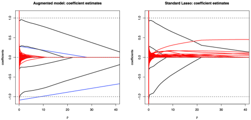
Figure 1: Paths of Lasso estimates for the augmented model (left panel) and the standard linear model (right panel) in dependence of $\rho$; black—estimates of nonzero $\beta_{j}$; red—estimates of coefficients with $\beta_{j}=0$; blue—$\widehat{\widetilde{\alpha}}_{r}$.
Table 1: Estimation errors for different sample sizes ($\lambda_{1}=0.4,\lambda_{2}=0.2,\alpha_{1}=1,\alpha_{2}=-0.5$)
Sample sizes Parameter estimates Prediction
$\bolds{n}$ $\bolds{p}$ $\bolds{\sum|\widehat{\alpha}_{r}-\alpha_{r}|}$ $\bolds{\sum|\widehat{\beta}_{r}-\beta_{r}|}$ Opt. $\bolds{\rho}$ Sample Exact Opt. $\bolds{\rho}$ $\bolds{C_{P}}$
Lasso applied to augmented model:
  00,50 00,50 0.3334 0.8389 $4.53$ 0.0498 0.1004 $1.76$ $1.55$
100 0,100 0.2500 0.5774 $6.84$ 0.0328 0.0480 $3.50$ $3.29$
250 0,250 0.1602 0.3752 $12.27$ 0.0167 0.0199 $7.55$ $7.22$
500 0,500 0.1150 0.2752 $18.99$ 0.0096 0.0106 $12.66$ $12.21$
5,000 0,100 0.0378 0.0733 $48.33$ 0.0152 0.0154 $27.48$ $26.74$
100 2,000 0.2741 0.8664 $10.58$ 0.0420 0.0651 $5.42$ $5.24$
$\bolds{n}$ $\bolds{p}$ $\bolds{\sum|\widehat{\beta}_{r}-\beta_{r}^{\mathit{LR}}|}$ $\bolds{\sum|\widehat{\beta}_{r}-\beta_{r}|}$ Sample Exact Opt. $\bolds{\rho}$
Lasso applied to standard linear regression model:
  00,50 00,50 2.2597 1.8403 0.0521 0.1370 $0.92$
100 0,100 2.2898 1.9090 0.0415 0.0725 $1.90$
250 0,250 2.3653 1.7661 0.0257 0.0345 $4.12$
500 0,500 2.4716 1.7104 0.0174 0.0207 $6.87$
5,000 0,100 0.5376 1.5492 0.0161 0.0168 $10.14$
100 2,000 3.7571 2.2954 0.0523 0.1038 $3.17$

Figure 1 shows estimation results of one typical simulation with $n=p=100$. The left panel contains the parameter estimates for the augmented model. The paths of estimated coefficients $\widehat{\beta}_{j}$ for the 4 significant variables (black lines), the 96 variables with $\beta_{j}=0$ (red lines), as well as of the untransformed estimates $\widehat{\widetilde{\alpha}}_{r}$ (blue lines) of $\alpha_{r}$, $r=1,2$, are plotted as a function of $\rho$. The four significant coefficients as well as $\alpha_{1}$ and $\alpha_{2}$ can immediately been identified in the figure. The right panel shows a corresponding plot of estimated coefficients when Lasso is directly applied to the standard regression model (1). As has to be expected by (19) the necessity of compensating the effects of $\alpha_{1},\alpha_{2}$ by a large number of small, nonzero coefficients generates a general “noise level” which makes it difficult to identify the four significant variables in (36). The penalties $\rho$ in the figure as well as in subsequent tables have to be interpreted in terms of the scaling used by the LARS-algorithm and have to be multiplied with $2/n$ in order to correspond to the standardization used in the proceeding sections.

The upper part of Table 1 provides simulation results with respect to the augmented model for different sample sizes $n$ and $p$. In order to access the quality of parameter estimates we evaluate $\sum_{r=1}^{2}|\widehat{\alpha}_{r}-\alpha_{r}|$ as well as $\sum_{j=1}^{p}|\widehat{\beta}_{r}-\beta_{r}|$ at the optimal value of $\rho$, where the minimum of $\sum_{r=1}^{2}|\widehat{\alpha}_{r}-\alpha_{r}|+\sum_{j=1}^{p}|\widehat{\beta}_{r}-\beta_{r}|$ is obtained. Moreover, we record the value of $\rho$ where the minimal sample prediction error

$$\frac{1}{n}\sum_{i=1}^{n}\Biggl{(}\sum_{r=1}^{2}\alpha_{r}\xi_{ir}+\sum_{j=1}^{p}\beta_{j}X_{ij}-\Biggl{(}\sum_{r=1}^{2}\widehat{\alpha}_{r}\widehat{\xi}_{ir}+\sum_{j=1}^{p}\widehat{\beta}_{j}X_{ij}\Biggr{)}\Biggr{)}^{2}$$ (37)

ia attained. For the same value $\rho$ we also determine the exact prediction error

$$\quad\mathbb{E}\Biggl{(}\sum_{r=1}^{2}\alpha_{r}\xi_{n+1,r}+\sum_{j=1}^{p}\beta_{j}X_{n+1,j}-\Biggl{(}\sum_{r=1}^{2}\widehat{\alpha}_{r}\widehat{\xi}_{n+1,r}+\sum_{j=1}^{p}\widehat{\beta}_{j}X_{n+1,j}\Biggr{)}\Biggr{)}^{2}$$ (38)

for a new observation $\mathbf{X}_{n+1}$ independent of $X_{1},\ldots,X_{n}$. The columns of Table 1 report the average values of the corresponding quantities over the 1,000 replications. To get some insight into a practical choice of the penalty, the last column additionally yields the average value of the parameters $\rho$ minimizing the $C_{P}$-statistics. $C_{P}$ is computed by using the R-routine “summary.lars” and plugging in the true error variance $\sigma^{2}=0.1$. We see that in all situations the average value of $\rho$ minimizing $C_{P}$ is very close to the average $\rho$ providing the smallest prediction error. The penalties for optimal parameter estimation are, of course, larger.

It is immediately seen that the quality of estimates considerably increases when going from $n=p=50$ to $n=p=500$. An interesting result consists of the fact that the prediction error is smaller for $n=p=500$ than for $n=5\mbox{,}000$, $p=100$. This may be interpreted as a consequence of (17).

The lower part of Table 1 provides corresponding simulation results with respect to Lasso estimates based on the standard regression model. In addition to the minimal error $\sum_{r=1}^{p}|\widehat{\beta}_{r}-\beta_{r}|$ in estimating the parameters $\beta_{j}$ of (36) we present the minimal $L_{1}$-distance $\sum_{r=1}^{p}|\widehat{\beta}_{r}-\beta_{r}^{\mathit{LR}}|$, where $\beta_{1}^{\mathit{LR}},\ldots,\beta_{p}^{\mathit{LR}}$ is the (nonsparse) set of parameters minimizing the population prediction error. Sample and exact prediction errors are obtained by straightforward modifications of (37) and (38). Quite obviously, no reasonable parameter estimates are obtained in the cases with $p\geq n$. Only for $n=5\mbox{,}000$, $p=100$, the table indicates a comparably small error $\sum_{r=1}^{p}|\widehat{\beta}_{r}-\beta_{r}^{\mathit{LR}}|$. The prediction error shows a somewhat better behavior. It is, however, always larger than the prediction error of the augmented model. The relative difference increases with $p$.

It was mentioned in Section 4 that a suitable criterion to estimate the dimension $k$ of an approximate factor model consists in minimizing (26). This criterion proved to work well in our simulation study. Recall that the true factor dimension is $k=2$. For $n=p=50$ the average value of the estimate $\widehat{k}$ determined by (26) is 2.64. In all other situations reported in Table 1 an estimate $\widehat{k}=2$ is obtained in each of the 1,000 replications.

Table 2: Estimation errors under different setups ($n=100,p=250$)
Parameter estimates Prediction
$\bolds{\lambda_{1}}$ $\bolds{\lambda_{2}}$ $\bolds{\alpha_{1}}$ $\bolds{\alpha_{2}}$ $\bolds{\sum|\widehat{\alpha}_{r}-\alpha_{r}|}$ $\bolds{\sum|\widehat{\beta}_{r}-\beta_{r}|}$ Opt. $\bolds{\rho}$ Sample Exact Opt. $\bolds{\rho}$
Lasso applied to augmented model:
0.06 $0.03$ 1 $-0.5$ 0.3191 0.6104 $10.37$ 0.0670 0.2259 2.46
0.2 $0.1$ 1 $-0.5$ 0.2529 0.5335 $8.19$ 0.0414 0.0727 3.92
0.4 $0.2$ 1 $-0.5$ 0.2500 0.6498 $7.86$ 0.0319 0.0454 4.35
0.6 $0.3$ 1 $-0.5$ 0.2866 1.1683 $8.46$ 0.0273 0.0350 4.56
0.06 $0.03$ 0 00 0.0908 0.4238 $7.42$ 0.0257 0.0311 4.62
0.2 $0.1$ 0 00 0.1044 0.4788 $7.64$ 0.0257 0.0316 4.69
0.4 $0.2$ 0 00 0.1192 0.6400 $7.84$ 0.0250 0.0314 4.74
0.6 $0.3$ 0 00 0.1825 1.1745 $8.78$ 0.0221 0.0276 5.13
$\bolds{\lambda_{1}}$ $\bolds{\lambda_{2}}$ $\bolds{\alpha_{1}}$ $\bolds{\alpha_{2}}$ $\bolds{\sum|\widehat{\beta}_{r}-\beta_{r}^{\mathit{LR}}|}$ $\bolds{\sum|\widehat{\beta}_{r}-\beta_{r}|}$ Sample Exact Opt. $\bolds{\rho}$
Lasso applied to standard linear regression model:
0.06 $0.03$ 1 $-0.5$ 5.0599 1.9673 0.0777 0.3758 1.95
0.2 $0.1$ 1 $-0.5$ 3.4465 2.3662 0.0583 0.1403 2.63
0.4 $0.2$ 1 $-0.5$ 2.9215 2.0191 0.0425 0.0721 2.45
0.6 $0.3$ 1 $-0.5$ 3.2014 2.2246 0.0277 0.0387 1.47
0.06 $0.03$ 0 00 0.4259 0.4259 0.0216 0.0285 4.80
0.2 $0.1$ 0 00 0.4955 0.4955 0.0222 0.0295 4.24
0.4 $0.2$ 0 00 0.6580 0.6580 0.0228 0.0303 3.17
0.6 $0.3$ 0 00 1.1990 1.1990 0.0215 0.0283 1.66

Finally, Table 2 contains simulations results for $n=100$, $p=250$, and different values of $\lambda_{1},\lambda_{2},\alpha_{1},\alpha_{2}$. All columns have to be interpreted similar to those of Table 1. For $\alpha_{1}=1,\alpha_{2}=-0.5$ suitable parameter estimates can obviously only been determined by applying the augmented model. For $\alpha_{1}=\alpha_{2}=0$ model (36) reduces to a sparse, standard linear regression model. It is then clearly unnecessary to apply the augmented model. Both methods then lead to roughly equivalent parameter estimates.

We want to emphasize that $\lambda_{1}=0.06$, $\lambda_{2}=0.03$ constitutes a particularly difficult situation. Then the first and second factor only explain 6% and 3% of the variance of $X_{ij}$. Consequently, $v(k)$ is very small and one will expect a fairly large error in estimating $\xi_{ir}$. Somewhat surprisingly the augmented model still provides reasonable parameter estimates, the only problem in this case seems to be a fairly large prediction error.

Another difficult situation in an opposite direction is $\lambda_{1}=0.6$, $\lambda_{2}=0.3$. Then both factors together explain 90% of the variability of $X_{ij}$, while $Z_{ij}$ only explains the remaining 10%. Consequently, $D_{1}$ is very small and one may expect problems in the context of the restricted eigenvalue condition. The table shows that this case yields the smallest prediction error, but the quality of parameter estimates deteriorates.

Appendix

{pf*}

Proof of Proposition 1 Define $Q_{ijl}=V_{ij}V_{il}-\mathbb{E}(V_{ij}V_{il})$, $i=1,\ldots,n$, $1\leq j,l\leq p$. For any $C>0$ and $\varepsilon>0$, noting that $\mathbb{E}(Q_{ijl})=0$, we have

$\displaystyle P\Biggl{(}\Biggl{|}\frac{1}{n}\sum_{i=1}^{n}V_{ij}V_{il}-\mathbb{E}(V_{ij}V_{il})\Biggr{|}>\varepsilon\Biggr{)}$
$\displaystyle\qquad=P\Biggl{(}\Biggl{|}\frac{1}{n}\sum_{i=1}^{n}Q_{ijl}\Biggr{|}>\varepsilon\Biggr{)}$
$\displaystyle\qquad=P\Biggl{(}\Biggl{|}\frac{1}{n}\sum_{i=1}^{n}Q_{ijl}I(|Q_{ijl}|\leq C)-\mathbb{E}\bigl{(}Q_{ijl}I(|Q_{ijl}|\leq C)\bigr{)}$
$\displaystyle\qquad\quad\hskip 30.5pt{}+Q_{ijl}I(|Q_{ijl}|>C)-\mathbb{E}\bigl{(}Q_{ijl}I(|Q_{ijl}|>C)\bigr{)}\Biggr{|}>\varepsilon\Biggr{)}$
$\displaystyle\qquad\leq P\Biggl{(}\Biggl{|}\frac{1}{n}\sum_{i=1}^{n}Q_{ijl}I(|Q_{ijl}|\leq C)-\mathbb{E}\bigl{(}Q_{ijl}I(|Q_{ijl}|\leq C)\bigr{)}\Biggr{|}>\varepsilon/2\Biggr{)}$
$\displaystyle\qquad\quad{}+P\Biggl{(}\Biggl{|}\frac{1}{n}\sum_{i=1}^{n}Q_{ijl}I(|Q_{ijl}|>C)-\mathbb{E}\bigl{(}Q_{ijl}I(|Q_{ijl}|>C)\bigr{)}\Biggr{|}>\varepsilon/2\Biggr{)},$

where $I(\cdot)$ is the indicator function. We have

$$\bigl{|}Q_{ijl}I(|Q_{ijl}|\leq C)-\mathbb{E}\bigl{(}Q_{ijl}I(|Q_{ijl}|\leq C)\bigr{)}\bigr{|}\leq 2C$$

and

$\displaystyle\mathbb{E}\bigl{(}\bigl{(}Q_{ijl}I(|Q_{ijl}|\leq C)-\mathbb{E}\bigl{(}Q_{ijl}I(|Q_{ijl}|\leq C)\bigr{)}\bigr{)}^{2}\bigr{)}$ $\displaystyle\leq$ $\displaystyle\operatorname{Var}(V_{ij}V_{il})$
$\displaystyle\leq$ $\displaystyle(\mathbb{E}(V_{ij}^{4})\mathbb{E}(V_{il}^{4}))^{1/2}$
$\displaystyle\leq$ $\displaystyle C_{1}.$

Applying the Bernstein inequality for bounded centered random variables [see Hoeffding (1963)] we get

$\displaystyle P\Biggl{(}\Biggl{|}\frac{1}{n}\sum_{i=1}^{n}Q_{ijl}I(|Q_{ijl}|\leq C)-\mathbb{E}\bigl{(}Q_{ijl}I(|Q_{ijl}|\leq C)\bigr{)}\Biggr{|}>\frac{\varepsilon}{2}\Biggr{)}$
(1)
$\displaystyle\qquad\leq\exp\biggl{\{}\frac{-\varepsilon^{2}n}{8(C_{1}+C\varepsilon/3)}\biggr{\}}.$

We have now

$\displaystyle P\Biggl{(}\Biggl{|}\frac{1}{n}\sum_{i=1}^{n}Q_{ijl}I(|Q_{ijl}|>C)-\mathbb{E}\bigl{(}Q_{ijl}I(|Q_{ijl}|>C)\bigr{)}\Biggr{|}>\varepsilon/2\Biggr{)}$
(2)
$\displaystyle\qquad\leq\sum_{i=1}^{n}P(|Q_{ijl}|>C)+P\bigl{(}\mathbb{E}\bigl{(}|Q_{ijl}|I(|Q_{ijl}|>C)\bigr{)}>\varepsilon/4\bigr{)}.$

Using Markov’s inequality and (8) we obtain

$\displaystyle P(|Q_{ijl}|>C)$ $\displaystyle\leq$ $\displaystyle P\bigl{(}|V_{ij}|>\sqrt{C/2}\bigr{)}+P\bigl{(}|V_{il}|>\sqrt{C/2}\bigr{)}$
$\displaystyle{}+P\bigl{(}(\mathbb{E}(V_{ij}^{2})\mathbb{E}(V_{il}^{2}))^{1/2}>C/2\bigr{)}$
$\displaystyle\leq$ $\displaystyle\frac{2C_{1}}{e^{a\sqrt{C/2}}}+P\bigl{(}(\mathbb{E}(V_{ij}^{2})\mathbb{E}(V_{il}^{2}))^{1/2}>C/2\bigr{)}.$

Choose $\varepsilon=C_{0}\sqrt{\log p/n}$ and $C=\sqrt{C_{0}n/\log p}$, where $C_{0}$ is a positive constant such that $C_{1}^{1/2}\leq\frac{1}{2}\sqrt{C_{0}n\log p}$ and $C_{1}\leq\frac{1}{8}C_{0}e^{a\sqrt{C_{0}n/\log p}}\sqrt{\log p/n}$. Note now that

$$P\bigl{(}(\mathbb{E}(V_{ij}^{2})\mathbb{E}(V_{il}^{2}))^{1/2}>C/2\bigr{)}=0,$$

while

$$\mathbb{E}\bigl{(}|Q_{ijl}|I(|Q_{ijl}|>C)\bigr{)}\leq(\mathbb{E}(V_{ij}^{2})\mathbb{E}(V_{il}^{2}))^{1/2}P(|Q_{ijl}|>C)\leq\frac{2C_{1}^{3/2}}{e^{a\sqrt{C_{0}n/\log p}}},$$

which implies

$$P\bigl{(}\mathbb{E}\bigl{(}|Q_{ijl}|I(|Q_{ijl}|>C)\bigr{)}>\varepsilon/4\bigr{)}=0.$$

Inequalities (Appendix), (Appendix) and (Appendix) lead finally to

$\displaystyle P\Biggl{(}\Biggl{|}\frac{1}{n}\sum_{i=1}^{n}V_{ij}V_{il}-\mathbb{E}(V_{ij}V_{il})\Biggr{|}>C_{0}\sqrt{\frac{\log p}{n}}\Biggr{)}$
(4)
$\displaystyle\qquad\leq p^{-C^{2}_{0}/(8(C_{1}+C_{0}^{3/2}/3))}+2nC_{1}e^{-({a/2})(n/\log p)^{1/4}}.$

The result (1) is now a consequence of (Appendix) since

$\displaystyle P\Biggl{(}\sup_{1\leq j,l\leq p}\Biggl{|}\frac{1}{n}\sum_{i=1}^{n}V_{ij}V_{il}-\mathbb{E}(V_{ij}V_{il})\Biggr{|}>C_{0}\sqrt{\frac{\log p}{n}}\Biggr{)}$
$\displaystyle\qquad\leq\sum_{j=1}^{p}\sum_{l=1}^{p}P\Biggl{(}\Biggl{|}\frac{1}{n}\sum_{i=1}^{n}V_{ij}V_{il}-\mathbb{E}(V_{ij}V_{il})\Biggr{|}>C_{0}\sqrt{\frac{\log p}{n}}\Biggr{)}.$
\upqed{pf*}

Proof of Theorem 1 For any symmetric matrix $\mathbf{A}$, we denote by $\lambda_{1}(\mathbf{A})>\lambda_{2}(\mathbf{A})>\cdots$ its eigenvalues. Weyl’s perturbation theorem [see, e.g., Bhatia (1997), page 63] implies that for any symmetric matrices $\mathbf{A}$ and $\mathbf{B}$ and all $r=1,2,\ldots$

$$|\lambda_{r}(\mathbf{A}+\mathbf{B})-\lambda_{r}(\mathbf{A})|\leq\|\mathbf{B}\|,$$ (5)

where $\|\mathbf{B}\|$ is the usual matrix norm defined as

$$\|\mathbf{B}\|=\sup_{\|\mathbf{u}\|_{2}=1}(\mathbf{u}^{T}\mathbf{B}\mathbf{B}^{T}\mathbf{u})^{1/2}.$$

Since $\frac{1}{p}\bolds{\Sigma}=\frac{1}{p}\bolds{\Gamma}+\frac{1}{p}\bolds{\Psi}$, (5) leads to $|\mu_{r}-\lambda_{r}|\leq\|\frac{1}{p}\bolds{\Psi}\|$. By assumption, $\frac{1}{p}\bolds{\Psi}$ is a diagonal matrix with diagonal entries $\frac{D_{1}}{p}\leq\frac{\sigma_{i}^{2}}{p}\leq\frac{D_{2}}{p}$, $j=1,\ldots,p$. Therefore $\|\frac{1}{p}\bolds{\Psi}\|\leq\frac{D_{2}}{p}$ and (14) is an immediate consequence.

In order to verify (1) first note that Lemma A.1 of Kneip and Utikal (2001) implies that for symmetric matrices $\mathbf{A}$ and $\mathbf{B}$

$\displaystyle\|\bolds{\psi}_{r}(\mathbf{A}+\mathbf{B})-\bolds{\psi}_{r}(\mathbf{A})\|_{2}$ $\displaystyle\leq$ $\displaystyle\frac{\|\mathbf{B}\|}{\min_{j\neq r}|\lambda_{j}(\mathbf{A})-\lambda_{r}(\mathbf{A})|}$
$\displaystyle{}+\frac{6\|\mathbf{B}\|^{2}}{\min_{j\neq r}|\lambda_{j}(\mathbf{A})-\lambda_{r}(\mathbf{A})|^{2}},$

where $\bolds{\psi}_{1}(\mathbf{A})$, $\bolds{\psi}_{2}(\mathbf{A}),\ldots$ are the eigenvectors corresponding to the eigenvalues $\lambda_{1}(\mathbf{A})>\lambda_{2}(\mathbf{A})>\cdots.$ By assumption (A.3) this implies

$$\|\mu_{r}-\psi_{r}\|_{2}\leq\frac{\|({1}/{p})\bolds{\Psi}\|}{v(k)}+\frac{6\|({1}/{p})\bolds{\Psi}\|^{2}}{v(k)^{2}}\leq\frac{2D_{2}}{pv(k)}$$

for all $r=1,\ldots,k$. Since $D_{0}\geq\mathbb{E}(X_{ij}^{2})=\sum_{r=1}^{p}\delta_{rj}^{2}p\mu_{r}$, the second part of (1) follows from $D_{0}\geq\delta_{rj}^{2}p\mu_{r}$, $j=1,\ldots,p$.

By (A.3) we necessarily have $\delta_{r}\geq\lambda_{r}\geq v(k)$ for all $r=1,\ldots,k$. Consequently, $\sqrt{\mu_{r}}-\sqrt{\lambda_{r}}=\frac{\mu_{r}-\lambda_{r}}{\sqrt{\mu_{r}}+\sqrt{\lambda_{r}}}\leq\frac{\mu_{r}-\lambda_{r}}{2\sqrt{v(k)}}$. Furthermore, note that $\xi_{ir}^{*}=\xi_{ir}+\frac{\bolds{\delta}^{T}_{r}\mathbf{Z}_{i}}{\sqrt{p\mu_{r}}}+(\frac{\bolds{\delta}_{r}}{\sqrt{p\mu_{r}}}-\frac{\bolds{\psi}_{r}}{\sqrt{p\lambda_{r}}})^{T}\mathbf{W}_{i}$. Since $W_{i}$ and $Z_{i}$ are uncorrelated, (14) and (1) lead to

$\displaystyle\mathbb{E}([\xi_{ir}-\xi_{ir}^{*}]^{2})$
$\displaystyle\qquad=\frac{1}{\mu_{r}}\bolds\delta^{T}_{r}\frac{1}{p}\bolds{\Psi}\bolds\delta_{r}$
$\displaystyle\qquad\quad{}+\biggl{(}\frac{\bolds{\delta}_{r}-\bolds{\psi}_{r}}{\sqrt{\mu_{r}}}+\frac{\sqrt{\mu_{r}}-\sqrt{\lambda_{r}}}{\sqrt{\mu_{r}}\sqrt{\lambda_{r}}}\bolds{\psi}_{r}\biggr{)}^{T}\frac{1}{p}\bolds{\Gamma}\biggl{(}\frac{\bolds{\delta}_{r}-\bolds{\psi}_{r}}{\sqrt{\mu_{r}}}+\frac{\sqrt{\mu_{r}}-\sqrt{\lambda_{r}}}{\sqrt{\mu_{r}}\sqrt{\lambda_{r}}}\bolds{\psi}_{r}\biggr{)}$
$\displaystyle\qquad\leq\frac{D_{2}}{p\mu_{r}}+2\frac{\lambda_{1}}{\mu_{r}}\|\bolds{\delta}_{r}-\bolds{\psi}_{r}\|^{2}+2\frac{1}{\mu_{r}}\bigl{(}\sqrt{\mu_{r}}-\sqrt{\lambda_{r}}\bigr{)}^{2}$
$\displaystyle\qquad\leq\frac{D_{2}}{p\mu_{r}}+\frac{8\lambda_{1}D_{2}^{2}}{\mu_{r}p^{2}v(k)^{2}}+\frac{D_{2}^{2}}{2\mu_{r}p^{2}v(k)}.$

Since $\frac{\bolds{\psi}_{r}}{\sqrt{p\lambda_{r}}}^{T}\mathbf{X}_{i}=\xi_{ir}+\frac{\bolds{\psi}_{r}}{\sqrt{p\lambda_{r}}}^{T}\mathbf{Z}_{i}$ the second part of (1) follows from similar arguments. Finally, using the Cauchy–Schwarz inequality (17) is a straightforward consequence of (1). {pf*}Proof of Theorem 2 With $\mathbf{A}=\bolds{\Gamma}$ and $\mathbf{B}=\widehat{\bolds{\Sigma}}-\bolds{\Gamma}=\widehat{\bolds{\Sigma}}-\bolds{\Sigma}+\bolds{\Psi}$, inequality (5) implies that for all $r\in\{1,\ldots,k\}$

$$|\widehat{\lambda}_{r}-\lambda_{r}|\leq\biggl{\|}\frac{1}{p}\bolds{\Psi}+\frac{1}{p}(\widehat{\bolds{\Sigma}}-\bolds{\Sigma})\biggr{\|}\leq\biggl{\|}\frac{1}{p}\bolds{\Psi}\biggr{\|}+\biggl{\|}\frac{1}{p}(\widehat{\bolds{\Sigma}}-\bolds{\Sigma})\biggr{\|}.$$ (7)

But under events (4)–(7) we have

$\displaystyle\biggl{\|}\frac{1}{p}(\widehat{\bolds{\Sigma}}-\bolds{\Sigma})\biggr{\|}$
$\displaystyle\qquad=\sup_{\|\mathbf{u}\|_{2}=1}\biggl{[}\mathbf{u}^{T}\frac{1}{p^{2}}(\widehat{\bolds{\Sigma}}-\bolds{\Sigma})^{2}\mathbf{u}\biggr{]}^{1/2}$
$\displaystyle\qquad=\sup_{\|\mathbf{u}\|_{2}=1}\Biggl{[}\frac{1}{p^{2}}\sum_{j=1}^{p}\Biggl{(}\sum_{l=1}^{p}\Biggl{(}\frac{1}{n}\sum_{i=1}^{n}X_{i,j}X_{i,l}-\operatorname{Cov}(X_{i,j},X_{i,l})\Biggr{)}u_{l}\Biggr{)}^{2}\Biggr{]}^{1/2}$
$\displaystyle\qquad\leq\sup_{\|\mathbf{u}\|_{2}=1}\Biggl{[}\frac{1}{p^{2}}\sum_{j=1}^{p}\|\mathbf{u}\|_{2}^{2}\sum_{l=1}^{p}\Biggl{(}\frac{1}{n}\sum_{i=1}^{n}X_{i,j}X_{i,l}-\operatorname{Cov}(X_{i,j},X_{i,l})\Biggr{)}^{2}\Biggr{]}^{1/2}$
$\displaystyle\qquad\leq C_{0}\sqrt{\frac{\log p}{n}}.$

On the other hand, $\|\frac{1}{p}\bolds{\Psi}\|\leq\frac{D_{2}}{p}$, and we can conclude that

$$\biggl{\|}\frac{1}{p}\bolds{\Psi}\biggr{\|}+\biggl{\|}\frac{1}{p}(\widehat{\bolds{\Sigma}}-\bolds{\Sigma})\biggr{\|}\leq\frac{D_{2}}{p}+C_{0}\sqrt{\frac{\log p}{n}}.$$ (8)

Relation (22) now is an immediate consequence of (7) and (8).

Relations (Appendix) and (8) together with (A.3), (A.4) and (4)–(7) lead to

$\displaystyle\|\widehat{\bolds{\psi}}_{r}-\bolds{\psi}_{r}\|_{2}$ $\displaystyle\leq$ $\displaystyle\frac{\|(1/p)\bolds{\Psi}+(1/p)(\widehat{\bolds{\Sigma}}-\bolds{\Sigma})\|}{\min_{j\neq l}|\lambda_{j}-\lambda_{l}|}$
$\displaystyle{}+\frac{6\|(1/p)\bolds{\Psi}+(1/p)(\widehat{\bolds{\Sigma}}-\bolds{\Sigma})\|_{2}^{2}}{\min_{j\neq l}|\lambda_{j}-\lambda_{l}|^{2}}$
$\displaystyle\leq$ $\displaystyle\frac{{D_{2}}/{p}+C_{0}(\log p/n)^{1/2}}{v(k)}$
$\displaystyle{}+\frac{6({D_{2}}/{p}+C_{0}(\log p/n)^{1/2})^{2}}{v(k)^{2}}$
$\displaystyle\leq$ $\displaystyle 2\frac{{D_{2}}/{p}+C_{0}(\log p/n)^{1/2}}{v(k)},$

which gives (23). It remains to show (24) and (2). Note that the spectral decompositions of $\bolds{\Psi}$ and $\widehat{\bolds{\Sigma}}$ imply that for all $j=1,\ldots,p$

$$\mathbb{E}(W_{ij}^{2})=\sum_{r=1}^{p}\psi_{rj}^{2}p\lambda_{r},\qquad\frac{1}{n}\sum_{i=1}^{n}X_{ij}^{2}=\sum_{r=1}^{p}\widehat{\psi}_{rj}^{2}p\widehat{\lambda}_{r}.$$

Under events (4)–(7) we therefore obtain for all $r\leq k$

$\displaystyle\psi_{rj}^{2}$ $\displaystyle\leq$ $\displaystyle\frac{\mathbb{E}(W_{ij}^{2})}{p\lambda_{r}}\leq\frac{D_{0}-D_{1}}{p\lambda_{r}}\leq\frac{D_{0}-D_{1}}{pv(k)},$ (9)
$\displaystyle\widehat{\psi}_{rj}^{2}$ $\displaystyle\leq$ $\displaystyle\frac{({1}/{n})\sum_{i=1}^{n}X_{ij}^{2}}{p\widehat{\lambda}_{r}}\leq\frac{D_{0}+C_{0}(\log p/n)^{1/2}}{p\widehat{\lambda}_{r}}.$ (10)

But by assumptions (A.3) and (A.4), relation (22) leads to $\widehat{\lambda}_{r}\geq\frac{5v(k)}{6}$. Equations (24) and (2) then are immediate consequences of (9) and (10) {pf*}Proof of Theorem 3 Choose an arbitrary $j\in\{1,\ldots,p\}$. Note that $(\widehat{\mathbf{P}}_{k}\mathbf{X}_{i})_{j}=X_{ij}-\sum_{r=1}^{k}\widehat{\psi}_{rj}\widehat{\bolds{\psi}}{}^{T}_{r}\mathbf{X}_{i}$. Since $X_{ij}=W_{ij}+Z_{ij}$ we obtain the decomposition

$\displaystyle\frac{1}{n}\sum_{i=1}^{n}(\widehat{\mathbf{P}}_{k}\mathbf{X}_{i})_{j}^{2}$ $\displaystyle=$ $\displaystyle\frac{1}{n}\sum_{i=1}^{n}\Biggl{(}W_{ij}-\sum_{r=1}^{k}\widehat{\psi}_{rj}\widehat{\bolds{\psi}}^{T}_{r}\mathbf{X}_{i}\Biggr{)}^{2}$
$\displaystyle{}+2\frac{1}{n}\sum_{i=1}^{n}Z_{ij}\Biggl{(}W_{ij}-\sum_{r=1}^{k}\widehat{\psi}_{rj}\widehat{\bolds{\psi}}{}^{T}_{r}\mathbf{X}_{i}\Biggr{)}$
$\displaystyle{}+\frac{1}{n}\sum_{i=1}^{n}Z_{ij}^{2}.$

Under events (4)–(7), we have $|\sigma_{j}^{2}-\frac{1}{n}\sum_{i=1}^{n}Z_{ij}^{2}|\leq C_{0}n^{-1/2}\sqrt{\log p}$ as well as $|\frac{1}{n}\sum_{i=1}^{n}Z_{ij}W_{ij}|\leq C_{0}n^{-1/2}\sqrt{\log p}$. Furthermore, $\mathbb{E}(Z_{ij}X_{ij})=\sigma^{2}_{j}$ and $\mathbb{E}(Z_{ij}X_{il})=0$ for $j\neq l$. Therefore,

$\displaystyle\Biggl{|}\sum_{r=1}^{k}\widehat{\psi}_{rj}\Biggl{(}\frac{1}{n}\sum_{i=1}^{n}Z_{ij}\widehat{\bolds{\psi}}^{T}_{r}\mathbf{X}_{i}\Biggr{)}\Biggr{|}\leq\sum_{r=1}^{k}\widehat{\psi}_{rj}^{2}\sigma_{j}^{2}+2C_{0}\sqrt{\frac{\log p}{n}}\sum_{r=1}^{k}|\widehat{\psi}_{rj}|\Biggl{(}\sum_{l=1}^{p}|\widehat{\psi}_{rl}|\Biggr{)}.$

Obviously, $\sum_{l=1}^{p}|\widehat{\psi}_{rl}|\leq\sqrt{p\sum_{l=1}^{p}\widehat{\psi}_{rl}^{2}}=\sqrt{p}$. It now follows from Theorem 2 that there exists a constant $M_{1}<\infty$, which can be chosen independently of all values $n,p,k,S$ satisfying assumptions (A.3) and (A.4), such that

$\displaystyle\frac{1}{n}\sum_{i=1}^{n}(\widehat{\mathbf{P}}_{k}\mathbf{X}_{i})_{j}^{2}-\sigma_{j}^{2}$ $\displaystyle\geq$ $\displaystyle\frac{1}{n}\sum_{i=1}^{n}\Biggl{(}W_{ij}-\sum_{r=1}^{k}\widehat{\psi}_{rj}\widehat{\bolds{\psi}}^{T}_{r}\mathbf{X}_{i}\Biggr{)}^{2}$
$\displaystyle{}-M_{1}\frac{k}{v(k)^{1/2}}\sqrt{\frac{\log p}{n}}$
$\displaystyle\geq$ $\displaystyle-M_{1}\frac{k}{v(k)^{1/2}}\sqrt{\frac{\log p}{n}}.$

Since events (4)–(7) have probability $A(n,p)$, assertion (27) is an immediate consequence.

In order to show (28) first recall that the eigenvectors of $\frac{1}{p}\widehat{\bolds{\Sigma}}$ possess the well-known “best basis” property, that is,

$\displaystyle\frac{1}{n}\sum_{i=1}^{n}\|\widehat{\mathbf{P}}_{k}\mathbf{X}_{i}\|_{2}^{2}$ $\displaystyle=$ $\displaystyle\frac{1}{n}\sum_{i=1}^{n}\Biggl{\|}\mathbf{X}_{i}-\sum_{r=1}^{k}\widehat{\bolds{\psi}}_{r}(\widehat{\bolds{\psi}}^{T}_{r}\mathbf{X}_{i})\Biggr{\|}_{2}^{2}$
$\displaystyle=$ $\displaystyle\min_{\mathbf{w}_{1},\ldots,\mathbf{w}_{k}\in\mathbb{R}^{p}}\frac{1}{n}\sum_{i=1}^{n}\min_{\theta_{1},\ldots,\theta_{k}\in\mathbb{R}}\Biggl{\|}X_{i}-\sum_{r=1}^{k}\theta_{r}\mathbf{w}_{r}\Biggr{\|}_{2}^{2}.$

For $j=1,\ldots,p$ and $r=1,\ldots,k$ define $\widetilde{\bolds{\psi}}_{r}^{(j)}\in\mathbb{R}^{p}$ by $\widetilde{\psi}_{rj}^{(j)}=\psi_{rj}$ and $\widetilde{\psi}_{rl}^{(j)}=\widehat{\psi}_{rl}$, $l\neq j$. The above property then implies that for any $j$

$$\frac{1}{n}\sum_{i=1}^{n}\|\widehat{\mathbf{P}}_{k}\mathbf{X}_{i}\|_{2}^{2}\leq\frac{1}{n}\sum_{i=1}^{n}\Biggl{\|}X_{i}-\sum_{r=1}^{k}\widetilde{\bolds{\psi}}_{r}^{(j)}(\widehat{\bolds{\psi}}^{T}_{r}\mathbf{X}_{i})\Biggr{\|}_{2}^{2}.$$

Since the vectors $\widehat{\mathbf{P}}_{k}\mathbf{X}_{i}$ and $\mathbf{X}_{i}-\sum_{r=1}^{p}\widetilde{\bolds{\psi}}_{r}^{(j)}(\widehat{\bolds{\psi}}{}^{T}_{r}\mathbf{X}_{i})$ only differ in the $j$th element, one can conclude that for any $j=1,\ldots,p$

$$\frac{1}{n}\sum_{i=1}^{n}(\widehat{\mathbf{P}}_{k}\mathbf{X}_{i})_{j}^{2}\leq\frac{1}{n}\sum_{i=1}^{n}\Biggl{(}X_{ij}-\sum_{r=1}^{k}\psi_{rj}(\widehat{\bolds{\psi}}{}^{T}_{r}\mathbf{X}_{i})\Biggr{)}^{2}.$$ (13)

The spectral decomposition of $\widehat{\bolds{\Sigma}}$ implies that $\widehat{\bolds{\Sigma}}=\sum_{r=1}^{p}p\widehat{\lambda}_{r}\widehat{\bolds{\psi}}_{r}\widehat{\bolds{\psi}}{}^{T}_{r}$ with

$$p\widehat{\lambda}_{r}=\frac{1}{n}\sum_{i=1}^{n}(\widehat{\bolds{\psi}}^{T}_{r}\mathbf{X}_{i})^{2},\qquad\frac{1}{n}\sum_{i=1}^{n}(\widehat{\bolds{\psi}}{}^{T}_{r}\mathbf{X}_{i})(\widehat{\bolds{\psi}}_{s}^{T}\mathbf{X}_{i})=0,\qquad s\neq r.$$

It therefore follows from (13) that

$\displaystyle\frac{1}{n}\sum_{i=1}^{n}(\widehat{\mathbf{P}}_{k}\mathbf{X}_{i})_{j}^{2}$ $\displaystyle\leq$ $\displaystyle\frac{1}{n}\sum_{i=1}^{n}X_{ij}^{2}-2\sum_{r=1}^{k}\psi_{rj}\widehat{\bolds{\psi}}^{T}_{r}\Biggl{(}\frac{1}{n}\sum_{i=1}^{n}X_{ij}\mathbf{X}_{i}\Biggr{)}$
$\displaystyle{}+\sum_{r=1}^{k}\psi_{rj}^{2}p\widehat{\lambda}_{r}.$

We obtain $\mathbb{E}(X_{ij}^{2})=\mathbb{E}(W_{ij}^{2})+\sigma_{j}^{2}$ as well as $\mathbb{E}(X_{ij}X_{il})=\mathbb{E}(W_{ij}W_{il})$ for $j\neq l$. At the same time under events (4)–(7),

$\displaystyle\Biggl{|}\sum_{r=1}^{k}\psi_{rj}\widehat{\bolds{\psi}}{}^{T}_{r}\Biggl{(}\frac{1}{n}\sum_{i=1}^{n}X_{ij}\mathbf{X}_{i}\Biggr{)}-\sum_{r=1}^{k}\psi_{rj}\bolds{\psi}^{T}_{r}\mathbb{E}(W_{ij}\mathbf{W}_{i})\Biggr{|}$
$\displaystyle\qquad\leq C_{0}n^{-1/2}\sqrt{\log p}\sum_{r=1}^{k}|\psi_{rj}|\Biggl{(}\sum_{l=1}^{p}|\widehat{\psi}_{rl}|\Biggr{)}$
$\displaystyle\qquad\quad{}+\sum_{r=1}^{k}|\psi_{rj}||(\bolds{\psi}_{r}-\widehat{\bolds{\psi}}_{r})^{T}\mathbb{E}(W_{ij}\mathbf{W}_{i})|$
$\displaystyle\qquad\quad{}+\sum_{r=1}^{k}|\psi_{rj}||\widehat{\psi}_{rj}|\sigma_{j}^{2}.$

Note that $\mathbb{E}(W_{ij}W_{ik})\leq D_{0}-D_{1}$ for all $j,k=1,\ldots,p$. By the Cauchy–Schwarz inequality, Theorem 2 and Assumption (A.4), we have

$\displaystyle|(\bolds{\psi}_{r}-\widehat{\bolds{\psi}}_{r})^{T}\mathbb{E}(W_{ij}\mathbf{W}_{i})|$ $\displaystyle\leq$ $\displaystyle\|\bolds{\psi}_{r}-\widehat{\bolds{\psi}}_{r}\|_{2}\|\mathbb{E}(W_{ij}\mathbf{W}_{i})\|_{2}$
$\displaystyle\leq$ $\displaystyle\frac{10C_{0}n^{-1/2}\sqrt{\log p}}{v(k)}\sqrt{p(D_{0}-D_{1})}$

as well as $\sum_{l=1}^{p}|\widehat{\psi}_{rl}|\leq\sqrt{p\sum_{l=1}^{p}\widehat{\psi}_{rl}^{2}}=\sqrt{p}$. The bounds for $\psi_{rj}$ and $\widehat{\psi}_{rl}$ derived in Theorem 2 then imply that under events (4)–(7) there exists a constant $\widetilde{M}_{2}<\infty$, which can be chosen independently of all values $n,p,k,S$ satisfying assumptions (A.3) and (A.4), such that

$\displaystyle\Biggl{|}\sum_{r=1}^{k}\psi_{rj}\widehat{\bolds{\psi}}{}^{T}_{r}\Biggl{(}\frac{1}{n}\sum_{i=1}^{n}X_{ij}\mathbf{X}_{i}\Biggr{)}-\sum_{r=1}^{k}\psi_{rj}\bolds{\psi}^{T}_{r}\mathbb{E}(W_{ij}\mathbf{W}_{i})\Biggr{|}$
(15)
$\displaystyle\qquad\leq\widetilde{M}_{2}\frac{k}{v(k)^{3/2}}n^{-1/2}\sqrt{\log p}.$

At the same time, by Theorem 2 it follows that there exist constants ${\widetilde{M}}^{*}_{2},\widetilde{M}_{2}^{**}<\infty$ such that and $r=1,\ldots,k$,

$\displaystyle|p\widehat{\lambda}_{r}-p\lambda_{r}|$ $\displaystyle\leq$ $\displaystyle\widetilde{M}_{2}^{*}pn^{-1/2}\sqrt{\log p},$
$\displaystyle|\psi_{rj}^{2}p\widehat{\lambda}_{r}-\psi_{rj}^{2}p\lambda_{r}|$ $\displaystyle\leq$ $\displaystyle\frac{\widetilde{M}_{2}^{**}}{v(k)}n^{-1/2}\sqrt{\log p}.$

Note that $\mathbb{E}((\bolds{\psi}^{T}_{r}\mathbf{W}_{i})^{2})=p\lambda_{r}$. Under events (4)–(7), we can now conclude from (Appendix)–(Appendix) that there exists a constant $\widetilde{M}_{2}^{***}<\infty$, which can be chosen independently of all values $n,p,k,S$ satisfying Assumptions (A.3) and (A.4), such that

$\displaystyle\frac{1}{n}\sum_{i=1}^{n}(\widehat{\mathbf{P}}_{k}\mathbf{X}_{i})_{j}^{2}$
$\displaystyle\qquad\leq\Biggl{|}\sigma_{j}^{2}+\mathbb{E}(W_{ij}^{2})-2\sum_{r=1}^{k}\psi_{rj}\bolds{\psi}^{T}_{r}\mathbb{E}(W_{ij}\mathbf{W}_{i})+\sum_{r=1}^{k}\psi_{rj}^{2}p\lambda_{r}\Biggr{|}$
(17)
$\displaystyle\qquad\quad{}+\widetilde{M}_{2}^{***}\frac{k}{v(k)}n^{-1/2}\bigl{(}\sqrt{\log p}\bigr{)}^{2}$
$\displaystyle\qquad=\sigma_{j}^{2}+\mathbb{E}((\mathbf{P}_{k}\mathbf{W}_{i})_{j}^{2})+\widetilde{M}_{2}^{***}\frac{k}{v(k)}n^{-1/2}\sqrt{\log p}.$

Relations (Appendix) and (Appendix) imply that under (4)–(7)

$\displaystyle\frac{1}{n}\sum_{i=1}^{n}\Biggl{(}W_{ij}-\sum_{r=1}^{k}\widehat{\psi}_{rj}\widehat{\bolds{\psi}}^{T}_{r}\mathbf{X}_{i}\Biggr{)}^{2}$
(18)
$\displaystyle\qquad\leq\mathbb{E}((\mathbf{P}_{k}\mathbf{W}_{i})_{j}^{2})+M_{2}^{*}\frac{k}{v(k)^{3/2}}n^{-1/2}\sqrt{\log p}$

holds with $M_{2}^{*}\leq M_{1}+\widetilde{M}_{2}^{***}$. Since events (4)–(7) have probability $A(n,p)$, assertion (28) of Theorem 3 now is an immediate consequence of (Appendix), (Appendix) and (Appendix).

It remains to show (3). We have

$\displaystyle\frac{1}{n}\sum_{i=1}^{n}\Biggl{(}\sum_{r=1}^{k}(\widehat{\xi}_{ir}-\xi_{ir})\alpha_{r}\Biggr{)}^{2}$
$\displaystyle\qquad\leq\alpha^{2}_{\mathrm{sum}}\frac{1}{n}\sum_{i=1}^{n}\sum_{r=1}^{k}(\widehat{\xi}_{ir}-\xi_{ir})^{2}$
$\displaystyle\qquad\leq\alpha^{2}_{\mathrm{sum}}\Biggl{(}2\sum_{r=1}^{k}\frac{1}{n}\sum_{i=1}^{n}\Biggl{(}\frac{\widehat{\bolds{\psi}}^{T}_{r}\mathbf{X}_{i}}{\sqrt{p\widehat{\lambda}_{r}}}-\frac{\bolds{\psi}^{T}_{r}\mathbf{X}_{i}}{\sqrt{p\lambda_{r}}}\Biggr{)}^{2}+2\sum_{r=1}^{k}\frac{1}{n}\sum_{i=1}^{n}\Biggl{(}\frac{\bolds{\psi}^{T}_{r}\mathbf{Z}_{i}}{\sqrt{p\lambda_{r}}}\Biggr{)}^{2}\Biggr{)}.$

But for all $r=1,\ldots,k$

$\displaystyle\frac{1}{n}\sum_{i=1}^{n}\biggl{(}\frac{\widehat{\bolds{\psi}}^{T}_{r}\mathbf{X}_{i}}{\sqrt{p\widehat{\lambda}_{r}}}-\frac{\bolds{\psi}^{T}_{r}\mathbf{X}_{i}}{\sqrt{p\lambda_{r}}}\biggr{)}^{2}$ $\displaystyle\leq$ $\displaystyle\frac{2}{n}\sum_{i=1}^{n}\frac{(\sqrt{\widehat{\lambda}_{r}}-\sqrt{\lambda_{r}})^{2}(\widehat{\bolds{\psi}}{}^{T}_{r}\mathbf{X}_{i})^{2}}{p\lambda_{r}\widehat{\lambda}_{r}}$
$\displaystyle{}+\frac{2}{n}\sum_{i=1}^{n}\frac{((\bolds{\psi}_{r}-\widehat{\bolds{\psi}}_{r})^{T}\mathbf{X}_{i})^{2}}{p\lambda_{r}},$

and Theorem 2 and assumptions (A.1)–(A.4) imply that under events (4)–(7) there exist some constants $M_{3}^{*},M_{3}^{**}<\infty$, which can be chosen independently of all values $n,p,k,S$ satisfying assumptions (A.3) and (A.4), such that

$$\quad\frac{1}{n}\sum_{i=1}^{n}\frac{(\sqrt{\widehat{\lambda}_{r}}-\sqrt{\lambda_{r}})^{2}(\widehat{\bolds{\psi}}{}^{T}_{r}\mathbf{X}_{i})^{2}}{p\lambda_{r}\widehat{\lambda}_{r}}=\frac{(\widehat{\lambda}_{r}-\lambda_{r})^{2}}{(\sqrt{\widehat{\lambda}_{r}}+\sqrt{\lambda_{r}})^{2}\lambda_{s}}\leq\frac{M_{3}^{*}}{v(k)^{2}}\frac{\log p}{n}$$ (21)

and

$$\qquad\frac{1}{n}\sum_{i=1}^{n}\frac{((\bolds{\psi}_{r}-\widehat{\bolds{\psi}}_{r})^{T}\mathbf{X}_{i})^{2}}{p\lambda_{r}}\leq\frac{\||\bolds{\psi}_{r}-\widehat{\bolds{\psi}}_{r}\|_{2}^{2}}{p\lambda_{r}}\frac{1}{n}\sum_{i=1}^{n}\|\mathbf{X}_{i}\|_{2}^{2}\leq\frac{M_{3}^{**}}{v(k)^{3}}\frac{\log p}{n}$$ (22)

hold for all $r=1,\ldots,k$.

Now note that our setup implies that $\frac{1}{n}\sum_{i=1}^{n}\mathbb{E}((\frac{\bolds{\psi}^{T}_{r}\mathbf{Z}_{i}}{\sqrt{p\lambda_{r}}})^{2})\leq\frac{D_{2}}{pv(k)}$ and $\operatorname{Var}(\frac{1}{n}\sum_{i=1}^{n}(\frac{\bolds{\psi}^{T}_{r}\mathbf{Z}_{i}}{\sqrt{p\lambda_{r}}})^{2})\leq\frac{D_{3}+2D_{2}^{2}}{nv(k)^{2}p^{2}}$ hold for all $r=1,\ldots,k$. The Chebyshev inequality thus implies that the event

$$\frac{1}{n}\sum_{i=1}^{n}\biggl{(}\frac{\bolds{\psi}^{T}_{r}\mathbf{Z}_{i}}{\sqrt{p\lambda_{r}}}\biggr{)}^{2}\leq\frac{D_{2}+\sqrt{D_{3}+2D_{2}^{2}}}{pv(k)}\qquad\mbox{for all }r=1,\ldots,k$$ (23)

holds with probability at least $1-\frac{k}{n}$. We can thus infer from (26)–(22) that there exists some positive constant $M_{3}<\infty$, which can be chosen independently of the values $n,p,k,S$ satisfying (A.3)–(A.5), such that under events (4)–(7) and (23)

$\displaystyle\frac{1}{n}\sum_{i=1}^{n}\Biggl{(}\sum_{r=1}^{k}(\widehat{\xi}_{ir}-\xi_{ir})\alpha_{r}\Biggr{)}^{2}$
$\displaystyle\qquad\leq\alpha^{2}_{\mathrm{sum}}\biggl{(}\frac{4k(M_{3}^{*}+M_{3}^{**})}{v(k)^{3}}\frac{\log p}{n}+\frac{2k(D_{2}+\sqrt{D_{3}+2D_{2}^{2}})}{pv(k)}\biggr{)}.$

Recall that events (4)–(7) and (24) simultaneously hold with probability at least $A(n,p)-(p+k)^{-A^{2}/8}$, while (23) is satisfied with probability at least $1-\frac{k}{n}$. This proves assertion (3) with $M_{3}=4(M_{3}^{*}+M_{3}^{**})+2(D_{2}+\sqrt{D_{3}+2D_{2}^{2}})$. {pf*}Proof of Proposition 2 Let $\widehat{\mathbf{Q}}_{k}$ denote the $p\times p$ diagonal matrix with diagonal entries $1/\sqrt{\frac{1}{n}\sum_{l=1}^{n}(\widehat{\mathbf{P}}_{k}\mathbf{X}_{l})^{2}_{1}},\ldots,1/\sqrt{\frac{1}{n}\sum_{l=1}^{n}(\widehat{\mathbf{P}}_{k}\mathbf{X}_{l})^{2}_{p}}$ and split the $(k+p)$-dimensional vector $\bolds{\Delta}$ in two vectors $\bolds{\Delta}_{1}$ and $\bolds{\Delta}_{2}$, where $\bolds{\Delta}_{1}$ is the $k$-dimensional vector with the $k$ upper components of $\bolds{\Delta}$, and $\bolds{\Delta}_{2}$ is the $p$-dimensional vector with the $p$ lower components of $\bolds{\Delta}$. Then

$\displaystyle\bolds{\Delta}^{T}\frac{1}{n}\sum_{i=1}^{n}\bolds{\Phi}_{i}\bolds{\Phi}_{i}^{T}\bolds{\Delta}$ $\displaystyle=$ $\displaystyle\bolds{\Delta}_{1}^{T}\bolds{\Delta}_{1}+\bolds{\Delta}^{T}_{2}\frac{1}{n}\sum_{i=1}^{n}\widehat{\mathbf{Q}}_{k}\widehat{\mathbf{P}}_{k}\mathbf{X}_{i}\mathbf{X}_{i}^{T}\widehat{\mathbf{P}}_{k}\widehat{\mathbf{Q}}_{k}\bolds{\Delta}_{2}$
$\displaystyle\geq$ $\displaystyle\bolds{\Delta}_{1}^{T}\bolds{\Delta}_{1}+\bolds{\Delta}_{2}^{T}\widehat{\mathbf{Q}}_{k}\widehat{\mathbf{P}}_{k}\bolds{\Psi}\widehat{\mathbf{P}}_{k}\widehat{\mathbf{Q}}_{k}\bolds{\Delta}_{2}$
$\displaystyle{}+\bolds{\Delta}^{T}_{2}\widehat{\mathbf{Q}}_{k}\widehat{\mathbf{P}}_{k}(\widehat{\bolds{\Sigma}}-\bolds{\Sigma})\widehat{\mathbf{P}}_{k}\widehat{\mathbf{Q}}_{k}\bolds{\Delta}_{2}.$

The matrix $\bolds{\Psi}$ is a diagonal matrix with entries $\sigma_{1}^{2},\ldots,\sigma_{p}^{2}$, and $\widehat{\bolds{\psi}}{}^{T}_{r}\bolds{\Psi}\widehat{\bolds{\psi}}_{s}\leq D_{2}$ for all $r,s$. Together with the bounds for $\widehat{\psi}_{rj}$ derived in Theorem 2 we can conclude that under (4)–(7) there exists a constant $M_{4}^{*}<\infty$, which can be chosen independently of all values $n,p,k,S$ satisfying assumptions (A.3) and (A.4), such that

$\displaystyle\bolds{\Delta}^{T}_{2}\widehat{\mathbf{Q}}_{k}\widehat{\mathbf{P}}_{k}\bolds{\Psi}\widehat{\mathbf{P}}_{k}\widehat{\mathbf{Q}}_{k}\bolds{\Delta}_{2}$
$\displaystyle\qquad=\bolds{\Delta}^{T}_{2}\widehat{\mathbf{Q}}_{k}\bolds{\Psi}\widehat{\mathbf{Q}}_{k}\bolds{\Delta}_{2}-2\sum_{r=1}^{k}\bolds{\Delta}^{T}_{2}\widehat{\mathbf{Q}}_{k}\widehat{\bolds{\psi}}_{r}\widehat{\bolds{\psi}}{}^{T}_{r}\bolds{\Psi}\widehat{\mathbf{Q}}_{k}\bolds{\Delta}_{2}$
$\displaystyle\qquad\quad{}+\sum_{r=1}^{k}\sum_{s=1}^{k}\widehat{\mathbf{Q}}_{k}\bolds{\Delta}^{T}_{2}\widehat{\bolds{\psi}}_{r}\widehat{\bolds{\psi}}{}^{T}_{r}\bolds{\Psi}\widehat{\bolds{\psi}}_{s}\widehat{\bolds{\psi}}_{s}^{T}\widehat{\mathbf{Q}}_{k}\bolds{\Delta}_{2}$
$\displaystyle\qquad\geq\biggl{(}\frac{D_{1}}{\max_{j}(({1}/{n})\sum_{l=1}^{n}(\widehat{\mathbf{P}}_{k}\mathbf{X}_{l})^{2}_{j})}-\frac{2kM_{4}^{*}+k^{2}M_{4}^{*}}{pv(k)\min_{j}(({1}/{n})\sum_{l=1}^{n}(\widehat{\mathbf{P}}_{k}\mathbf{X}_{l})^{2}_{j})}\biggr{)}\|\bolds{\Delta}_{2}\|_{2}^{2}.$

We have

$$\max_{j}\frac{1}{n}\sum_{i=1}^{n}(\widehat{\mathbf{P}}_{k}\mathbf{X}_{i})^{2}_{j}\leq\max_{j}\frac{1}{n}\sum_{i=1}^{n}X_{ij}^{2}\leq D_{0}+\max_{j}\Biggl{|}\frac{1}{n}\sum_{i=1}^{n}X_{ij}^{2}-\mathbb{E}(X_{ij}^{2})\Biggr{|},$$

and since $D_{1}\leq D_{0}$, this leads under (4)–(7) to

$\displaystyle\bolds{\Delta}^{T}_{1}\bolds{\Delta}_{1}+\bolds{\Delta}_{2}^{T}\widehat{\mathbf{Q}}_{k}\widehat{\mathbf{P}}_{k}\bolds{\Psi}\widehat{\mathbf{P}}_{k}\widehat{\mathbf{Q}}_{k}\bolds{\Delta}_{2}$
$\displaystyle\qquad\geq\biggl{(}\frac{D_{1}}{D_{0}+C_{0}n^{{}_{1}/2}\sqrt{\log p}}-\frac{2kM_{4}^{*}+k^{2}M_{4}^{*}}{pv(k)\min_{j}(({1}/{n})\sum_{l=1}^{n}(\widehat{\mathbf{P}}_{k}\mathbf{X}_{l})^{2}_{j})}\biggr{)}\|\bolds{\Delta}\|_{2}^{2}.$

On the other hand

$\displaystyle\bolds{\Delta}_{2}^{T}\widehat{\mathbf{Q}}_{k}\widehat{\mathbf{P}}_{k}(\widehat{\bolds{\Sigma}}-\bolds{\Sigma})\widehat{\mathbf{P}}_{k}\widehat{\mathbf{Q}}_{k}\bolds{\Delta}_{2}$
$\displaystyle\qquad=(\bolds{\Delta}_{2,J_{0,k+S}}+\bolds{\Delta}_{2,J_{0,k+S}^{C}})^{T}\widehat{\mathbf{Q}}_{k}\widehat{\mathbf{P}}_{k}(\widehat{\bolds{\Sigma}}-\bolds{\Sigma})\widehat{\mathbf{P}}_{k}\widehat{\mathbf{Q}}_{k}(\bolds{\Delta}_{2,J_{0,k+S}}+\bolds{\Delta}_{2,J_{0,k+S}^{C}})$
$\displaystyle\qquad=\bolds{\Delta}_{2,J_{0,k+S}}^{T}\widehat{\mathbf{Q}}_{k}\widehat{\mathbf{P}}_{k}(\widehat{\bolds{\Sigma}}-\bolds{\Sigma})\widehat{\mathbf{P}}_{k}\widehat{\mathbf{Q}}_{k}\bolds{\Delta}_{2,J_{0,k+S}}$
$\displaystyle\qquad\quad{}+\bolds{\Delta}_{2,J_{0,k+S}^{C}}^{T}\widehat{\mathbf{Q}}_{k}\widehat{\mathbf{P}}_{k}(\widehat{\bolds{\Sigma}}-\bolds{\Sigma})\widehat{\mathbf{P}}_{k}\widehat{\mathbf{Q}}_{k}\bolds{\Delta}_{2,J_{0,k+S}^{C}}$
$\displaystyle\qquad\quad{}+2\bolds{\Delta}_{2,J_{0,k+S}}^{T}\widehat{\mathbf{Q}}_{k}\widehat{\mathbf{P}}_{k}(\widehat{\bolds{\Sigma}}-\bolds{\Sigma})\widehat{\mathbf{P}}_{k}\widehat{\mathbf{Q}}_{k}\bolds{\Delta}_{2,J_{0,k+S}^{C}},$

where $\bolds{\Delta}_{2,J_{0,k+S}}$, respectively, $\bolds{\Delta}_{2,J_{0,k+S}^{C}}$, is the $p$-dimensional vector with the last $p$ coordinates of $\bolds{\Delta}_{J_{0,k+S}}$, respectively, $\bolds{\Delta}_{J_{0,k+S}^{C}}$. The Cauchy–Schwarz inequality leads to $\|\bolds{\Delta}_{J_{0,k+S}}\|_{1}\leq(2(k+S))^{1/2}\|\bolds{\Delta}_{J_{0,k+S}}\|_{2}$. Since $\|\bolds{\Delta}_{J_{0,k+S}^{C}}\|_{1}\leq c_{0}\|\bolds{\Delta}_{J_{0,k+S}}\|_{1}$ we have

$\displaystyle|\bolds{\Delta}_{2,J_{0,k+S}}^{T}\widehat{\mathbf{Q}}_{k}\widehat{\mathbf{P}}_{k}(\widehat{\bolds{\Sigma}}-\bolds{\Sigma})\widehat{\mathbf{P}}_{k}\widehat{\mathbf{Q}}_{k}\bolds{\Delta}_{2,J_{0,k+S}^{C}}|$
$\displaystyle\qquad\leq\max_{j,l}\bigl{|}\bigl{(}\widehat{\mathbf{Q}}_{k}\widehat{\mathbf{P}}_{k}(\widehat{\bolds{\Sigma}}-\bolds{\Sigma})\widehat{\mathbf{P}}_{k}\widehat{\mathbf{Q}}_{k}\bigr{)}_{j,l}\bigr{|}\|\bolds{\Delta}_{2,J_{0,k+S}}\|_{1}\|\bolds{\Delta}_{2,J_{0,k+S}^{C}}\|_{1}$
$\displaystyle\qquad\leq\max_{j,l}\bigl{|}\bigl{(}\widehat{\mathbf{Q}}_{k}\widehat{\mathbf{P}}_{k}(\widehat{\bolds{\Sigma}}-\bolds{\Sigma})\widehat{\mathbf{P}}_{k}\widehat{\mathbf{Q}}_{k}\bigr{)}_{j,l}\bigr{|}\|\bolds{\Delta}_{J_{0,k+S}}\|_{1}\|\bolds{\Delta}_{J_{0,k+S}^{C}}\|_{1}$
$\displaystyle\qquad\leq c_{0}\max_{j,l}\bigl{|}\bigl{(}\widehat{\mathbf{Q}}_{k}\widehat{\mathbf{P}}_{k}(\widehat{\bolds{\Sigma}}-\bolds{\Sigma})\widehat{\mathbf{P}}_{k}\widehat{\mathbf{Q}}_{k}\bigr{)}_{j,l}\bigr{|}\|\bolds{\Delta}_{J_{0,k+S}}\|_{1}^{2}$
$\displaystyle\qquad\leq 2(k+S)c_{0}\max_{j,l}\bigl{|}\bigl{(}\widehat{\mathbf{Q}}_{k}\widehat{\mathbf{P}}_{k}(\widehat{\bolds{\Sigma}}-\bolds{\Sigma})\widehat{\mathbf{P}}_{k}\widehat{\mathbf{Q}}_{k}\bigr{)}_{j,l}\bigr{|}\|\bolds{\Delta}_{J_{0,k+S}}\|_{2}^{2},$

and the same upper bound holds for the terms $\bolds{\Delta}_{2,J_{0,k+S}}^{T}\widehat{\mathbf{Q}}_{k}\widehat{\mathbf{P}}_{k}(\widehat{\bolds{\Sigma}}-\bolds{\Sigma})\widehat{\mathbf{P}}_{k}\widehat{\mathbf{Q}}_{k}\times\break\bolds{\Delta}_{2,J_{0,k+S}}$ and $\bolds{\Delta}_{2,J_{0,k+S}^{C}}^{T}\widehat{\mathbf{Q}}_{k}\widehat{\mathbf{P}}_{k}(\widehat{\bolds{\Sigma}}-\bolds{\Sigma})\widehat{\mathbf{P}}_{k}\widehat{\mathbf{Q}}_{k}\bolds{\Delta}_{2,J_{0,k+S}^{C}}$ so that

$\displaystyle\bolds{\Delta}^{T}_{2}\widehat{\mathbf{Q}}_{k}\widehat{\mathbf{P}}_{k}(\widehat{\bolds{\Sigma}}-\bolds{\Sigma})\widehat{\mathbf{P}}_{k}\widehat{\mathbf{Q}}_{k}\bolds{\Delta}_{2}$
$\displaystyle\qquad\leq 8(k+S)c_{0}\max_{j,l}\bigl{|}\bigl{(}\widehat{\mathbf{Q}}_{k}\widehat{\mathbf{P}}_{k}(\widehat{\bolds{\Sigma}}-\bolds{\Sigma})\widehat{\mathbf{P}}_{k}\widehat{\mathbf{Q}}_{k}\bigr{)}_{j,l}\bigr{|}\|\bolds{\Delta}_{J_{0,k+S}}\|_{2}^{2}.$

Obviously, $\widehat{\bolds{\psi}}{}^{T}_{r}(\widehat{\bolds{\Sigma}}-\bolds{\Sigma})\widehat{\bolds{\psi}}_{s}\leq p\max_{j,l}|\frac{1}{n}\sum_{i=1}^{n}X_{i,j}X_{i,l}-\operatorname{Cov}(X_{i,j},X_{i,l}|$ for all $r,s$. Using Theorem 2, one can infer that under (4)–(7),

$\displaystyle\max_{j,l}\bigl{|}\bigl{(}\widehat{\mathbf{Q}}_{k}\widehat{\mathbf{P}}_{k}(\widehat{\bolds{\Sigma}}-\bolds{\Sigma})\widehat{\mathbf{P}}_{k}\widehat{\mathbf{Q}}_{k}\bigr{)}_{j,l}\bigr{|}$
$\displaystyle\qquad\leq\frac{\max_{j,l}|({1}/{n})\sum_{i=1}^{n}X_{i,j}X_{i,l}-\operatorname{Cov}(X_{i,j},X_{i,l})|}{\min_{j}(({1}/{n})\sum_{l=1}^{n}(\widehat{\mathbf{P}}_{k}\mathbf{X}_{l})^{2}_{j})}$
$\displaystyle\qquad\quad{}+2\sum_{r=1}^{k}\max_{j,l}\bigl{|}\bigl{(}\widehat{\bolds{\psi}}_{r}\widehat{\bolds{\psi}}^{T}_{r}(\widehat{\bolds{\Sigma}}-\bolds{\Sigma})\bigr{)}_{j,l}\bigr{|}$
$\displaystyle\qquad\quad{}+\sum_{r=1}^{k}\sum_{s=1}^{k}\max_{j,l}\bigl{|}\bigl{(}\widehat{\bolds{\psi}}_{r}\widehat{\bolds{\psi}}{}^{T}_{r}(\widehat{\bolds{\Sigma}}-\bolds{\Sigma})\widehat{\bolds{\psi}}_{s}\widehat{\bolds{\psi}}_{s}^{T}\bigr{)}_{j,l}\bigr{|}$
$\displaystyle\qquad\leq\frac{M_{4}^{**}({k^{2}}/{v(k)})n^{-1/2}\sqrt{\log p}}{\min_{j}(({1}/{n})\sum_{l=1}^{n}(\widehat{\mathbf{P}}_{k}\mathbf{X}_{l})^{2}_{j})},$

where the constant $M_{4}^{**}<\infty$ can be chosen independently of all values $n,p,k,S$ satisfying assumptions (A.3) and (A.4). When combining the above inequalities, the desired result follows from (A.5) and the bound on$\min_{j}\frac{1}{n}\sum_{i=1}^{n}(\widehat{\mathbf{P}}_{k}\mathbf{X}_{i})^{2}_{j}$ to be obtained from (27) {pf*}Proof of Theorem 4 The first step of the proof consists of showing that under events (4)–(7) the following inequality holds with probability at least $1-(p+k)^{1-A^{2}/8}$

$$2\biggl{\|}\frac{1}{n}\bolds{\Phi}^{T}(\mathbf{Y}-\bolds{\Phi}\bolds{\theta})\biggr{\|}_{\infty}\leq\rho,$$ (24)

where $\rho=A\sigma\sqrt{\frac{\log(k+p)}{n}}+\frac{M_{5}\bolds{\alpha}_{\mathrm{sum}}}{v(k)^{3/2}}\sqrt{\frac{\log p}{n}}$, $A>2\sqrt{2}$ and $M_{5}$ is a sufficiently large positive constant.

Since $W_{ij},Z_{ij}$ and, hence, $\widehat{\xi}_{ir}$ and $\widetilde{X}_{ij}$ are independent of the i.i.d. error terms $\varepsilon_{i}\sim\mathcal{N}(0,\sigma^{2})$, it follows from standard arguments that

$$\sup_{1\leq r\leq k,1\leq j\leq p}\Biggl{\{}\frac{2}{n}\Biggl{|}\sum_{i=1}^{n}\widehat{\xi}_{ir}\varepsilon_{i}\Biggr{|},\frac{2}{n}\Biggl{|}\sum_{i=1}^{n}\widetilde{X}_{ij}\varepsilon_{i}\Biggr{|}\Biggr{\}}\leq A\sigma\sqrt{\frac{\log(k+p)}{n}}$$ (25)

holds with probability at least $1-(p+k)^{1-A^{2}/8}$. Therefore, in order to prove (24) it only remains to show that under events (4)–(7) there exists a positive constant $M_{5}<\infty$, which can be chosen independently of the values $n,p,k,S$ satisfying (A.3)–(A.5), such that

$$\sup_{1\leq r\leq k,1\leq j\leq p}\Biggl{\{}\frac{2}{n}\Biggl{|}\sum_{i=1}^{n}\widehat{\xi}_{ir}\widetilde{\varepsilon}_{i}\Biggr{|},\frac{2}{n}\Biggl{|}\sum_{i=1}^{n}\widetilde{X}_{ij}\widetilde{\varepsilon}_{i}\Biggr{|}\Biggr{\}}\leq\frac{M_{5}\bolds{\alpha}_{\mathrm{sum}}}{v(k)^{3/2}}\sqrt{\frac{\log p}{n}}.$$ (26)

We will now prove (26). For all $r=1,\ldots,k$ we have

$\displaystyle\Biggl{|}\frac{1}{n}\sum_{i=1}^{n}\widehat{\xi}_{ir}\widetilde{\varepsilon}_{i}\Biggr{|}$ $\displaystyle=$ $\displaystyle\Biggl{|}\frac{1}{n}\sum_{i=1}^{n}\widehat{\xi}_{ir}\sum_{s=1}^{k}\alpha_{s}(\widehat{\xi}_{is}-\xi_{is})\Biggr{|}$
$\displaystyle=$ $\displaystyle\Biggl{|}\frac{1}{n}\sum_{i=1}^{n}\widehat{\xi}_{ir}\sum_{s=1}^{k}\alpha_{s}\biggl{(}\frac{\bolds{\psi}_{s}^{T}\mathbf{W}_{i}}{\sqrt{p\lambda_{s}}}-\frac{\widehat{\bolds{\psi}}_{s}^{T}\mathbf{X}_{i}}{\sqrt{p\widehat{\lambda}_{s}}}\biggr{)}\Biggr{|}$
$\displaystyle=$ $\displaystyle\Biggl{|}\sum_{s=1}^{k}\alpha_{s}\frac{1}{n}\sum_{i=1}^{n}\widehat{\xi}_{ir}\biggl{(}\frac{\bolds{\psi}_{s}^{T}\mathbf{X}_{i}}{\sqrt{p\lambda_{s}}}-\frac{\widehat{\bolds{\psi}}_{s}^{T}\mathbf{X}_{i}}{\sqrt{p\widehat{\lambda}_{s}}}-\frac{\bolds{\psi}_{s}^{T}\mathbf{Z}_{i}}{\sqrt{p\lambda_{s}}}\biggr{)}\Biggr{|}$
$\displaystyle\leq$ $\displaystyle\alpha_{\mathrm{sum}}\sup_{s}\Biggl{(}\Biggl{|}\frac{1}{n}\sum_{i=1}^{n}\widehat{\xi}_{ir}\frac{(\sqrt{\widehat{\lambda}_{s}}-\sqrt{\lambda_{s}})\widehat{\bolds{\psi}}_{s}^{T}\mathbf{X}_{i}}{\sqrt{p\lambda_{s}\widehat{\lambda}_{s}}}\Biggr{|}$
$\displaystyle\hskip 44.3pt{}+\Biggl{|}\frac{1}{n}\sum_{i=1}^{n}\widehat{\xi}_{ir}\frac{(\bolds{\psi}_{s}-\widehat{\bolds{\psi}}_{s})^{T}\mathbf{X}_{i}}{\sqrt{p\lambda_{s}}}\Biggr{|}+\Biggl{|}\frac{1}{n}\sum_{i=1}^{n}\widehat{\xi}_{ir}\frac{\bolds{\psi}_{s}^{T}\mathbf{Z}_{i}}{\sqrt{p\lambda_{s}}}\Biggr{|}\Biggr{)}.$

Using the Cauchy–Schwarz inequality and the fact that $\frac{1}{n}\sum_{i=1}^{n}\widehat{\xi}_{ir}^{2}=1$, inequalities (21) and (22) imply that under events (4)–(7), one obtains

$\displaystyle\Biggl{|}\frac{1}{n}\sum_{i=1}^{n}\widehat{\xi}_{ir}\widetilde{\varepsilon}_{i}\Biggr{|}$
$\displaystyle\qquad\leq\alpha_{\mathrm{sum}}\sup_{s}\Biggl{(}\Biggl{(}\frac{1}{n}\sum_{i=1}^{n}\frac{(\sqrt{\widehat{\lambda}_{s}}-\sqrt{\lambda_{s}})^{2}(\widehat{\bolds{\psi}}_{s}^{T}\mathbf{X}_{i})^{2}}{p\lambda_{s}\widehat{\lambda}_{s}}\Biggr{)}^{1/2}$
$\displaystyle\qquad\quad\hskip 43.4pt{}+\Biggl{(}\frac{1}{n}\sum_{i=1}^{n}\frac{((\bolds{\psi}_{s}-\widehat{\bolds{\psi}}_{s})^{T}\mathbf{X}_{i})^{2}}{p\lambda_{s}}\Biggr{)}^{1/2}+\Biggl{|}\frac{1}{n}\sum_{i=1}^{n}\widehat{\xi}_{ir}\frac{\bolds{\psi}_{s}^{T}\mathbf{Z}_{i}}{\sqrt{p\lambda_{s}}}\Biggr{|}\Biggr{)}$
$\displaystyle\qquad\leq\alpha_{\mathrm{sum}}\Biggl{(}\frac{\sqrt{M_{3}^{*}}}{v(k)}\sqrt{\frac{\log p}{n}}+\frac{\sqrt{M_{3}^{**}}}{v(k)^{3/2}}\sqrt{\frac{\log p}{n}}+\sup_{s}\Biggl{|}\frac{1}{n}\sum_{i=1}^{n}\widehat{\xi}_{ir}\frac{\bolds{\psi}_{s}^{T}\mathbf{Z}_{i}}{\sqrt{p\lambda_{s}}}\Biggr{|}\Biggr{)}.$

Since also $\frac{1}{n}\sum_{i=1}^{n}\widetilde{X}_{ij}^{2}=1$, similar arguments show that under (4)–(7)

$\displaystyle\Biggl{|}\frac{1}{n}\sum_{i=1}^{n}\widetilde{X}_{ij}\widetilde{\varepsilon}_{i}\Biggr{|}$ $\displaystyle\leq$ $\displaystyle\alpha_{\mathrm{sum}}\Biggl{(}\frac{\sqrt{M_{3}^{*}}}{v(k)}\sqrt{\frac{\log p}{n}}+\frac{\sqrt{M_{3}^{**}}}{v(k)^{3/2}}\sqrt{\frac{\log p}{n}}$
$\displaystyle\hskip 66.6pt{}+\sup_{s}\Biggl{|}\frac{1}{n}\sum_{i=1}^{n}\widetilde{X}_{ij}\frac{\bolds{\psi}_{s}^{T}\mathbf{Z}_{i}}{\sqrt{p\lambda_{s}}}\Biggr{|}\Biggr{)}$

for all $j=1,\ldots,p$. The Cauchy–Schwarz inequality yields $\sum_{l=1}^{p}|\widehat{\psi}_{rl}|\leq\sqrt{p}$, $\sum_{l=1}^{p}|\psi_{rl}|\leq\sqrt{p}$, as well as

$\displaystyle\sum_{l=1}^{p}\Biggl{|}\sum_{r=1}^{k}\widehat{\psi}_{rj}\widehat{\psi}_{rl}\Biggr{|}$ $\displaystyle\leq$ $\displaystyle\sqrt{p}\sqrt{\sum_{l=1}^{p}\Biggl{(}\sum_{r=1}^{k}\widehat{\psi}_{rj}\widehat{\psi}_{rl}\Biggr{)}^{2}}=\sqrt{p}\sqrt{\sum_{r=1}^{k}\sum_{s=1}^{k}\widehat{\psi}_{rj}\widehat{\psi}_{sj}\sum_{l=1}^{p}\widehat{\psi}_{rl}\widehat{\psi}_{sl}}$
$\displaystyle\leq$ $\displaystyle{\sqrt{kp}\sup_{r}}|\widehat{\psi}_{rj}|.$

Necessarily, $v(k)\leq D_{0}/k$ and hence $k\leq D_{0}/v(k)$. It therefore follows from (24), (2), (27) and (A.5) that under events (4)–(7) there are some constants $M_{5}^{***}$, $\widetilde{M}_{5}^{***}$ such that for all $r,s=1,\ldots,k$ and $j=1,\ldots,p$,

$\displaystyle\Biggl{|}\frac{1}{n}\sum_{i=1}^{n}\widehat{\xi}_{ir}\frac{\bolds{\psi}_{s}^{T}\mathbf{Z}_{i}}{\sqrt{p\lambda_{s}}}\Biggr{|}$ $\displaystyle=$ $\displaystyle\Biggl{|}\frac{1}{n}\sum_{i=1}^{n}\frac{1}{p\sqrt{\widehat{\lambda}_{r}\lambda_{s}}}\sum_{j=1}^{p}\sum_{j^{\prime}=1}^{p}\widehat{\psi}_{rj}\psi_{sj^{\prime}}X_{ij}Z_{ij^{\prime}}\Biggr{|}$
$\displaystyle\leq$ $\displaystyle\frac{M_{5}^{***}}{v(k)}\sqrt{\frac{\log p}{n}}$

and

$\displaystyle\quad\Biggl{|}\frac{1}{n}\sum_{i=1}^{n}\widetilde{X}_{ij}\frac{\bolds{\psi}_{s}^{T}\mathbf{Z}_{i}}{\sqrt{p\lambda_{s}}}\Biggr{|}$ $\displaystyle=$ $\displaystyle\Biggl{|}\frac{1}{n}\sum_{i=1}^{n}\sum_{j^{\prime}=1}^{p}\frac{(X_{ij}-\sum_{r=1}^{k}\widehat{\psi}_{rj}\widehat{\bolds{\psi}}{}^{T}_{r}\mathbf{X}_{i})\psi_{sj^{\prime}}Z_{ij^{\prime}}}{(({1}/{n})\sum_{i=1}^{n}(\widehat{\mathbf{P}}_{k}\mathbf{X}_{i})^{2}_{j})^{1/2}\sqrt{p\lambda_{s}}}\Biggr{|}$
$\displaystyle\leq$ $\displaystyle\frac{\widetilde{M}_{5}^{***}}{v(k)^{3/2}}\sqrt{\frac{\log p}{n}}.$

Result (26) is now a direct consequence of (Appendix)–(Appendix). Note that all constants in (Appendix)–(Appendix) and thus also the constant $M_{5}<\infty$ can be chosen independently of the values $n,p,k,S$ satisfying (A.3)–(A.5).

Under event (24) as well as $\mathbf{K}_{n,p}(k,S,3)>0$, inequalities (B.1), (4.1), (B.27) and (B.30) of Bickel, Ritov and Tsybakov (2009) may be transferred in our context which yields

$$\|(\widehat{\bolds{\theta}}-\bolds{\theta})_{J_{0}}\|_{2}\leq 4\rho\sqrt{k+S}/\kappa^{2},\qquad\|\widehat{\bolds{\theta}}-\bolds{\theta}\|_{1}\leq 4\|(\widehat{\bolds{\theta}}-\bolds{\theta})_{J_{0}}\|_{1},$$ (31)

where $J_{0}$ is the set of nonnull coefficients of $\bolds{\theta}$. This implies that

$$\sum_{r=1}^{k}|\widehat{\widetilde{\alpha}}_{r}-\widetilde{\alpha}_{r}|+\sum_{j=1}^{p}|\hskip 1.5pt\widehat{\widetilde{\beta}}_{j}-\widetilde{\beta}_{j}|\leq 16\frac{k+S}{\kappa^{2}}\rho.$$ (32)

Events (4)–(7) hold with probability $A(n,p)$, and therefore the probability of event (24) is at least $A(n,p)-(p+k)^{1-A^{2}/8}$. When combining (2), (27) and (32), inequalities (4) and (32) follow from the definitions of $\widetilde{\beta}_{j}$ and $\widetilde{\alpha}_{r}$, since under (4)–(7)

$\displaystyle\sum_{j=1}^{p}|\widehat{\beta}_{j}-\beta_{j}|$ $\displaystyle=$ $\displaystyle\sum_{j=1}^{p}\frac{|\hskip 1.5pt\widehat{\widetilde{\beta}}_{j}-\widetilde{\beta}_{j}|}{(({1}/{n})\sum_{i=1}^{n}(\widehat{\mathbf{P}}_{k}\mathbf{X}_{i})_{j}^{2})^{1/2}}$
$\displaystyle\leq$ $\displaystyle\frac{\sum_{j=1}^{p}|\hskip 1.5pt\widehat{\widetilde{\beta}}_{j}-\widetilde{\beta}_{j}|}{(D_{1}-M_{1}({kn^{-1/2}\sqrt{\log p}}/{v(k)^{1/2}}))^{1/2}}$

and

$\displaystyle\sum_{r=1}^{k}|\widehat{\alpha}_{r}-\alpha_{r}|$ $\displaystyle=$ $\displaystyle\sum_{r=1}^{k}\Biggl{|}\widehat{\widetilde{\alpha}}_{r}-\widetilde{\alpha}_{r}-\sqrt{p\widehat{\lambda}_{r}}\sum_{j=1}^{p}\widehat{\psi}_{rj}(\widehat{\beta}_{j}-\beta_{j})\Biggr{|}$
$\displaystyle\leq$ $\displaystyle\sum_{r=1}^{k}|\widehat{\widetilde{\alpha}}_{r}-\widetilde{\alpha}_{r}|+k\bigl{(}D_{0}+C_{0}n^{-1/2}\sqrt{\log p}\bigr{)}^{1/2}\sum_{j=1}^{p}|\widehat{\beta}_{j}-\beta_{j}|.$

It remains to prove assertion (4) on the prediction error. We have

$\displaystyle\frac{1}{n}\sum_{i=1}^{n}\Biggl{(}\sum_{r=1}^{k}\widehat{\xi}_{ir}\widehat{\alpha}_{r}-\xi_{ir}\alpha_{r}+\sum_{j=1}^{p}X_{ij}(\widehat{\beta}_{j}-\beta_{j})\Biggr{)}^{2}$
$\displaystyle\qquad=\frac{1}{n}\sum_{i=1}^{n}\Biggl{(}\sum_{r=1}^{k}\widehat{\xi}_{ir}(\widehat{\widetilde{\alpha}}_{r}-\widetilde{\alpha}_{r})+\sum_{j=1}^{p}\widetilde{X}_{ij}(\hskip 1.5pt\widehat{\widetilde{\beta}}_{j}-\widetilde{\beta}_{j})+\sum_{r=1}^{k}(\widehat{\xi}_{ir}-\xi_{ir})\alpha_{r}\Biggr{)}^{2}$
$\displaystyle\qquad\leq\frac{2}{n}\sum_{i=1}^{n}\Biggl{(}\sum_{r=1}^{k}\widehat{\xi}_{ir}(\widehat{\widetilde{\alpha}}_{r}-\widetilde{\alpha}_{r})+\sum_{j=1}^{p}\widetilde{X}_{ij}(\hskip 1.5pt\widehat{\widetilde{\beta}}_{j}-\widetilde{\beta}_{j})\Biggr{)}^{2}$
$\displaystyle\qquad\quad{}+\frac{2}{n}\sum_{i=1}^{n}\Biggl{(}\sum_{r=1}^{k}(\widehat{\xi}_{ir}-\xi_{ir})\alpha_{r}\Biggr{)}^{2}.$

Under event (24) as well as $\mathbf{K}_{n,p}(k,S,3)>0$, the first part of inequalities (B.31) in the proof of Theorem 7.2 of Bickel, Ritov and Tsybakov (2009) leads to

$$\frac{2}{n}\sum_{i=1}^{n}\Biggl{(}\sum_{r=1}^{k}\widehat{\xi}_{ir}(\widehat{\widetilde{\alpha}}_{r}-\widetilde{\alpha}_{r})+\sum_{j=1}^{p}\widetilde{X}_{ij}(\hskip 1.5pt\widehat{\widetilde{\beta}}_{j}-\widetilde{\beta}_{j})\Biggr{)}^{2}\leq\frac{32(k+S)}{\kappa^{2}}\rho^{2}.$$ (34)

Under events (4)–(7), (24) as well as (23), inequality (4) now follows from (Appendix), (34) and (3). The assertion then is a consequence of the fact that (4)–(7) are satisfied with probability $A(n,p)$, while (24) and (23) hold with probabilities at least $1-(p+k)^{-A^{2}/8}$ and $1-\frac{k}{n}$, respectively.

References

  • Bai (2003) {barticle}[mr] \bauthor\bsnmBai, \bfnmJushan\binitsJ. (\byear2003). \btitleInferential theory for factor models of large dimensions. \bjournalEconometrica \bvolume71 \bpages135–171. \biddoi=10.1111/1468-0262.00392, issn=0012-9682, mr=1956857 \bptokimsref \endbibitem
  • Bai (2009) {barticle}[mr] \bauthor\bsnmBai, \bfnmJushan\binitsJ. (\byear2009). \btitlePanel data models with interactive fixed effects. \bjournalEconometrica \bvolume77 \bpages1229–1279. \biddoi=10.3982/ECTA6135, issn=0012-9682, mr=2547073 \bptokimsref \endbibitem
  • Bai and Ng (2002) {barticle}[mr] \bauthor\bsnmBai, \bfnmJushan\binitsJ. and \bauthor\bsnmNg, \bfnmSerena\binitsS. (\byear2002). \btitleDetermining the number of factors in approximate factor models. \bjournalEconometrica \bvolume70 \bpages191–221. \biddoi=10.1111/1468-0262.00273, issn=0012-9682, mr=1926259 \bptokimsref \endbibitem
  • Bernanke and Boivin (2003) {barticle}[auto:STB—2011/09/12—07:03:23] \bauthor\bsnmBernanke, \bfnmB. S.\binitsB. S. and \bauthor\bsnmBoivin, \bfnmJ.\binitsJ. (\byear2003). \btitleMonetary policy in a data-rich environment. \bjournalJournal of Monetary Economics \bvolume50 \bpages525–546. \bptokimsref \endbibitem
  • Bhatia (1997) {bbook}[mr] \bauthor\bsnmBhatia, \bfnmRajendra\binitsR. (\byear1997). \btitleMatrix Analysis. \bseriesGraduate Texts in Mathematics \bvolume169. \bpublisherSpringer, \baddressNew York. \bidmr=1477662 \bptokimsref \endbibitem
  • Bickel and Levina (2008) {barticle}[mr] \bauthor\bsnmBickel, \bfnmPeter J.\binitsP. J. and \bauthor\bsnmLevina, \bfnmElizaveta\binitsE. (\byear2008). \btitleRegularized estimation of large covariance matrices. \bjournalAnn. Statist. \bvolume36 \bpages199–227. \biddoi=10.1214/009053607000000758, issn=0090-5364, mr=2387969 \bptokimsref \endbibitem
  • Bickel, Ritov and Tsybakov (2009) {barticle}[mr] \bauthor\bsnmBickel, \bfnmPeter J.\binitsP. J., \bauthor\bsnmRitov, \bfnmYa’acov\binitsY. and \bauthor\bsnmTsybakov, \bfnmAlexandre B.\binitsA. B. (\byear2009). \btitleSimultaneous analysis of lasso and Dantzig selector. \bjournalAnn. Statist. \bvolume37 \bpages1705–1732. \biddoi=10.1214/08-AOS620, issn=0090-5364, mr=2533469 \bptokimsref \endbibitem
  • Cai and Hall (2006) {barticle}[mr] \bauthor\bsnmCai, \bfnmT. Tony\binitsT. T. and \bauthor\bsnmHall, \bfnmPeter\binitsP. (\byear2006). \btitlePrediction in functional linear regression. \bjournalAnn. Statist. \bvolume34 \bpages2159–2179. \biddoi=10.1214/009053606000000830, issn=0090-5364, mr=2291496 \bptnotecheck year\bptokimsref \endbibitem
  • Candes and Tao (2007) {barticle}[mr] \bauthor\bsnmCandes, \bfnmEmmanuel\binitsE. and \bauthor\bsnmTao, \bfnmTerence\binitsT. (\byear2007). \btitleThe Dantzig selector: Statistical estimation when $p$ is much larger than $n$. \bjournalAnn. Statist. \bvolume35 \bpages2313–2351. \biddoi=10.1214/009053606000001523, issn=0090-5364, mr=2382644 \bptokimsref \endbibitem
  • Cardot, Ferraty and Sarda (1999) {barticle}[mr] \bauthor\bsnmCardot, \bfnmHervé\binitsH., \bauthor\bsnmFerraty, \bfnmFrédéric\binitsF. and \bauthor\bsnmSarda, \bfnmPascal\binitsP. (\byear1999). \btitleFunctional linear model. \bjournalStatist. Probab. Lett. \bvolume45 \bpages11–22. \biddoi=10.1016/S0167-7152(99)00036-X, issn=0167-7152, mr=1718346 \bptokimsref \endbibitem
  • Cardot, Mas and Sarda (2007) {barticle}[mr] \bauthor\bsnmCardot, \bfnmHervé\binitsH., \bauthor\bsnmMas, \bfnmAndré\binitsA. and \bauthor\bsnmSarda, \bfnmPascal\binitsP. (\byear2007). \btitleCLT in functional linear regression models. \bjournalProbab. Theory Related Fields \bvolume138 \bpages325–361. \biddoi=10.1007/s00440-006-0025-2, issn=0178-8051, mr=2299711 \bptokimsref \endbibitem
  • Crambes, Kneip and Sarda (2009) {barticle}[mr] \bauthor\bsnmCrambes, \bfnmChristophe\binitsC., \bauthor\bsnmKneip, \bfnmAlois\binitsA. and \bauthor\bsnmSarda, \bfnmPascal\binitsP. (\byear2009). \btitleSmoothing splines estimators for functional linear regression. \bjournalAnn. Statist. \bvolume37 \bpages35–72. \biddoi=10.1214/07-AOS563, issn=0090-5364, mr=2488344 \bptokimsref \endbibitem
  • Cuevas, Febrero and Fraiman (2002) {barticle}[mr] \bauthor\bsnmCuevas, \bfnmAntonio\binitsA., \bauthor\bsnmFebrero, \bfnmManuel\binitsM. and \bauthor\bsnmFraiman, \bfnmRicardo\binitsR. (\byear2002). \btitleLinear functional regression: The case of fixed design and functional response. \bjournalCanad. J. Statist. \bvolume30 \bpages285–300. \biddoi=10.2307/3315952, issn=0319-5724, mr=1926066 \bptokimsref \endbibitem
  • Forni and Lippi (1997) {bbook}[auto:STB—2011/09/12—07:03:23] \bauthor\bsnmForni, \bfnmM.\binitsM. and \bauthor\bsnmLippi, \bfnmM.\binitsM. (\byear1997). \btitleAggregation and the Microfoundations of Dynamic Macroeconomics. \bpublisherOxford Univ. Press, \baddressOxford. \bptokimsref \endbibitem
  • Forni et al. (2000) {barticle}[auto:STB—2011/09/12—07:03:23] \bauthor\bsnmForni, \bfnmM.\binitsM., \bauthor\bsnmHallin, \bfnmM.\binitsM., \bauthor\bsnmLippi, \bfnmM.\binitsM. and \bauthor\bsnmReichlin, \bfnmL.\binitsL. (\byear2000). \btitleThe generalized dynamic factor model: Identification and estimation. \bjournalReview of Economics and Statistics \bvolume82 \bpages540–554. \bptokimsref \endbibitem
  • Hall and Horowitz (2007) {barticle}[mr] \bauthor\bsnmHall, \bfnmPeter\binitsP. and \bauthor\bsnmHorowitz, \bfnmJoel L.\binitsJ. L. (\byear2007). \btitleMethodology and convergence rates for functional linear regression. \bjournalAnn. Statist. \bvolume35 \bpages70–91. \biddoi=10.1214/009053606000000957, issn=0090-5364, mr=2332269 \bptokimsref \endbibitem
  • Hall and Hosseini-Nasab (2006) {barticle}[mr] \bauthor\bsnmHall, \bfnmPeter\binitsP. and \bauthor\bsnmHosseini-Nasab, \bfnmMohammad\binitsM. (\byear2006). \btitleOn properties of functional principal components analysis. \bjournalJ. R. Stat. Soc. Ser. B Stat. Methodol. \bvolume68 \bpages109–126. \biddoi=10.1111/j.1467-9868.2005.00535.x, issn=1369-7412, mr=2212577 \bptokimsref \endbibitem
  • Hoeffding (1963) {barticle}[mr] \bauthor\bsnmHoeffding, \bfnmWassily\binitsW. (\byear1963). \btitleProbability inequalities for sums of bounded random variables. \bjournalJ. Amer. Statist. Assoc. \bvolume58 \bpages13–30. \bidissn=0162-1459, mr=0144363 \bptokimsref \endbibitem
  • Kneip and Utikal (2001) {barticle}[mr] \bauthor\bsnmKneip, \bfnmAlois\binitsA. and \bauthor\bsnmUtikal, \bfnmKlaus J.\binitsK. J. (\byear2001). \btitleInference for density families using functional principal component analysis. \bjournalJ. Amer. Statist. Assoc. \bvolume96 \bpages519–542. \bnoteWith comments and a rejoinder by the authors. \biddoi=10.1198/016214501753168235, issn=0162-1459, mr=1946423 \bptokimsref \endbibitem
  • Koltchinskii (2009) {barticle}[mr] \bauthor\bsnmKoltchinskii, \bfnmVladimir\binitsV. (\byear2009). \btitleThe Dantzig selector and sparsity oracle inequalities. \bjournalBernoulli \bvolume15 \bpages799–828. \biddoi=10.3150/09-BEJ187, issn=1350-7265, mr=2555200 \bptokimsref \endbibitem
  • Meinshausen and Bühlmann (2006) {barticle}[mr] \bauthor\bsnmMeinshausen, \bfnmNicolai\binitsN. and \bauthor\bsnmBühlmann, \bfnmPeter\binitsP. (\byear2006). \btitleHigh-dimensional graphs and variable selection with the lasso. \bjournalAnn. Statist. \bvolume34 \bpages1436–1462. \biddoi=10.1214/009053606000000281, issn=0090-5364, mr=2278363 \bptokimsref \endbibitem
  • Ramsay and Dalzell (1991) {barticle}[mr] \bauthor\bsnmRamsay, \bfnmJ. O.\binitsJ. O. and \bauthor\bsnmDalzell, \bfnmC. J.\binitsC. J. (\byear1991). \btitleSome tools for functional data analysis (with discussion). \bjournalJ. Roy. Statist. Soc. Ser. B \bvolume53 \bpages539–572. \bidissn=0035-9246, mr=1125714 \bptnotecheck related\bptokimsref \endbibitem
  • Stock and Watson (2002) {barticle}[mr] \bauthor\bsnmStock, \bfnmJames H.\binitsJ. H. and \bauthor\bsnmWatson, \bfnmMark W.\binitsM. W. (\byear2002). \btitleForecasting using principal components from a large number of predictors. \bjournalJ. Amer. Statist. Assoc. \bvolume97 \bpages1167–1179. \biddoi=10.1198/016214502388618960, issn=0162-1459, mr=1951271 \bptokimsref \endbibitem
  • Tibshirani (1996) {barticle}[mr] \bauthor\bsnmTibshirani, \bfnmRobert\binitsR. (\byear1996). \btitleRegression shrinkage and selection via the lasso. \bjournalJ. Roy. Statist. Soc. Ser. B \bvolume58 \bpages267–288. \bidissn=0035-9246, mr=1379242 \bptokimsref \endbibitem
  • van de Geer (2008) {barticle}[mr] \bauthor\bparticlevan de \bsnmGeer, \bfnmSara A.\binitsS. A. (\byear2008). \btitleHigh-dimensional generalized linear models and the lasso. \bjournalAnn. Statist. \bvolume36 \bpages614–645. \biddoi=10.1214/009053607000000929, issn=0090-5364, mr=2396809 \bptokimsref \endbibitem
  • Yao, Müller and Wang (2005) {barticle}[mr] \bauthor\bsnmYao, \bfnmFang\binitsF., \bauthor\bsnmMüller, \bfnmHans-Georg\binitsH.-G. and \bauthor\bsnmWang, \bfnmJane-Ling\binitsJ.-L. (\byear2005). \btitleFunctional linear regression analysis for longitudinal data. \bjournalAnn. Statist. \bvolume33 \bpages2873–2903. \biddoi=10.1214/009053605000000660, issn=0090-5364, mr=2253106 \bptokimsref \endbibitem
  • Zhao and Yu (2006) {barticle}[mr] \bauthor\bsnmZhao, \bfnmPeng\binitsP. and \bauthor\bsnmYu, \bfnmBin\binitsB. (\byear2006). \btitleOn model selection consistency of Lasso. \bjournalJ. Mach. Learn. Res. \bvolume7 \bpages2541–2563. \bidissn=1532-4435, mr=2274449 \bptokimsref \endbibitem
  • Zhou, Lafferty and Wassermn (2008) {bmisc}[auto:STB—2011/09/12—07:03:23] \bauthor\bsnmZhou, \bfnmS.\binitsS., \bauthor\bsnmLafferty, \bfnmJ.\binitsJ. and \bauthor\bsnmWassermn, \bfnmL.\binitsL. (\byear2008). \bhowpublishedTime varying undirected graphs. In Proceedings of the 21st Annual Conference on Computational Learning Theory (COLT’08). Available at arXiv:0903.2515. \bptokimsref \endbibitem
  • Zhou, van de Geer and Bülhmann (2009) {bmisc}[auto:STB—2011/09/12—07:03:23] \bauthor\bsnmZhou, \bfnmS.\binitsS., \bauthor\bparticlevan de \bsnmGeer, \bfnmS.\binitsS. and \bauthor\bsnmBülhmann, \bfnmP.\binitsP. (\byear2009). \bhowpublishedAdaptive Lasso for high dimensional regression and Gaussian graphical modeling. Preprint. \bptokimsref \endbibitem