Evaluating probability forecasts

Abstract

Probability forecasts of events are routinely used in climate predictions, in forecasting default probabilities on bank loans or in estimating the probability of a patient’s positive response to treatment. Scoring rules have long been used to assess the efficacy of the forecast probabilities after observing the occurrence, or nonoccurrence, of the predicted events. We develop herein a statistical theory for scoring rules and propose an alternative approach to the evaluation of probability forecasts. This approach uses loss functions relating the predicted to the actual probabilities of the events and applies martingale theory to exploit the temporal structure between the forecast and the subsequent occurrence or nonoccurrence of the event.

, and

t1Supported in part by NSF Grant DMS-08-05879. t2Supported in part by PSC-CUNY 2008 and 2009 grants and a 2008 Summer Research Support grant from Baruch Zicklin School of Business.

1 Introduction

Probability forecasts of future events are widely used in diverse fields of application. Oncologists routinely predict the probability of a cancer patient’s progression-free survival beyond a certain time horizon [Hari et al. (2009)]. Economists give the probability forecasts of an economic rebound or a recession by the end of a fiscal year. Banks are required by regulators assessing their capital requirements to predict periodically the risk of default of the loans they make. Engineers are routinely called upon to predict the survival probability of a system or infrastructure beyond five or ten years; this includes bridges, sewer systems and other structures. Finally, lawyers also assess the probability of particular trial outcome [Fox and Birke (2002)] in order to determine whether to go to trial or settle out of court. This list would not be complete without mentioning the field that is most advanced in its daily probability predictions, namely meteorology. In the past 60 years, remarkable advances in forecasting precipitation probabilities, temperatures, and rainfall amounts have been made in terms of breadth and accuracy. Murphy and Winkler (1984) provide an illuminating history of the US National Weather Service’s transition from nonprobabilistic to probability predictions and its development of reliability and accuracy measures for these probability forecasts. Accuracy assessment is difficult to carry out directly because it requires comparing a forecaster’s predicted probabilities with the actual but unknown probabilities of the events under study. Reliability is measured using “scoring rules,” which are empirical distance measures between repeated predicted probabilities of an event, such as having no rain the next day, and indicator variables that take on the value 1 if the predicted event actually occurs, and 0 otherwise; see Gneiting and Raftery (2007), Gneiting, Balabdaoui and Raftery (2007) and Ranjan and Gneiting (2010) for recent reviews and developments.

To be more specific, a scoring rule for a sequence of $n$ probability forecasts $\hat{p}_{i},i=1,\ldots,n$, is the average score $n^{-1}\sum_{i=1}^{n}L(Y_{i},\hat{p}_{i})$, where $Y_{i}=1$ or 0 according to whether the $i$th event $A_{i}$ actually occurs or not. An example is the widely used Brier’s score $L(y,\hat{p})=(y-\hat{p})^{2}$ [Brier (1950)]. Noting that the $Y_{i}$ are related to the actual but unknown probability $p_{i}$ via $Y_{i}\sim\operatorname{Bernoulli}(p_{i})$, Cox (1958) proposed to evaluate how well the $\hat{p}_{i}$ predict $p_{i}$ by using the estimates of $(\beta_{1},\beta_{2})$ in the regression model

$$\operatorname{logit}(p_{i})=\beta_{1}+\beta_{2}\operatorname{logit}(\hat{p}_{i})$$ (1)

and developed a test of the null hypothesis $(\beta_{1},\beta_{2})=(0,1)$, which corresponds to perfect prediction. Spiegelhalter (1986) subsequently proposed a test of the null hypothesis $H_{0}\dvtx\hat{p}_{i}=p_{i}$ for all $i=1,\ldots,n$, based on a standardized form (under $H_{0}$) of Brier’s score. A serious limitation of this approach is the unrealistic benchmark of perfect prediction to formulate the null hypothesis, so significant departures from it are expected when $n$ is large, and they convey little information on how well the $\hat{p}_{i}$ predict $p_{i}$. Another limitation is the implicit assumption that the $\hat{p}_{i}$ are independent random variables, which clearly is violated since $\hat{p}_{i}$ usually involves previous observations and predictions.

Seillier-Moiseiwitsch and Dawid (1993) have developed a hypothesis testing approach that removes both limitations in testing the validity of a sequence of probability forecasts. The forecaster is modeled by a probability measure under which the conditional probability of the occurrence of $A_{i}$ given the $\sigma$-field $\mathcal{G}_{i-1}$ generated by the forecaster’s information set prior to the occurrence of the event is $\pi_{i}$. In this model, the forecaster uses $\hat{p}_{i}=\pi_{i}$ as the predicted probability of $A_{i}$. As pointed out earlier by Dawid (1982), this model fits neatly into de Finetti’s (1975) framework in which “the coherent subjectivist Bayesian can be shown to have a joint probability distribution over all conceivably observable quantities,” which is represented by the probability measure $\Pi$ in the present case. To test if $\Pi$ is “empirically valid” based on the observed outcomes $Y_{1},\ldots,Y_{n}$, Seillier-Moiseiwitsch and Dawid (1993) consider the null hypothesis $H_{0}$ that “the sequence of events is generated by the same joint distribution from which the forecasts are constructed.” Under this null hypothesis, $\sum_{i=1}^{n}\xi_{i}(Y_{i}-\pi_{i}),n\geq 1$, is a martingale with respect to the filtration $\{\mathcal{G}_{i}\}$ when $\xi_{i}$ is $\mathcal{G}_{i-1}$-measurable for all $i$. Assuming certain regularity conditions on $\xi_{i}$, they apply the martingale central limit theorem to show that as $n\to\infty$,

$$\Biggl{\{}\sum_{i=1}^{n}\xi_{i}(Y_{i}-\pi_{i})\Biggr{\}}\bigg{/}\Biggl{\{}\sum_{i=1}^{n}\xi_{i}^{2}\pi_{i}(1-\pi_{i})\Biggr{\}}^{1/2}\Longrightarrow N(0,1)$$ (2)

under $H_{0}$, where $\Longrightarrow$ denotes convergence in distribution. Since $\pi_{i}=\hat{p}_{i}$ in this model of a coherent forecaster, Seillier-Moiseiwitsch and Dawid (1993) have made use of (2) to construct various tests of $H_{0}$. One such test, described at the end of their Section 6, involves another probability forecast $\hat{p}_{i}^{\prime}$, which is “based on no more information” to define $\xi_{i}$, so that a significantly large value of the test statistic can be used to reject $H_{0}$ in favor of the alternative forecasting model or method.

Hypothesis testing has been extended from testing perfect prediction or empirical validity of a sequence of probability forecasts to testing equality of the predictive performance of two forecasts; see Redelmeier, Bloch and Hickam (1991) who extended Spiegelhalter’s approach mentioned above. Testing the equality of predictive performance, measured by some loss function of the predictors and the realized values, of two forecasting models or methods has attracted much recent interest in the econometrics literature, which is reviewed in Section 6.2. In this paper we develop a new approach to statistical inference, which involves confidence intervals rather than statistical tests of a null hypothesis asserting empirical validity of a forecasting model or method, or equal predictive performance for two forecasting models or methods. The essence of our approach is to evaluate probability forecasts via the average loss $L_{n}=n^{-1}\sum_{i=1}^{n}L(p_{i},\hat{p}_{i})$, where $p_{i}$ is the actual but unknown probability of the occurrence of $A_{i}$. When $L$ is linear in $p_{i}$, $L(Y_{i},\hat{p}_{i})$ is an unbiased estimate of $L(p_{i},\hat{p}_{i})$ since $E(Y_{i}|\hat{p}_{i})=p_{i}$. We show in Section 2, where an overview of loss functions and scoring rules is also given, that even for $L$ that is nonlinear in $p_{i}$ there is a “linear equivalent” which carries the same information as $L$ for comparing different forecasts. In Section 3 we make use of this insight to construct inferential procedures, such as confidence intervals, for the average loss $L_{n}$ under certain assumptions and for comparing the average losses of different forecasts.

Note that we have used $E$ to denote expectation with respect to the actual probability measure $P$, under which $A_{i}$ occurs with probability $p_{i}$ given the previous history represented by the $\sigma$-field $\mathcal{G}_{i-1}$, and that we have used $\Pi$ to denote the probability measure assumed by a coherent Bayesian forecaster whose probability of occurrence of $A_{i}$ given $\mathcal{G}_{i-1}$ is $\pi_{i}$. Because $\pi_{i}=\hat{p}_{i}$ for a coherent Bayesian forecaster, Seillier-Moiseiwitsch and Dawid (1993) are able to use (2) to test the null hypothesis of empirical validity of $\Pi$ in the sense that $E_{\Pi}(Y_{i}|\mathcal{G}_{i-1})=\hat{p}_{i}$, where $E_{\Pi}$ denotes expectation with respect to the measure $\Pi$. Replacing $\Pi$ by $P$ is much more ambitious, but it appears impossible to derive the studentized version of the obvious estimate $\hat{L}_{n}=n^{-1}\sum_{i=1}^{n}L(Y_{i},\hat{p}_{i})$ and its sampling distribution under $P$ to perform inference on $L_{n}$. We address this difficulty in several steps in Section 3. First we consider in Section 3.1 the case in which $L(p,\hat{p})$ is linear in $p$ and make use of the martingale central limit theorem to prove an analog of (2) with $p_{i}$ in place of $\pi_{i}$ and $\xi_{i}=L(1,\hat{p}_{i})-L(0,\hat{p}_{i})$. Whereas $\pi_{i}=\hat{p}_{i}$ under $\Pi$, the $p_{i}$ associated with $P$ are unknown parameters that need to be estimated. Postponing their estimation to Section 3.4, we first use the simple bound $p_{i}(1-p_{i})\leq 1/4$ to obtain confidence intervals for $L_{n}$ by making use of this analog of (2). In Section 3.2 we consider the problem of comparing two probability forecasts via the difference of their average losses, and make use of the idea of linear equivalents introduced in Section 2 to remove the assumption of $L(p,\hat{p})$ being linear in $p$ when we consider $\Delta_{n}=n^{-1}\sum_{i=1}^{n}\{L(p_{i},\hat{p}_{i}^{\prime})-L(p_{i},\hat{p}_{i}^{\prime\prime})\}$. A variant of $\Delta_{n}$, called Winkler’s skill score in weather forecasting, is considered in Section 3.3. In Section 3.4, we return to the problem of estimating $p_{i}(1-p_{i})$. Motivated by applications in which the forecasts are grouped into “risk buckets” within which the $p_{i}$ can be regarded as equal, Section 3.4 provides two main results on this problem. The first is Theorem 3, which gives consistent estimates of the asymptotic variance of $\hat{\Delta}_{n}$, or of $\hat{L}_{n}$ when $L(p,\hat{p})$ is linear in $p$, in the presence of risk buckets with each bucket of size 2 or more. The second, given in Theorem 4, shows that in this bucket model it is possible to adjust the Brier score to obtain a consistent and asymptotically normal estimate of the average squared error loss $L_{n}=n^{-1}\sum_{i=1}^{n}(p_{i}-\hat{p}_{i})^{2}$. Theorem 4 also provides a consistent estimate of the asymptotic variance of the adjusted Brier score when the bucket size is at least 3. In Section 3.5 we develop an analog of Theorem 3 for the more general setting of “quasi-buckets,” for which the $p_{i}$ within each bin (quasi-bucket) need not be equal. These quasi-buckets arise in “reliability diagrams” in the meteorology literature. Theorem 5 shows that the confidence intervals obtained under an assumed bucket model are still valid but tend to be conservative if the buckets are actually quasi-buckets. The proofs of Theorems 4 and 5 are given in Section 5.

Section 4 gives a simulation study of the performance of the proposed methodology, and some concluding remarks and discussion are given in Section 7. In Section 6 we extend the $Y_{i}$ from the case of indicator variables of events to more general random variables by modifying the arguments in Section 5, and also show how the methods and results in Sections 3.2 and 3.4 can be used to address related problems in the econometrics literature on the expected difference in scores between two forecasts, after a brief review of that literature that has become a major strand of research in economic forecasts.

2 Scoring rules and associated loss functions

Instead of defining a scoring rule via $L$ (which associates better forecasts with smaller values of $L$), Gneiting and Raftery (2007) and others assign higher scores to better forecasts; this is tantamount to using $-L$ instead of $L$ in defining a scoring rule. More generally, considering $p$ and its forecast $\hat{p}$ as probability measures, they call a scoring rule $S$ proper relative to a class $\mathcal{P}$ of probability measures if $E_{p}S(Z,p)\geq E_{p}S(Z,\hat{p})$ for all $p$ and $\hat{p}$ belonging to $\mathcal{P}$, where $Z$ is an observed random vector (generated from $p$) on which scoring is based. For the development in the subsequent sections, we find it more convenient to work with $L$ instead of $-L$ and restrict to $Z=(Y_{1},\ldots,Y_{n})$ so that $S(Z,(\hat{p}_{1},\ldots,\hat{p}_{n}))=-n^{-1}\sum_{i=1}^{n}L(Y_{i},\hat{p}_{i})$.

The function $L$ in the scoring rule $n^{-1}\sum_{i=1}^{n}L(Y_{i},\hat{p}_{i})$ measures the closeness of the probability forecast $\hat{p}_{i}$ of event $i$ before the indicator variable $Y_{i}$ of the event is observed. We can also use $L$ as a loss function in measuring the accuracy of $\hat{p}_{i}$ as an estimate of the probability $p_{i}$ of event $i$. Besides the squared error loss $L(p,\hat{p})=(p-\hat{p})^{2}$ used in Brier’s score, another widely used loss function is the Kullback–Leibler divergence,

$$L(p,\hat{p})=p\log(p/\hat{p})+(1-p)\log[(1-p)/(1-\hat{p})],$$ (3)

which is closely related to the log score introduced by Good (1952), as shown below. More general loss functions of this type are the Bregman divergences; see Section 3.5.4 of Grünwald and Dawid (2004) and Section 2.2 of Gneiting and Raftery (2007).

We call a loss function $\tilde{L}(p,\hat{p})$ a linear equivalent of the loss function $L(p,\hat{p})$ if $\tilde{L}(p,\hat{p})$ is a linear function of $p$ and

$$L(p,\hat{p})-\tilde{L}(p,\hat{p})\qquad\mbox{does not depend on }\hat{p}.$$ (4)

For example, $\tilde{L}(p,\hat{p})=-2p\hat{p}+\hat{p}^{2}$ is a linear equivalent of the squared error loss $(p-\hat{p})^{2}$ used by Brier’s score. A linear equivalent $\tilde{L}$ of the Kullback–Leibler divergence (3) is given by $-\tilde{L}(p,\hat{p})=p\log(\hat{p})+(1-p)\log(1-\hat{p})$. This is the conditional expected value (given $\hat{p}$) of $Y\log(\hat{p})+(1-Y)\log(1-\hat{p})$, which is Good’s log score. Since the probability $\hat{p}_{i}$ is determined before the Bernoulli random variable $Y_{i}$ is observed,

$$E\{L(Y_{i},\hat{p}_{i})|\hat{p}_{i},p_{i}\}=p_{i}L(1,\hat{p}_{i})+(1-p_{i})L(0,\hat{p}_{i}).$$ (5)

Therefore the conditional expected loss of a scoring rule $L(Y,\hat{p})$ yields a loss function

$$\tilde{L}(p,\hat{p})=\{L(1,\hat{p})-L(0,\hat{p})\}p+L(0,\hat{p})$$ (6)

that is linear in $p$. For example, the absolute value scoring rule $L(Y,\hat{p})=|Y-\hat{p}|$ is associated with $\tilde{L}(p,\hat{p})=p(1-\hat{p})+(1-p)\hat{p}$ that is linear in each argument. Using the notation (6), the scoring rule $L(Y,\hat{p})$ is proper if $\tilde{L}(p,p)\leq\tilde{L}(p,\hat{p})$ for all $p,\hat{p}\in[0,1]$, and is strictly proper if $\min_{0\leq\hat{p}\leq 1}\tilde{L}(p,\hat{p})$ is uniquely attained at $p=\hat{p}$. The scoring rule $|Y-\hat{p}|$, therefore, is not proper; moreover, $|p-\hat{p}|$ does not have a linear equivalent.

3 A new approach to evaluation of probability forecasts

In this section we first consider the evaluation of a sequence of probability forecasts $\hat{p}_{1},\ldots,\hat{p}_{n}$ based on the corresponding sequence of indicator variables$Y_{1},\ldots,Y_{n}$ that denote whether the events actually occur or not. Whereas the traditional approach to evaluating $\hat{\mathbf{p}}=(\hat{p}_{1},\ldots,\hat{p}_{n})$ uses the scoring rule$n^{-1}\sum_{i=1}^{n}L(Y_{i},\hat{p}_{i})$, we propose to evaluate $\hat{\mathbf{p}}$ via

$$L_{n}=n^{-1}\sum_{i=1}^{n}L(p_{i},\hat{p}_{i}),$$ (7)

where $L$ is a loss function, and $p_{i}$ is the actual probability of the occurrence of the $i$th event. Allowing the actual probabilities $p_{i}$ to be generated by a stochastic system and the forecast $\hat{p}_{k}$ to depend on an information set $\mathcal{G}_{k-1}$ that consists of the event and forecast histories and other covariates before $Y_{k}$ is observed, the conditional distribution of $Y_{i}$ given $\mathcal{G}_{i-1}$ and $p_{i}$ is Bernoulli($p_{i}$), and therefore

$$P(Y_{i}=1|\mathcal{G}_{i-1},p_{i})=p_{i}.$$ (8)

3.1 Linear case

In view of (8), an obvious estimate of the unknown $p_{i}$ is $Y_{i}$. Suppose $L(p,\hat{p})$ is linear in $p$, as in the case of linear equivalents of general loss functions. Combining this linearity property with (8) yields

$$E\{L(Y_{i},\hat{p}_{i})|\mathcal{G}_{i-1},p_{i}\}=L(p_{i},\hat{p}_{i}),$$ (9)

and therefore $L(Y_{i},\hat{p}_{i})-L(p_{i},\hat{p}_{i})$ is a martingale difference sequence with respect to $\{\mathcal{F}_{i}\}$, where $\mathcal{F}_{i-1}$ is the $\sigma$-field generated by $\mathcal{G}_{i-1}$ and $p_{1},\ldots,p_{i}$. Let $d_{i}=L(Y_{i},\hat{p}_{i})-L(p_{i},\hat{p}_{i})$. Since $L(y,\hat{p})$ is linear in $y$, we can write $L(y,\hat{p})=a(\hat{p})y+b(\hat{p})$. Setting $y=0$ and $y=1$ in this equation yields $a(\hat{p})=L(1,\hat{p})-L(0,\hat{p})$. Moreover, $d_{i}=a(\hat{p}_{i})(Y_{i}-p_{i})$. Since $Y_{i}|\mathcal{F}_{i}\sim$ Bernoulli$(p_{i})$ and $\hat{p}_{i}$ is $\mathcal{F}_{i-1}$-measurable,

$$E(d_{i}^{2}|\mathcal{F}_{i-1})=a^{2}(\hat{p}_{i})p_{i}(1-p_{i}).$$ (10)

By (10), $\sum_{1}^{n}E(d_{i}^{2}|\mathcal{F}_{i-1})=\sum_{1}^{n}\{L(1,\hat{p}_{i})-L(0,\hat{p}_{i})\}^{2}p_{i}(1-p_{i})=O(n)$ a.s., and therefore $n^{-1}\sum_{i=1}^{n}d_{i}\to 0$ a.s. by the martingale strong law[Williams (1991), Section 12.14] proving $\hat{L}_{n}-L_{n}\to 0$ a.s. Moreover, if$n^{-1}\sum_{1}^{n}E(d_{i}^{2}|\mathcal{F}_{i-1})=\sigma_{n}^{2}$ converges in probability to a nonrandom positive constant, then $\sqrt{n}(\hat{L}_{n}-L_{n})/\sigma_{n}$ has a limiting standard normal distribution by Theorem 1 of Seillier-Moiseiwitsch and Dawid (1993). Summarizing, we have the following.

Theorem 1

Suppose $L(p,\hat{p})$ is linear in $p$. Let $\hat{L}_{n}=n^{-1}\sum_{i=1}^{n}L(Y_{i},\hat{p}_{i})$, and define $L_{n}$ by (7). Letting

$$\sigma_{n}^{2}=n^{-1}\sum_{i=1}^{n}\{L(1,\hat{p}_{i})-L(0,\hat{p}_{i})\}^{2}p_{i}(1-p_{i}),$$ (11)

assume that $\sigma_{n}^{2}=O(1)$ with probability 1. Then $\hat{L}_{n}-L_{n}$ converges to 0 with probability 1. If $\sigma_{n}^{2}$ converges in probability to some nonrandom positive constant, then $\sqrt{n}(\hat{L}_{n}-L_{n})/\sigma_{n}$ has a limiting standard normal distribution.

To apply Theorem 1 to statistical inference on $L_{n}$, one needs to address the issue that $\sigma_{n}^{2}$ involves the unknown $p_{i}$. As noted in the third paragraph of Section 1, Seillier-Moiseiwitsch and Dawid (1993) have addressed this issue by using $p_{i}=E_{\Pi}(Y_{i}|\mathcal{G}_{i-1})$ under the null hypothesis $H_{0}$ that assumes the sequence of events are generated by the probability measure $\Pi$. This approach is related to the earlier work of Dawid (1982), who assumes a “subjective probability distribution” $\Pi$ for the events so that Bayesian forecasts are given by $\hat{p}_{i}=\pi_{i}=E_{\Pi}(Y_{i}|\mathcal{G}_{i-1})$. Letting $\xi_{t}=1$ or 0 according to whether time $t$ is included in the “test set” to evaluate forecasts, he calls the test set “admissible” if $\xi_{t}$ depends only on $\mathcal{G}_{t-1}$, and uses martingale theory to show that

$$\quad\Biggl{(}\sum_{i=1}^{n}\xi_{i}Y_{i}-\sum_{i=1}^{n}\xi_{i}\hat{p}_{i}\Biggr{)}\bigg{/}\sum_{i=1}^{n}\xi_{i}\longrightarrow 0\qquad\mbox{a.s. }[\Pi]\mbox{ on }\Biggl{\{}\sum_{i=1}^{n}\xi_{i}=\infty\Biggr{\}}.$$ (12)

From (12), it follows that for any $0<x<1$, the long-run average of $Y_{i}$ (under the subjective probability measure) associated with $\hat{p}_{i}=x$ (i.e., $\xi_{i}=I_{\{\hat{p}_{i}=x\}}$) is equal to $x$ provided that $\sum_{i=1}^{n}I_{\{\hat{p}_{i}=x\}}\to\infty$. Note that Dawid’s well-calibration theorem (12) involves the subjective probability measure $\Pi$. DeGroot and Fienberg (1983) have noted that well-calibrated forecasts need not reflect the forecaster’s “honest subjective probabilities,” that is, need not satisfy Dawid’s coherence criterion $\hat{p}_{i}=\pi_{i}$. They therefore use a criterion called “refinement” to compare well-calibrated forecasts.

In this paper we apply Theorem 1 to construct confidence intervals for $L_{n}$, under the actual probability measure $P$ that generates the unknown $p_{i}$ in (11). Whereas substituting $p_{i}$ by $Y_{i}$ in $L(p_{i},\hat{p}_{i})$ leads to a consistent estimate of $L_{n}$ when $L$ is linear, such substitution gives 0 as an overly optimistic estimate of $p_{i}(1-p_{i})=\operatorname{Var}(Y_{i}|\mathcal{F}_{i-1})$. A conservative confidence interval for $L_{n}$ can be obtained by replacing $p_{i}(1-p_{i})$ in (11) by its upper bound $1/4$. In Section 3.4, we consider estimation of $\sigma_{n}^{2}$ and of $n^{-1}\sum_{i=1}^{n}L(p_{i},\hat{p}_{i})$ when $L$ is nonlinear in $p_{i}$, under additional assumptions on how the $p_{i}$ are generated.

3.2 Application to comparison of probability forecasts

Consider two sequences of probability forecasts $\hat{\mathbf{p}}^{\prime}=(\hat{p}_{1}^{\prime},\ldots,\hat{p}_{n}^{\prime})$ and $\hat{\mathbf{p}}^{\prime\prime}=(\hat{p}_{1}^{\prime\prime},\ldots,\hat{p}_{n}^{\prime\prime})$ of $\mathbf{p}=(p_{1},\ldots,p_{n})$. Suppose a loss function $L(p,q)$ is used to evaluate each forecast, and let $\tilde{L}(p,q)$ be its linear equivalent. Since $L(p,q)-\tilde{L}(p,q)$ does not depend on $q$ in view of (4), it is a function only of $p$, which we denote by $d(p)$. Hence

$$L(p_{i},\hat{p}_{i}^{\prime})-L(p_{i},\hat{p}_{i}^{\prime\prime}) = \{\tilde{L}(p_{i},\hat{p}_{i}^{\prime})+d(p_{i})\}-\{\tilde{L}(p_{i},\hat{p}_{i}^{\prime\prime})+d(p_{i})\}$$

$$= \tilde{L}(p_{i},\hat{p}_{i}^{\prime})-\tilde{L}(p_{i},\hat{p}_{i}^{\prime\prime})$$

is a linear function of $p_{i}$, and therefore we can estimate $\Delta_{n}=n^{-1}\sum_{i=1}^{n}\{L(p_{i},\break\hat{p}_{i}^{\prime})-L(p_{i},\hat{p}_{i}^{\prime\prime})\}$ by the difference $n^{-1}\sum_{i=1}^{n}L(Y_{i},\hat{p}_{i})-n^{-1}\sum_{i=1}^{n}L(Y_{i},\hat{p}_{i}^{\prime})$ of scores of the two forecasts. Application of Theorem 1 then yields the following theorem, whose part (ii) is related to (6).

Theorem 2

Let $\hat{\Delta}_{n}=n^{-1}\sum_{i=1}^{n}\{L(Y_{i},\hat{p}_{i}^{\prime})-L(Y_{i},\hat{p}_{i}^{\prime\prime})\}$ and

$$\delta_{i} = \{L(1,\hat{p}_{i}^{\prime})-L(0,\hat{p}_{i}^{\prime})\}-\{L(1,\hat{p}_{i}^{\prime\prime})-L(0,\hat{p}_{i}^{\prime\prime})\},$$

$$s_{n}^{2} = n^{-1}\sum_{i=1}^{n}\delta_{i}^{2}p_{i}(1-p_{i}).$$

i(i) Suppose $L$ has a linear equivalent. Letting $\Delta_{n}=n^{-1}\sum_{i=1}^{n}\{L(p_{i},\hat{p}_{i}^{\prime})-L(p_{i},\hat{p}_{i}^{\prime\prime})\}$, assume that $s_{n}^{2}=O(1)$ with probability 1. Then $\hat{\Delta}_{n}-\Delta_{n}$ converges to 0 with probability 1. If furthermore $s_{n}$ converges in probability to some nonrandom positive constant, then $\sqrt{n}(\hat{\Delta}_{n}-\Delta_{n})/s_{n}$ has a limiting standard normal distribution.

(ii) Without assuming that $L$ has a linear equivalent, the same conclusion as in (i) still holds with $\Delta_{n}=n^{-1}\sum_{i=1}^{n}\{\delta_{i}p_{i}+L(0,\hat{p}_{i}^{\prime})-L(0,\hat{p}_{i}^{\prime\prime})\}$.

3.3 Illustrative applications and skill scores

As an illustration of Theorem 2, we compare the Brier scores $B_{k}$ for the $k$-day ahead forecasts $\hat{p}_{t}^{(k)},1\leq k\leq 7$, for Queens, NY, provided by US National Weather Service from June 8, 2007, to March 31, 2009. Table 1 gives the values of $B_{1}$ and $B_{k}-B_{k-1}$ for $2\leq k\leq 6$. Using 1/4 to replace $p_{i}(1-p_{i})$ in (2), we can use Theorem 2(i) to construct conservative 95% confidence intervals for

$$\Delta(k)=n^{-1}\Biggl{\{}\sum_{t=1}^{n}\bigl{(}p_{t}-\hat{p}{}^{(k)}_{t}\bigr{)}^{2}-\sum_{t=1}^{n}\bigl{(}p_{t}-\hat{p}_{t}^{(k-1)}\bigr{)}^{2}\Biggr{\}},$$

in which $p_{t}$ is the actual probability of precipitation on day $t$. These confidence intervals, which are centered at $B_{k}-B_{k-1}$, are given in Table 1. The results show significant improvements, by shortening the lead time by one day, in forecasting precipitation $k=2,3,4,6$.

Table 1: Brier scores $B_{1}$ and 95% confidence intervals for $\Delta(k)$

$\bolds{B_{1}}$	$\bolds{\Delta(2)}$	$\bolds{\Delta(3)}$	$\bolds{\Delta(4)}$	$\bolds{\Delta(5)}$	$\bolds{\Delta(6)}$	$\bolds{\Delta(7)}$
0.125	$0.021$	$0.012$	$0.020$	$0.010$	$0.015$	$0.007$
	$\pm 0.010$	$\pm 0.011$	$\pm 0.012$	$\pm 0.011$	$\pm 0.011$	$\pm 0.010$

For another application of Theorem 2, we consider Winkler’s (1994) skill score. To evaluate weather forecasts, a skill score that is commonly used is the percentage improvement in average score over that provided by climatology, denoted by $\hat{p}_{i}^{c}$ and considered as an “unskilled” forecaster, that is,

$$S_{n}=\Biggl{\{}n^{-1}\sum_{i=1}^{n}L(Y_{i},\hat{p}_{i}^{c})-n^{-1}\sum_{i=1}^{n}L(Y_{i},\hat{p}_{i})\Biggr{\}}\Big{/}n^{-1}\sum_{i=1}^{n}L(Y_{i},\hat{p}_{i}^{c}).$$ (14)

Climatology refers to the historic relative frequency, also called the base rate, of precipitation; we can take it to be $\hat{p}_{i}^{c}=(M+1)^{-1}\sum_{t=-M}^{0}Y_{t}$. Noting that (14) is not a proper score although it is intuitively appealing, Winkler (1994) proposed to replace the average climatology score in the denominator of (14) by individual weights $l(\hat{p}_{i},\hat{p}_{i}^{c})$, that is,

$$W_{n}=n^{-1}\sum_{i=1}^{n}\{L(Y_{i},\hat{p}_{i})-L(Y_{i},\hat{p}_{i}^{c})\}/l(\hat{p}_{i},\hat{p}_{i}^{c}),$$ (15)

where $l(p,c)=\{L(1,p)-L(1,c)\}I_{\{p\geq c\}}+\{L(0,p)-L(0,c)\}I_{\{p<c\}}$. Theorem 2(i) can be readily extended to show that Winkler’s score $W_{n}$ is a consistent estimate of

$$w_{n}=n^{-1}\sum_{i=1}^{n}\{L(p_{i},\hat{p}_{i})-L(p_{i},\hat{p}_{i}^{c})\}/l(\hat{p}_{i},\hat{p}_{i}^{c})$$ (16)

and that $\sqrt{n}(W_{n}-w_{n})/\tilde{s}_{n}$ has a limiting standard normal distribution, where

$$\tilde{s}_{n}^{2}=n^{-1}\sum_{i=1}^{n}\delta_{i}^{2}p_{i}(1-p_{i})/l^{2}(\hat{p}_{i},\hat{p}_{i}^{c}).$$ (17)

Winkler (1994) used the score (15), in which $L(p,\hat{p})=(p-\hat{p})^{2}$, to evaluate precipitation probability forecasts, with a 12- to 24-hour lead time, given by the US National Weather Service for 20 cities in the period between April 1966 and September 1983. Besides the score (15), he also computed the Brier score and the skill score (14) of these forecasts and found that both the Brier and skill scores have high correlations (0.87 and 0.76) whereas (15) has a much lower correlation 0.44 with average climatology, suggesting that (15) provides a better reflection of the “skill” of the forecasts over an unskilled forecasting rule (based on historic relative frequency). Instead of using correlation coefficients, we performed a more detailed analysis of Winkler’s and skill scores to evaluate the one-day ahead probability forecasts of precipitation for six cities: Las Vegas, NV; Phoenix, AZ; Albuquerque, NM; Queens, NY; Boston, MA; and Portland, OR (listed in increasing order of relative frequency of precipitation), during the period January 1, 2005, to December 31, 2009. The period January 1, 2002, to December 31, 2004, is used to obtain the past three years’ climatology, which is used as the reference unskilled score in the calculation of the skill score and Winkler’s score (15). The left panel of Figure 1 plots Winkler’s score against the relative precipitation frequency taken from the period January 1, 2005, to

Figure 1: The Winkler and skill scores versus climatology.

December 31, 2009, which is simply the percentage of days with rain during that period and represents the climatology in (14). The dashed line in the right panel of Figure 1 represents linear regression of the skill scores (14) on climatology and has a markedly positive slope of 0.95. In contrast, the regression line of Winkler’s scores on climatology, shown in the left panel of Figure 1, is relatively flat and has slope 0.12. Unlike skill scores, Winkler’s scores are proper and provide consistent estimates of the average loss (16) involving the actual daily precipitation probabilities $p_{i}$ for each city during the evaluation period. The vertical bar centered at the dot (representing Winkler’s score) for each city is a 95% confidence interval for (16), using a conservative estimate of (17) that replaces $p_{i}(1-p_{i})$ by 1/4. The confidence intervals are considerably longer for cities whose relative frequencies $\hat{p}_{i}^{c}$ of precipitation fall below 0.1 because $\delta_{i}^{2}/l^{2}(\hat{p}_{i},\hat{p}_{i}^{c})$ tends to be substantially larger when $\hat{p}_{i}^{c}$ is small.

3.4 Risk buckets and quadratic loss functions

Both (11) and (2) involve $p_{i}(1-p_{i})$, which is the variance of the Bernoulli random variable $Y_{i}$. It is not possible to estimate this variance based on a single observation unless there is some statistical structure on the $p_{i}$ to make (11) or (2) estimable, and a conservative approach in the absence of such structure is to use the upper bound $1/4$ for $p_{i}(1-p_{i})$ in (11) or (2), as noted in Section 3.1. One such structure is that the $p_{i}$ can be grouped into buckets within which they have the same value, as in risk assessment of a bank’s retail loans (e.g., mortgages, automobile loans and personal loans), for which the obligors are grouped into risk buckets within which they can be regarded as having the same risk (or more precisely, the same probability of default on their loans). According to the Basel Committee on Banking Supervision [(2006), page 91] each bank has to use at least seven risk buckets for borrowers who have not defaulted and at least one for those who have defaulted previously at the time of loan application.

A bucket model for risk assessment involves multivariate forecasts for events $k,1\leq k\leq K_{t}$, at a given time $t$. Thus, identifying the index $i$ with $(t,k)$, one has a vector of probability forecasts $(\hat{p}_{t,1},\ldots,\hat{p}_{t,K_{t}})$ at time $t-1$ for the occurrences of $K_{t}$ events at time $t$; $K_{t}=0$ if no forecast is made at time $t-1$. The information set can then be expressed as $\mathcal{G}_{t-1}$ that consists of event and forecast histories and other covariates up to time $t-1$, and therefore conditional on $\mathcal{G}_{t-1}$ and $p_{t,1},\ldots,p_{t,K_{t}}$, the events at time $t$ can be regarded as the outcomes of $K_{t}$ independent Bernoulli trials with respective probabilities $p_{t,1},\ldots,p_{t,K_{t}}$. The bucket model assumes that, conditional on $\mathcal{G}_{t-1}$ and $p_{t,1},\ldots,p_{t,K_{t}}$, events in the same bucket at time $t$ have the same probability of occurrence. That is, the $p_{t,k}$ are equal for all $k$ belonging to the same bucket. Let $J_{t}$ be the number of buckets at time $t$ and $n_{j,t}$ be the size of the $j$th bucket, $1\leq j\leq J_{t}$, so that $n=\sum_{t=1}^{T}\sum_{j=1}^{J_{t}}n_{j,t}$. Then the common $p_{t,k}$ of the $j$th bucket at time $t$, denoted by $p_{t}(j)$, can be estimated by the relative frequency $\bar{Y}_{t}(j)=n_{j,t}^{-1}\sum_{i\in I_{j,t}}Y_{i}$, where $I_{j,t}$ denotes the index set for the bucket. This in turn yields an unbiased estimate

$$\hat{v}_{t}(j)=n_{j,t}\bar{Y}_{t}(j)\bigl{(}1-\bar{Y}_{t}(j)\bigr{)}/(n_{j,t}-1)$$ (18)

of $p_{i}(1-p_{i})$ for $i\in I_{j,t}$, and we can replace $p_{i}(1-p_{i})$ in (11) or (2) by $\hat{v}_{t}(j)$ for $i\in I_{j,t}$ so that the results of Theorems 1 or 2 still hold with these estimates of the asymptotic variance, as shown in the following.

Theorem 3

Using the same notation as in the preceding paragraph, suppose $n_{j,t}\geq 2$ for $1\leq j\leq J_{t}$ and define $\hat{v}_{t}(j)$ by (18).

Under the same assumptions as in Theorem 1, define

$$\hat{\sigma}_{n}^{2}=n^{-1}\sum_{t=1}^{T}\sum_{j=1}^{J_{t}}\sum_{i\in I_{j,t}}\{L(1,\hat{p}_{i})-L(0,\hat{p}_{i})\}^{2}\hat{v}_{t}(j).$$

Then $\hat{\sigma}_{n}^{2}-\sigma_{n}^{2}$ converges to 0 with probability 1.

Under the same assumptions as in Theorem 2, $\hat{s}_{n}^{2}-s_{n}^{2}$ converges to 0 with probability 1, where $\hat{s}_{n}^{2}=n^{-1}\sum_{t=1}^{T}\sum_{j=1}^{J_{t}}\sum_{i\in I_{j,t}}\delta_{i}^{2}\hat{v}_{t}(j)$.

Let $\mathcal{F}_{t-1}$ be the $\sigma$-field generated by $\mathcal{G}_{t-1}$ and $p_{s,1},\ldots,p_{s,K_{s}}$ for $s\leq t$. Note that $\hat{v}_{t}(j)=\sum_{i\in I_{j,t}}(Y_{i}-\bar{Y}_{t}(j))^{2}/(n_{j,t}-1)$ and that

$$E(\hat{v}_{t}(j)|\mathcal{F}_{t-1})=p_{t}(j)\bigl{(}1-p_{t}(j)\bigr{)},$$ (19)

which is the variance of $Y_{i}$ associated with $I_{j,t}$. Therefore

$$\sum_{j=1}^{J_{t}}\bigl{\{}\hat{v}_{t}(j)-p_{t}(j)\bigl{(}1-p_{t}(j)\bigr{)}\bigr{\}}\biggl{\{}\sum_{i\in I_{j,t}}[L(1,\hat{p}_{i})-L(0,\hat{p}_{i})]^{2}\biggr{\}}$$

is a martingale difference sequence with respect to $\{\mathcal{F}_{t}\}$. Hence we can apply the martingale strong law as in the proof of Theorem 1 to show that $\hat{\sigma}_{n}^{2}-\sigma_{n}^{2}$ converges a.s., and the same argument also applies to $\hat{s}_{n}^{2}-s_{n}^{2}$.

The preceding proof also shows that for the squared error loss $L(p,\hat{p})=(p-\hat{p})^{2}$, we can estimate (7) in the bucket model by the adjusted Brier score

$$\hat{L}_{n}-n^{-1}\sum_{t=1}^{T}\sum_{j=1}^{J_{t}}n_{j,t}\hat{v}_{t}(j),$$ (20)

since $\hat{L}_{n}=n^{-1}\sum_{i=1}^{n}L(Y_{i},\hat{p}_{i})$ is a consistent estimate of the linear equivalent $n^{-1}\sum_{i=1}^{n}(\hat{p}_{i}^{2}-2p_{i}\hat{p}_{i}+p_{i})$, and $n^{-1}\sum_{t=1}^{T}\sum_{j=1}^{J_{t}}n_{j,t}\hat{v}_{t}(j)$ is a consistent estimate of $n^{-1}\sum_{i=1}^{n}p_{i}(1-p_{i})$. Consistency of an estimate $\hat{l}_{n}$ of $l_{n}$ means that $\hat{l}_{n}-l_{n}$ converges to 0 in probability as $n\to\infty$. Moreover, the following theorem shows that $\sqrt{n}(\hat{L}_{n}-n^{-1}\sum_{t=1}^{T}\sum_{j=1}^{J_{t}}n_{j,t}\hat{v}_{t}(j)-L_{n})$ has a limiting normal distribution in the bucket model and can be studentized to give a limiting standard normal distribution. Its proof is given in Section 5.

Theorem 4

Suppose $n_{j,t}\geq 2$ for $1\leq j\leq J_{t}$. Letting $L(p,\hat{p})=(p-\hat{p})^{2}$, define $L_{n}$ by (7) and the adjusted Brier score by (20). Let $v_{t}(j)=p_{t}(j)(1-p_{t}(j))$,

$$\quad\beta_{n}^{2} = n^{-1}\sum_{t=1}^{T}\sum_{j=1}^{J_{t}}\biggl{\{}v_{t}(j)\sum_{i\in I_{j,t}}(1-2\hat{p}_{i})^{2}$$

$$\hphantom{n^{-1}\sum_{t=1}^{T}\sum_{j=1}^{J_{t}}\biggl{\{}}{}-2v_{t}(j)\bigl{(}1-2p_{t}(j)\bigr{)}\sum_{i\in I_{j,t}}(1-2\hat{p}_{i})$$

$$\hphantom{n^{-1}\sum_{t=1}^{T}\sum_{j=1}^{J_{t}}\biggl{\{}}{}+n_{j,t}v_{t}(j)\bigl{(}1-4v_{t}(j)\bigr{)}+2n_{j,t}v^{2}_{t}(j)/(n_{j,t}-1)\biggr{\}}.$$

If $\beta_{n}$ converges in probability to some nonrandom positive constant, then $\sqrt{n}(\hat{L}_{n}-n^{-1}\sum_{t=1}^{T}\sum_{j=1}^{J_{t}}n_{j,t}\hat{v}_{t}(j)-L_{n})/\beta_{n}$ has a limiting standard normal distribution. Moreover, if $n_{j}\geq 3$ for all $1\leq j\leq J_{t}$, then $\hat{\beta}_{n}-\beta_{n}$ converges to 0 with probability 1, where

$$\hat{\beta}_{n}^{2} = \frac{1}{n}\sum_{t=1}^{T}\sum_{j=1}^{J_{t}}\biggl{\{}\hat{v}_{t}(j)\sum_{i\in I_{j,t}}(1-2\hat{p}_{i})^{2}$$

$$\hphantom{\frac{1}{n}\sum_{t=1}^{T}\sum_{j=1}^{J_{t}}\biggl{\{}}{}-\frac{2n_{j,t}^{2}}{(n_{j,t}-1)^{3}}\biggl{[}\sum_{i\in I_{j,t}}(1-2\hat{p}_{i})\biggr{]}\biggl{[}\sum_{i\in I_{j,t}}\bigl{(}Y_{i}-\bar{Y}_{t}(j)\bigr{)}^{3}\biggr{]}$$

$$\hphantom{\frac{1}{n}\sum_{t=1}^{T}\sum_{j=1}^{J_{t}}\biggl{\{}}{}+\frac{4n_{j,t}(n_{j,t}-1)}{(n_{j,t}-2)^{2}}$$

$$\hskip 58.0pt{}\times\sum_{i\in I_{j,t}}\biggl{[}\frac{1}{2(n_{j,t}-1)}\sum_{k\in I_{j,t},k\neq i}(Y_{i}-Y_{k})^{2}-\hat{v}_{t}(j)\biggr{]}^{2}\biggr{\}}.$$

3.5 Quasi-buckets and reliability diagrams

When the actual $p_{t,i}$ in a bin with index set $I_{j,t}$ are not the same for all $i\in I_{j,t}$, we call the bin a “quasi-bucket.” These quasi-buckets are the basic components of reliability diagrams that are widely used as graphical tools to evaluate probability forecasts. In his description of reliability diagrams, Wilks [(2005), Sections 7.1.2, 7.1.3] notes that reliability, or calibration, relates the forecast to the average observation, “for specific values of (i.e., conditional on) the forecast.” A widely used approach to “verification” of forecasts in meteorology is to group the forecasts $\hat{p}_{i}$ into bins so that “they are rounded operationally to a finite set of values,” denoted by $\hat{p}(1),\ldots,\hat{p}(J)$. Corresponding to each $\hat{p}(j)$ is a set of observations $Y_{i},i\in I_{j}$, taking the values 0 and 1, where $I_{j}=\{i\dvtx\hat{p}_{i}=\hat{p}(j)\}$. The reliability diagram plots $\bar{Y}(j)=(\sum_{i\in I_{j}}Y_{i})/n_{j}$ versus $\hat{p}(j)$, where $n_{j}$ is the size of $I_{j}$; see Figure 3 in Section 4. Statistical inference for reliability diagrams has been developed in the meteorology literature under the assumption of “independence and stationarity,” that is, that $(\hat{p}_{i},Y_{i})$ are i.i.d. samples from a bivariate distribution of forecast and observation; see Wilks [(2005), Section 7.9.3] and Bröcker and Smith (2007). Under this assumption, the index sets $I_{j}$ define a bucket model and a $(1-\alpha)$-level confidence interval for the common mean $p(j)$ of the $Y_{i}$ for $i\in I_{j}$ is

$$\bar{Y}(j)\pm z_{1-\alpha/2}\bigl{\{}\bar{Y}(j)\bigl{(}1-\bar{Y}(j)\bigr{)}/n_{j}\bigr{\}}^{1/2},$$ (23)

where $z_{q}$ is the $q$th quantile of the standard normal distribution.

The assumption of i.i.d. forecast-observation pairs is clearly violated in weather forecasting, and this has led to the concern that the confidence intervals given by (23) “are possibly too narrow” [Wilks (2005), page 331]. The temporal dependence between the forecast-observation pairs can be handled by incorporating time as in Section 3.4. To be specific, let $\hat{p}_{t,k},k\leq K_{t}$, be the probability forecasts, at time $t-1$, of events in the next period. We divide the set $\{\hat{p}_{t,k}\dvtx k\leq K_{t},1\leq t\leq T\}$ into bins $B_{1},\ldots,B_{J}$, which are typically disjoint sub-intervals of [0,1]. Let

$$I_{j,t} = \{k\dvtx\hat{p}_{t,k}\in B_{j}\},$$

$$\bar{Y}_{t}(j) = \sum_{i\in I_{j,t}}Y_{i}/n_{j,t},$$ (24)

$$\bar{Y}(j) = \sum_{t=1}^{T}\sum_{i\in I_{j,t}}Y_{i}/n_{j},$$

where $n_{j,t}$ is the cardinality of $I_{j,t}$ and $n_{j}=\sum_{t=1}^{T}n_{j,t}$. Note that $n_{j,t}$ and $\bar{Y}_{t}(j)$ have already been introduced in Section 3.4 and that $\bar{Y}(j)$ is the average of the observations in the $j$th bin, as in (23). In the absence of any assumption on $p_{i}$ for $i\in I_{j,t}$, these index sets define quasi-buckets instead of buckets. We can extend the arguments of Section 3.4 to the general case that makes no assumptions on the $p_{i}$ and thereby derive the statistical properties of $\bar{Y}(j)$ without the restrictive assumption of i.i.d. $(\hat{p}_{i},Y_{i})$. With the same notation as in Section 3.4, note that the index sets $I_{j,t}$ defined in (3.5) are $\mathcal{G}_{t-1}$-measurable since the $\hat{p}_{t,k}$ are $\mathcal{G}_{t-1}$-measurable.

Whereas $\bar{Y}_{t}(j)$ is used to estimate the common value of $p_{i}$ for $i\in I_{j,t}$ and $\hat{v}_{t}(j)$, defined in (18), is used to estimate the common value of $p_{i}(1-p_{i})$ in Section 3.4, the $p_{i}$ in quasi-buckets need no longer be equal. Replacing $Y_{i}$ by $p_{i}$ in $\bar{Y}(j)$ and taking a weighted average of $\hat{v}_{t}(j)$ over $t$, we obtain

$$\bar{p}(j)=\frac{\sum_{t=1}^{T}\sum_{i\in I_{j,t}}p_{i}}{n_{j}},\qquad\hat{v}(j)=\frac{\sum_{t=1}^{T}n_{j,t}\hat{v}_{t}(j)}{n_{j}}.$$ (25)

Instead of (23) that is based on overly strong assumptions, we propose to use

$$\bar{Y}(j)\pm z_{1-\alpha/2}\{\hat{v}(j)/n_{j}\}^{1/2}$$ (26)

as a $(1-\alpha)$-level confidence interval for $\bar{p}(j)$. Part (iii) of the following theorem, whose proof is given in Section 5, shows that the confidence interval tends to be conservative. Parts (i) and (ii) modify the estimates in Theorem 3 for $\sigma_{n}^{2}$ and $s_{n}^{2}$ when the $p_{i}$ in the assumed buckets turn out to be unequal.

Theorem 5

With the same notation as in Theorem 3, remove the assumption that $p_{i}$ are all equal for $i\in I_{j,t}$ but assume that $I_{j,t}$ is $\mathcal{G}_{t-1}$-measurable for $1\leq j\leq J_{t}$.

Under the assumptions of Theorem 1, let

$$\quad\tilde{\sigma}_{n}^{2}=\frac{1}{n}\sum_{t=1}^{T}\sum_{j=1}^{J_{t}}\sum_{i\in I_{j,t}}\{L(1,\hat{p}_{i})-L(0,\hat{p}_{i})\}^{2}\bigl{(}Y_{i}-\bar{Y}_{t}(j)\bigr{)}^{2}\frac{n_{j,t}}{n_{j,t}-1}.$$ (27)

Then $\tilde{\sigma}_{n}^{2}\geq\sigma_{n}^{2}+o(1)$ a.s. Moreover, if the $p_{i}$ are equal for all $i\in I_{j,t}$ and $1\leq j\leq J_{t}$, then $\tilde{\sigma}_{n}^{2}-\sigma_{n}^{2}$ converges to 0 a.s.

Under the assumptions of Theorem 2, $\tilde{s}_{n}^{2}\geq s_{n}^{2}+o(1)$ a.s., where

$$\tilde{s}_{n}^{2}=\frac{1}{n}\sum_{t=1}^{T}\sum_{j=1}^{J_{t}}\sum_{i\in I_{j,t}}\delta_{i}^{2}\bigl{(}Y_{i}-\bar{Y}_{t}(j)\bigr{)}^{2}\frac{n_{j,t}}{n_{j,t}-1}.$$ (28)

Suppose $J_{t}=J$ for all $t=1,\ldots,T$. For $1\leq j\leq J$, define $\bar{Y}(j)$ by (3.5), and $\bar{p}(j)$ and $\hat{v}(j)$ by (25), in which $n_{j}=\sum_{t=1}^{T}n_{j,t}$. Let

$$v(j)=n_{j}^{-1}\sum_{t=1}^{T}\sum_{i\in I_{j,t}}p_{i}(1-p_{i}),$$ (29)

and let $n=n_{1}+\cdots+n_{J}$ be the total sample size. Suppose $n_{j}/n$ and $v(j)$ converge in probability to nonrandom positive constants as $n\to\infty$. Then $(n_{j}/v(j))^{1/2}\{\bar{Y}(j)-\bar{p}(j)\}$ has a limiting standard normal distribution as $n\to\infty$. Moreover, $\hat{v}(j)\geq v(j)+o_{p}(1)$ and equality holds if the $p_{i}$ are equal for all $i\in I_{j,t}$.

Note that the numerator of (18) is equal to $\sum_{i\in I_{j,t}}(Y_{i}-\bar{Y}_{t}(j))^{2}$. The estimate (27) or (28) essentially replaces this sum by a weighted sum, using the weights associated with $p_{i}(1-p_{i})$ in the sum (11) or (2) that defines $\sigma_{n}^{2}$ or $s_{n}^{2}$. The term $n_{j,t}/(n_{j,t}-1)$ in (27) and (28) corresponds to the bias correction factor in the sample variance (18). Theorem 5 shows that (27) [or (28)] is still a consistent estimator of $\sigma_{n}^{2}$ (or $s_{n}^{2}$) if the bucket model holds, and that it tends to over-estimate $\sigma_{n}^{2}$ (or $s_{n}^{2}$) otherwise, erring only on the conservative side.

4 Simulation studies

The risk buckets in Section 3.4 and the forecasts are usually based on covariates. In this section we consider $T=2$ in the case of discrete covariates so that there are $J_{t}$ buckets of various sizes for $n=\sum_{t=1}^{2}\sum_{j=1}^{J_{t}}n_{j,t}=300$ probability forecasts prior to observing the indicator variables $Y_{1},\ldots,Y_{n}$ of the events. We use the Brier score and its associated loss function $L(p,\hat{p})=(p-\hat{p})^{2}$ to evaluate the probability forecasts and study by simulations the adequacy of the estimates $\hat{\beta}_{n}^{2}$ and $\hat{s}_{n}^{2}$ and their use in the normal approximations. The simulation study covers four scenarios and involves 1,000 simulation runs for each scenario. Scenario 1 considers the Brier score of a forecasting rule, while Scenarios 2–4 consider the difference of Brier scores of two forecasts. The bucket sizes and how the $p_{i}$ and $\hat{p}_{i}$ are generated in each scenario are described as follows.

Scenario 1.

There are ten buckets of size 15 each for each period. The common values $p_{t}(j)$ in the buckets are 0.1, 0.25, 0.3, 0.35, 0.4, 0.5, 0.65, 0.7, 0.75 and 0.8, respectively, for $t=1,2$. The probability forecast $\hat{p}_{t,k},1\leq k\leq 150$, made at time $t-1$, uses covariate information to identify the bucket $j$ associated with the $k$th event at time $t$ and predicts that it occurs with probability $\bar{Y}_{t-1}(j)$, assuming that 150 indicator variables at time 0 are also observed so that $\bar{Y}_{0}(j)$ is available.

Scenario 2.

For each period, there are nine buckets, three of which have size 2 and two of which have size 5; the other bucket sizes are 24, 30, 35 and 45 (one bucket for each size). The bucket probabilities $p_{t}(j)$ are i.i.d. random variables generated from Uniform (0,1). The forecast $\hat{p}_{t,k}$ is the same as that in Scenario 1, and there is another forecast $\hat{p}_{t,k}^{\prime}=\bar{Y}_{t-1}$ that ignores covariate information.

Scenario 3.

For each period, there are five buckets of size 30 each, and $p_{t}(j)=-0.1+j/5$ for $j=1,\ldots,5$. The two forecasts are the same as in Scenario 2.

Scenario 4.

This is the same as Scenario 3, except that $p_{i}$ is uniformly distributed on $[(j-1)/5,j/5]$ for $i\in I_{j,t}$, that is, the bucket assumption is only approximately correct.

Figure 2 gives the Q–Q plots of $\sqrt{n}(\hat{L}_{n}-n^{-1}\sum_{t=1}^{2}\sum_{j=1}^{J_{t}}n_{j,t}\hat{v}_{t}(j)-L_{n})/\hat{\beta}_{n}$ for Scenario 1 and $\sqrt{n}(\hat{\Delta}_{n}-\Delta_{n})/\hat{s}_{n}$ for Scenarios 2–4. Despite the deviation from the assumed bucket model in Scenario 4, the Q–Q plot does not deviate much from the $45^{\circ}$ line. Table 2 gives the means and 5-number summaries (minimum, maximum, median, 1st and 3rd quartiles) of $\hat{s}_{n}/s_{n}$ for Scenarios 2–4 and $\hat{\beta}_{n}/\beta_{n}$ for Scenario 1.

Figure 2: Q–Q plots for Scenarios 1–4.

Table 2: Simulation results for $\hat{\beta}_{n}/\beta_{n}$ (Scenario 1) and $\hat{s}_{n}/s_{n}$

	Min.	1st qrt.	Median	3rd qrt.	Max.	Mean
Scenario 1	0.6397	1.0840	1.1810	1.2830	1.6520	1.1780
Scenario 2	0.7442	0.9647	1.0060	1.0490	1.1970	1.0050
Scenario 3	0.7586	0.9506	1.0060	1.0570	1.2070	1.0010
Scenario 4	0.7420	0.9661	1.0180	1.0730	1.2240	1.0160

To illustrate the reliability diagram and the associated confidence intervals (26) in Section 3.5, we use one of the simulated data sets in Scenario 4 to construct the reliability diagram for the forecasts $\hat{p}_{t,k}$ $(t=1,2;k=1,\ldots,5)$, grouping the forecasts over time in the bins $[(j-1)/5,j/5],j=1,\ldots,5$, that are natural for this scenario. The diagram is given in Figure 3.

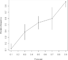
Figure 3: Reliability diagram for the forecasts $\hat{p}_{t,k}$. At the midpoint of each of the five bins $[(j-1)/5,j/5],j=1,\ldots,5$, a 95% confidence interval, centered at $\bar{Y}(j)$, for $\bar{p}(j)$ is shown; only the upper (or lower) half of the interval is shown at $j=1$ (or $5$) to keep the range of the vertical axis between $0.1$ and $0.9$.

Table 3 gives the means, standard deviations (SD), and 5-number summaries of $\bar{Y}(j),\bar{p}(j),\hat{v}(j)$ and $v(j)$ defined in (3.5), (25) and (29) based on the 1,000 simulations. In particular, it shows that $\hat{v}(j)$ tends to

Table 3: Simulation results for $\bar{p}(j),\bar{Y}(j),v(j)$ and $\hat{v}(j)$

	Min	1st qrt.	Median	3rd qrt.	Max	Mean	SD
$\bar{p}(1)$	0.101	0.101	0.101	0.168	0.234	0.121	0.033
$\bar{Y}(1)$	0.017	0.083	0.117	0.156	0.350	0.123	0.051
$v(1)$	0.087	0.087	0.087	0.127	0.167	0.100	0.020
$\hat{v}(1)$	0.067	0.089	0.106	0.132	0.233	0.106	0.037
$\bar{p}(2)$	0.101	0.300	0.300	0.355	0.515	0.320	0.049
$\bar{Y}(2)$	0.050	0.267	0.317	0.378	0.633	0.319	0.089
$v(2)$	0.087	0.207	0.207	0.207	0.247	0.209	0.015
$\hat{v}(2)$	0.048	0.208	0.221	0.239	0.259	0.213	0.034
$\bar{p}(3)$	0.300	0.515	0.515	0.577	0.701	0.527	0.058
$\bar{Y}(3)$	0.217	0.467	0.533	0.589	0.833	0.529	0.096
$v(3)$	0.206	0.233	0.247	0.247	0.247	0.239	0.011
$\hat{v}(3)$	0.144	0.240	0.249	0.254	0.259	0.244	0.015
$\bar{p}(4)$	0.515	0.659	0.701	0.701	0.906	0.690	0.052
$\bar{Y}(4)$	0.367	0.633	0.689	0.750	1.000	0.687	0.090
$v(4)$	0.082	0.206	0.206	0.206	0.247	0.204	0.021
$\hat{v}(4)$	0.063	0.207	0.217	0.236	0.259	0.211	0.035
$\bar{p}(5)$	0.769	0.906	0.906	0.906	0.906	0.895	0.026
$\bar{Y}(5)$	0.733	0.867	0.900	0.933	1.000	0.892	0.049
$v(5)$	0.082	0.082	0.082	0.082	0.164	0.088	0.016
$\hat{v}(5)$	0.077	0.084	0.093	0.120	0.202	0.096	0.037

over-estimate $v(j)$. Moreover, the probability of coverage of the 95% interval (26) for $\bar{p}(j)$, evaluated by averaging over the 1,000 simulations, is 0.949, 0.947, 0.944, 0.940 and 0.928, for $j=1,\ldots,5$, respectively, suggesting that the results of Theorem 5 still apply even for moderate sample sizes. We do not consider the second forecast $\hat{p}_{t,k}^{\prime}=\bar{Y}_{t-1}$ to illustrate reliability diagrams because by the central limit theorem, the $\hat{p}_{t,k}^{\prime}$ are concentrated around 0.5 and nearly all of the forecasts lie in the bin $[0.4,0.6]$.

5 Proofs of Theorems 4 and 5

Re-labeling the $Y_{i}$ as $Y_{t,1},\ldots,Y_{t,K_{t}}$, we note that conditional on $\mathcal{F}_{t-1},\{Y_{t,k}\dvtx 1\leq k\leq K_{t}\}$ is a set of independent Bernoulli random variables with respective parameters $p_{t,1},\ldots,p_{t,K_{t}}$. This point, which has been noted in the second paragraph of Section 3.4 and will be discussed further in Section 7, explains why we can first derive the result for the special case in which $Y_{t,k}$ are independent and then modify the argument by conditioning on $\mathcal{F}_{t-1}$ and appealing to martingale theory. As an illustration, note that if $Y_{i},i\in I_{j,t}$, are i.i.d. Bernoulli random variables with common parameter $p_{t}(j)$, then $\hat{v}_{t}(j)$ defined in (18) is an unbiased estimate of $p_{t}(j)(1-p_{t}(j))$ and one can use the classical strong law of large numbers to derive the result. The proof of Theorem 3 basically shows that $\hat{v}_{t}(j)$ is “conditionally unbiased” given $\mathcal{F}_{t-1}$ in the sense of (19) and then uses the martingale strong law to derive the result. To prove Theorem 4, we extend this idea to obtain a conditionally unbiased estimate of Var($\hat{v}_{t}(j)$) by first considering the i.i.d. case: let $X_{1},\ldots,X_{m}$ be i.i.d. random variables. As is well known, the sample variance $\hat{v}=\sum_{i=1}^{m}(X_{i}-\bar{X})^{2}/(m-1)$ is a $U$-statistic of order 2, with kernel $h(X_{i},X_{k})=(X_{i}-X_{k})^{2}/2$. Arvesen (1969) has shown that an unbiased estimate of the variance of the $U$-statistic is the jackknife estimate

$$\frac{4(m-1)}{m(m-2)^{2}}\sum_{i=1}^{m}\Biggl{\{}\frac{1}{m-1}\mathop{\sum_{k=1}}_{k\neq i}^{m}h(X_{i},X_{k})-\hat{v}\Biggr{\}}^{2}.$$ (30)

Proof of Theorem 4 Use $L(p,\hat{p})=(p-\hat{p})^{2}$ to express $n\{\hat{L}_{n}-n^{-1}\times\break\sum_{t=1}^{T}\sum_{j=1}^{J_{t}}n_{j,t}\hat{v}_{t}(j)-L_{n}\}$ as

$$\sum_{t=1}^{T}\sum_{k=1}^{K_{t}}(1-2\hat{p}_{t,k})(Y_{t,k}-p_{t,k})-\sum_{t=1}^{T}\sum_{j=1}^{J_{t}}n_{j,t}\bigl{[}\hat{v}_{t}(j)-p_{t}(j)\bigl{(}1-p_{t}(j)\bigr{)}\bigr{]},$$ (31)

which is the difference of two martingales and is therefore a martingale. To compute the conditional variance (or predictable variation) of (31), we can use the “angle bracket” notation and formulas for predictable variation and covariation [Williams (1991), Section 12.12] to obtain

$$\Biggl{\langle}\sum_{t=1}^{T}\sum_{k=1}^{K_{t}}(1-2\hat{p}_{t,k})(Y_{t,k}-p_{t,k})\Biggr{\rangle}$$

$$\qquad=\sum_{t=1}^{T}\sum_{k=1}^{K_{t}}(1-2\hat{p}_{t,k})^{2}E\bigl{(}(Y_{t,k}-p_{t,k})^{2}|\mathcal{F}_{t-1}\bigr{)}$$ (32)

$$\qquad=\sum_{t=1}^{T}\sum_{j=1}^{J_{t}}\biggl{(}\sum_{i\in I_{j,t}}(1-2\hat{p}_{i})^{2}\biggr{)}p_{t}(j)\bigl{(}1-p_{t}(j)\bigr{)},$$

$$\Biggl{\langle}\sum_{t=1}^{T}\sum_{k=1}^{K_{t}}(1-2\hat{p}_{t,k})(Y_{t,k}-p_{t,k}),\sum_{t=1}^{T}\sum_{j=1}^{J_{t}}n_{j,t}\bigl{[}\hat{v}_{t}(j)-p_{t}(j)\bigl{(}1-p_{t}(j)\bigr{)}\bigr{]}\Biggr{\rangle}$$

(33)

$$\qquad=\sum_{t=1}^{T}\sum_{j=1}^{J_{t}}\biggl{[}\sum_{i\in I_{j,t}}(1-2\hat{p}_{i})\biggr{]}p_{t}(j)\bigl{(}1-p_{t}(j)\bigr{)}\bigl{(}1-2p_{t}(j)\bigr{)},$$

$$\Biggl{\langle}\sum_{t=1}^{T}\sum_{j=1}^{J_{t}}n_{j,t}\bigl{[}\hat{v}_{t}(j)-p_{t}(j)\bigl{(}1-p_{t}(j)\bigr{)}\bigr{]}\Biggr{\rangle}$$

$$\qquad=\sum_{t=1}^{T}\sum_{j=1}^{J_{t}}\bigl{\{}n_{j,t}p_{t}(j)\bigl{(}1-p_{t}(j)\bigr{)}\bigl{[}1-4p_{t}(j)\bigl{(}1-p_{t}(j)\bigr{)}\bigr{]}$$ (34)

$$\hskip 70.5pt\qquad\quad{}+2n_{j,t}p_{t}^{2}(j)\bigl{(}1-p_{t}(j)\bigr{)}^{2}/(n_{j,t}-1)\bigr{\}}.$$

Combining (5), (5) and (5) yields formula (4) for the conditional variance of (31) divided by $n$.

In view of (19), $\hat{v}_{t}(j)$ is a conditionally unbiased estimate of $p_{t}(j)(1-p_{t}(j))$ given $\mathcal{F}_{t-1}$. If $Y\sim$ Bernoulli$(p_{i})$, then $E(Y-p)^{3}=p(1-p)(1-2p)$. Hence a conditionally unbiased estimate of $p_{t}(j)(1-p_{t}(j))(1-2p_{t}(j))$ given $\mathcal{F}_{t-1}$ is

$$[n_{j,t}^{2}/(n_{j,t}-1)^{3}]\sum_{i\in I_{j,t}}\bigl{(}Y_{i}-\bar{Y}_{t}(j)\bigr{)}^{3},$$ (35)

analogous to (19). Replacing $p_{t}(j)(1-p_{t}(j))(1-2p_{t}(j))$ in (5) by (35) and multiplying (5) by $-2/n$ gives the second summand of (4). Note that the first summand of (4) corresponds to replacing $p_{t}(j)(1-p_{t}(j))$ in (5) by $\hat{v}_{t}(j)$. The last summand of (4) corresponds to using the jackknife estimate (30) to estimate the conditional variance of $\hat{v}_{t}(j)$ given $\mathcal{F}_{t-1}$. Since $\{Y_{i},i\in I_{j,t}\}$ is a set of i.i.d. random variables conditional on $\mathcal{F}_{t-1}$, the jackknife estimate is conditionally unbiased given $\mathcal{F}_{t-1}$; see the paragraph preceding the proof of this theorem. The rest of the argument is similar to that of Theorem 3. Proof of Theorem 5 We first prove (iii). Using the notation in the paragraph preceding the proof of Theorem 4, recall that conditional on $\mathcal{F}_{t-1}$, the $Y_{t,k}$ are independent Bernoulli($p_{t,k}$) random variables. Since $I_{j,t}$ is $\mathcal{F}_{t-1}$-measurable, it follows that $\sum_{i\in I_{j,t}}(Y_{i}-p_{i})$ is a martingale difference sequence with respect to $\{\mathcal{F}_{t}\}$ and $E\{[\sum_{i\in I_{j,t}}(Y_{i}-p_{i})]^{2}|\mathcal{F}_{t-1}\}=\sum_{i\in I_{j,t}}p_{i}(1-p_{i})$. Since $n^{-1}\sum_{t=1}^{T}\sum_{i\in I_{j,t}}p_{i}(1-p_{i})$ converges in probability to a nonrandom positive constant as $n\to\infty$, we can apply the martingale central limit theorem as in the proof of Theorem 1 to conclude that

$$\frac{\sum_{t=1}^{T}\sum_{i\in I_{j,t}}(Y_{i}-p_{i})}{\{\sum_{t=1}^{T}\sum_{i\in I_{j,t}}p_{i}(1-p_{i})\}^{1/2}}\Longrightarrow N(0,1)$$

proving the first part of (iii).

To prove the second part of (iii), and also (i) and (ii), we first show that for any nonnegative $\mathcal{F}_{t-1}$-measurable random variables $w_{t,1},\ldots,w_{t,K_{t}}$,

$$E\biggl{\{}\sum_{k\in I_{j,t}}w_{t,k}\bigl{(}Y_{t,k}-\bar{Y}_{t}(j)\bigr{)}^{2}|\mathcal{F}_{t-1}\biggr{\}}$$

(36)

$$\qquad\geq\sum_{k\in I_{j,t}}(1-n_{j,t}^{-1})w_{t,k}p_{t,k}(1-p_{t,k}),$$

in which $\sum_{k\in I_{j,t}}$ means $\sum_{i\in I_{j,t}}$ when $i$ is represented as $(t,k)$; see the second paragraph of Section 3.4. Define $\bar{Y}_{t}(j),\bar{Y}(j)$ and $\bar{p}(j)$ as in (3.5) and (25), and let $\bar{p}_{t}(j)=(\sum_{k\in I_{j,t}}p_{t,k})/n_{j,t}$. From the decomposition

$$Y_{t,k}-\bar{Y}_{t}(j)=(Y_{t,k}-p_{t,k})+\bigl{(}p_{t,k}-\bar{p}_{t}(j)\bigr{)}+\bigl{(}\bar{p}_{t}(j)-\bar{Y}_{t}(j)\bigr{)},$$ (37)

it follows that the left-hand side of (5) is equal to

$$\sum_{k\in I_{j,t}}w_{t,k}E[(Y_{t,k}-p_{t,k})^{2}|\mathcal{F}_{t-1}]+\sum_{k\in I_{j,t}}w_{t,k}\bigl{(}p_{t,k}-\bar{p}_{t}(j)\bigr{)}^{2}$$

$$\qquad{}+\sum_{k\in I_{j,t}}w_{t,k}E\bigl{[}\bigl{(}\bar{Y}_{t}(j)-\bar{p}_{t}(j)\bigr{)}^{2}|\mathcal{F}_{t-1}\bigr{]}$$ (38)

$$\qquad{}-2E\biggl{[}\bigl{(}\bar{Y}_{t}(j)-\bar{p}_{t}(j)\bigr{)}\sum_{k\in I_{j,t}}w_{t,k}(Y_{t,k}-p_{t,k})\biggr{]}$$

by using the fact that conditional on $\mathcal{F}_{t-1}$ the $Y_{t,k}$ are independent Bernoulli. Since $\bar{Y}_{t}(j)-\bar{p}_{t}(j)=\sum_{k\in I_{t,j}}(Y_{t,k}-p_{t,k})/n_{j,t}$, we can use this fact again to combine the last two terms of (5) into

$$-\sum_{k\in I_{j,t}}(w_{t,k}/n_{j,t})E[(Y_{t,k}-p_{t,k})^{2}|\mathcal{F}_{t-1}].$$ (39)

Since $w_{t,k}\geq 0$, we can drop the second term in (5) to obtain (5) from (5) and (39). Moreover, since this term is actually 0 when the $p_{t,k}$ are all equal for $k\in I_{j,t}$, equality holds in (5) in this case.

Let $w_{t,k}=n_{j,t}/(n_{j,t}-1)$. Then (5) reduces to

$$E(n_{j,t}\hat{v}_{t}(j)|\mathcal{F}_{t-1})\geq\sum_{k\in I_{j,t}}p_{t,k}(1-p_{t,k}).$$ (40)

Under the assumptions of part (iii) of the theorem, we can apply the martingale strong law to obtain

$$\qquad\sum_{t=1}^{T}\{n_{j,t}\hat{v}_{t}(j)-E(n_{j,t}\hat{v}_{t}(j)|\mathcal{F}_{t-1})\}/n_{j}\longrightarrow 0\qquad\mbox{a.s. on }\{n_{j}\to\infty\}.$$ (41)

Combining (40) with (41) yields $\hat{v}(j)\geq v(j)+o_{p}(1)$, with equality when the $p_{t,k}$ are all equal for $k\in I_{j,t}$.

To prove part (i) of the theorem, put $w_{t,k}=\{L(1,\hat{p}_{t,k})-L(0,\hat{p}_{t,k})\}^{2}n_{j,t}/\break(n_{j,t}-1)$ in (5) and then use the same argument as in the preceding paragraph. The proof of part (ii) is similar.

6 Extensions and connections to forecast comparison in econometrics

Our new approach to evaluating probability forecasts in Section 3 is based on consistent and asymptotically normal estimates of the average loss$n^{-1}\sum_{i=1}^{n}L(p_{i},\hat{p}_{i})$, without any assumptions on how the observed indicator variables $Y_{i}$ and their forecasts $\hat{p}_{i}$ are generated. The key to this approach is that conditional on $\mathcal{F}_{i-1}$, $Y_{i}$ is Bernoulli$(p_{i})$, and therefore martingale arguments can be used to derive the results in Section 3. In Section 6.1 we show how this approach can be extended to more general random variables $Y_{i}$. As shown in (5), when $Y_{i}$ is an indicator variable, the conditional expectation of the score $L(Y_{i},\hat{p}_{i})$ given $\mathcal{F}_{i-1}$ is a linear function of $p_{i}$, but this does not extend to more general random variables $Y_{i}$. In Section 6.2 we review the recent econometrics literature on testing the equality of the expected scores of two forecasts and discuss an alternative approach to statistical inference on the expected difference in average scores of two forecasts.

6.1 Extensions to general predictands

A characteristic of $(\hat{p}_{i},Y_{i})$ in probability forecasting is that $E(Y_{i}|\mathcal{F}_{i-1})=p_{i}$ while the $\mathcal{G}_{i-1}$-measurable forecast $\hat{p}_{i}$ is an estimate of $p_{i}$. The theorems in Section 3 and their martingale proofs in Section 5 can be easily extended to general random variables $Y_{i}$ when the loss function is of the form $L(\mu_{i},\hat{\mu}_{i})$, where $\mu_{i}=E(Y_{i}|\mathcal{F}_{i-1})$ and $\hat{\mu}_{i}$ is a forecast of $Y_{i}$ given $\mathcal{F}_{i-1}$. Although $Y_{i}|\mathcal{F}_{i-1}\sim$ Bernoulli$(p_{i})$ in Section 3, no parametric assumptions are actually needed when we use a loss function of the form $L(\mu_{i},\hat{\mu}_{i})$. As in (4), such loss function is said to have a linear equivalent $\tilde{L}$ if

$$\qquad\tilde{L}(y,\hat{y})\mbox{ is linear in $y$}\quad\mbox{and}\quad L(y,\hat{y})-\tilde{L}(y,\hat{y})\mbox{ does not depend on }\hat{y}.$$ (42)

The bucket model in Section 3.4 can be extended so that $Y_{t,k}|\mathcal{F}_{t-1}$ have the same mean and variance for all $(t,k)$ belonging to the same bucket. In place of (18), we now use

$$\hat{v}_{t}(j)=\sum_{i\in I_{j,t}}\bigl{(}Y_{i}-\bar{Y}_{t}(j)\bigr{)}^{2}/(n_{j,t}-1)$$ (43)

as an unbiased estimate of the common conditional variance of $Y_{i}$ given $\mathcal{F}_{i-1}$ for $i=(t,k)\in I_{j,t}$, using the same notation as that in the proof of Theorem 4. While the extension of Theorem 3 only needs the first two moments of $Y_{t,k}|\mathcal{F}_{t-1}$ to be equal for all $(t,k)$ belonging to the same bucket, Theorem 4 can also be extended by assuming the first four moments of $Y_{t,k}|\mathcal{F}_{t-1}$ to be equal for all $(t,k)$ belonging to the same bucket, by using Arvesen’s (1969) jackknife estimate of the variance of a $U$-statistic.

Clearly (37), (5) and (39) also hold with $p_{t,k}$ and $\bar{p}_{t}(j)$ replaced by $\mu_{t,k}$ and $\bar{\mu}_{t}(k)$, so Theorem 5 can likewise be extended to quasi-buckets and reliability diagrams for the predicted means $\hat{\mu}_{t,k}$. For sample means in the case of independent observations within each bucket, this extension of Theorem 5 can be viewed as a corollary of the analysis of variance. In fact, the proof of Theorem 5 uses martingale arguments and conditioning to allow dependent observations in each (quasi-)bucket.

6.2 Inference on expected difference in average scores of two forecasts

When the $Y_{i}$ are indicator variables of events, Theorem 2(ii) establishes asymptotic normality for the difference $\hat{\Delta}_{n}=n^{-1}\sum_{i=1}^{n}\{L(Y_{i},\hat{p}_{i}^{\prime})-L(Y_{i},\hat{p}_{i}^{\prime\prime})\}$ in average scores between two forecasts, from which one can perform inference on

$$\Delta_{n} = n^{-1}\sum_{i=1}^{n}E\{L(Y_{i},\hat{p}_{i}^{\prime})-L(Y_{i},\hat{p}_{i}^{\prime\prime})|\mathcal{F}_{i-1}\}$$

$$= n^{-1}\sum_{i=1}^{n}\{\delta_{i}p_{i}+L(0,\hat{p}_{i}^{\prime})-L(0,\hat{p}_{i}^{\prime\prime})\},$$

where $\delta_{i}=\{L(1,\hat{p}_{i}^{\prime})-L(0,\hat{p}_{i}^{\prime})\}-\{L(1,\hat{p}_{i}^{\prime\prime})-L(0,\hat{p}_{i}^{\prime\prime})\}$. This simplicity, however, does not extend to general $Y_{i}$.

Proper scoring rules for probability forecasts of categorical and continuous variables $Y_{i}$ have been an active area of research; see the review by Gneiting and Raftery (2007). Another active area of research is related to the extension of $\hat{\Delta}_{n}$ to general $Y_{i}$ in the econometrics literature, beginning with the seminal paper of Diebold and Mariano (1995). They consider the usual forecast errors $e_{t}:=Y_{t}-\hat{Y}_{t|t-1}$ in time series analysis, where $\hat{Y}_{t|t-1}$ is the one-step ahead forecast of $Y_{t}$ based on observations up to time $t-1$. Unlike a probability forecast that gives a predictive distribution of $Y_{t}$ as in Gneiting and Raftery (2007), $\hat{Y}_{t|t-1}$ is a nonprobabilistic forecast that predicts the value of $Y_{t}$ [see Wilks (2005), Section 7.3]. The score used by Diebold and Mariano (1995) is of the form $L(Y_{t},\hat{Y}_{t|t-1})=g(e_{t})$, and they consider the average loss differential

$$\hat{\Delta}_{n}=n^{-1}\sum_{t=1}^{n}\{L(Y_{t},\hat{Y}_{t|t-1}^{\prime})-L(Y_{t},\hat{Y}_{t|t-1}^{\prime\prime})\}$$ (45)

between two forecasts $Y_{t|t-1}^{\prime}$ and $\hat{Y}_{t|t-1}^{\prime\prime},1\leq t\leq n$. Assuming a probability measure $Q$ under which $d_{t}:=g(e_{t}^{\prime})-g(e_{t}^{\prime\prime})$ is covariance stationary with absolutely summable autocovariances $\gamma_{k}$ so that $f(0):=\sum_{k=-\infty}^{\infty}\gamma_{k}/(2\pi)$ is the spectral density at frequency 0, they use the asymptotic normality of $\hat{\Delta}_{n}$ under the null hypothesis $H_{0}\dvtx E_{Q}(d_{t})=0$ and a window estimate $\hat{f}(0)$ of $f(0)$ so that the test statistic $\sqrt{n}\hat{\Delta}_{n}/(2\pi\hat{f}(0))^{1/2}$ has a limiting standard normal distribution under $H_{0}$ as $n\to\infty$. This aysmptotic normality result, however, requires additional assumptions, such as stationary mixing, which they do not mention explicitly. Their work has attracted immediate attention and spawned many subsequent developments in the econometrics literature on this topic.

Giacomini and White (2006), hereafter abbreviated as G&W, review some of the developments and propose a refinement of $H_{0}$ for which the asymptotic normality of $\hat{\Delta}_{n}$ can be established under precisely stated conditions that can also allow nonstationarity. They formulate the null hypothesis of equal predictive ability of two forecasting models or methods as “a problem of inference about conditional expectations of forecasts and forecast errors that nests the unconditional expectations that are the sole focus of the existing literature.” The econometrics literature they refer to is primarily concerned with “forecast models;” thus $Q$ in the previous paragraph is the probability measure associated with the forecast model being evaluated, or with a more general model than the two competing forecast models whose predictive abilities are compared.

G&W evaluate not only the forecasting model but also the forecasting method, which includes “the forecasting model along with a number of choices,” such as the estimation procedure and the window of past data, used to produce the forecast. They consider $k$-step ahead forecasts, for which $\hat{Y}_{t|t-1}$ is replaced by $\hat{Y}_{t|t-k}$, and assume that the forecasts are based on finite-memory models involving unknown parameters, that is,

$$\hat{Y}_{t+k|t}=h(Y_{t},\ldots,Y_{t-m+1},\mathbf{x}_{t},\ldots,\mathbf{x}_{t-m+1};{\bolds\beta}),$$ (46)

where $h$ is a known function, $m$ is the order of the model, $\mathbf{x}_{t}$ is a covariate vector at time $t$ and ${\bolds\beta}$ is a parameter vector to be estimated from some specified window of past data. Their formulation generalizes that of West (1996) who considers regression models. Whereas West assumes that the data are actually generated by the regression model with true parameter ${\bolds\beta}^{*}$, G&W allow model misspecification, and therefore their assumptions do not involve ${\bolds\beta}^{*}$. They consider two such nominal models, resulting in the forecasts $\hat{Y}_{t|t-k}^{\prime}$ and $\hat{Y}_{t|t-k}^{\prime\prime}$ that use the same covariates but different estimates $\hat{\bolds\beta}_{t}^{\prime}$ and $\hat{\bolds\beta}_{t}^{\prime\prime}$. Their null hypothesis

$$H_{0}\dvtx E\{L(Y_{t},\hat{Y}_{t|t-k}^{\prime})-L(Y_{t},\hat{Y}_{t|t-k}^{\prime\prime})|\mathcal{G}_{t-k}\}=0\qquad\mbox{a.s. }\forall t\geq 1$$ (47)

seems to be stronger than $EL(Y_{t},Y_{t|t-k}^{\prime})=EL(Y_{t},Y_{t|t-k}^{\prime\prime})$ $\forall t$ considered by Diebold and Mariano (1995) for the case $k=1$. On the other hand, (47) in the case $k=1$ just says that $L(Y_{t},Y_{t|t-1}^{\prime})-L(Y_{t},Y_{t|t-1}^{\prime\prime})$ is a martingale difference sequence under $H_{0}$ so that the martingale central limit theorem can be applied to derive the limiting $\chi^{2}$-distribution of G&W’s test statistics under $H_{0}$. Unlike Diebold and Mariano (1995) for the case $k=1$, G&W do not use test statistics of the form (45) and their test statistics involve more complicated weighted sums of $L(Y_{t},\hat{Y}_{t|t-k}^{\prime})-L(Y_{t},\hat{Y}_{t|t-k}^{\prime\prime})$. These weights are chosen to improve the power of the test and require additional mixing and moment assumptions on $(\mathbf{x}_{t},Y_{t})$ given in their Theorems 1–3.

The methodology developed in Section 3 and its extension outlined in Section 6.1 suggest an alternative approach to comparing econometric forecasts. As in (45), we consider the average score difference

$$\hat{\Delta}_{n}=n^{-1}\sum_{i=1}^{n}\{L(Y_{t},\hat{Y}_{t}^{\prime})-L(Y_{t},\hat{Y}_{t}^{\prime\prime})\},$$ (48)

in which $\hat{Y}_{t}^{\prime}$ and $\hat{Y}_{t}^{\prime\prime}$ are forecasts that are $\mathcal{G}_{t-1}$-measurable. Since $k$-step ahead forecasts of $Y_{t}$ are $\mathcal{G}_{t-1}$-measurable for any $k\geq 1$, the theory applies to all $k$-step ahead forecasts of $Y_{t}$, as illustrated in Table 1. Instead of hypothesis testing, our approach is targeted toward estimating

$$\Delta_{n}=n^{-1}\sum_{i=1}^{n}E\{L(Y_{t},\hat{Y}_{t}^{\prime})-L(Y_{t},\hat{Y}_{t}^{\prime\prime})|\mathcal{G}_{t-1}\},$$ (49)

in which $E$ is with respect to the actual but unknown probability measure $P$. Analogously to Theorem 2(i) for the case of binary $Y_{i}$, we can apply the martingale central limit theorem to establish the asymptotic normality of $\hat{\Delta}_{n}-\Delta_{n}$. In many applications, one can make use of the bucket structure of the type in Section 3.4 to estimate the asymptotic variance of $\hat{\Delta}_{n}$. In particular, this structure is inherent in dynamic panel data in econometrics and longitudinal data in epidemiology, which is beyond the scope of this paper on forecasting probabilities of events and will be treated elsewhere. Note that the bucket structure is only used in estimating the asymptotic variance of $\hat{\Delta}_{n}$ by (43), and that Theorem 5 and its extension outlined in Section 6.1 imply that the variance estimate tends to be conservative if the assumed bucket structure actually fails to hold.

7 Discussion

The average score $n^{-1}\sum_{i=1}^{n}L(Y_{i},\hat{p}_{i})$ measures the divergence of the predicted probabilities $\hat{p}_{i}$, which lie between 0 and 1, from the indicator variables $Y_{i}$ that can only have values 0 or 1. As noted by Lichtendahl and Winkler (2007), this tends to encourage more aggressive bets on the binary outcomes, rather than the forecaster’s estimates of the event probabilities. For example, an estimate of 95% probability may lead to a probability forecast of 100% for a higher reward associated with the indicator variable $Y_{i}$; see also Mason (2008), who gives an example in which a forecaster is encouraged to give such “dishonest” forecasts. This difficulty would disappear if one uses $L$ to compare $\hat{p}_{i}$ with the actual $p_{i}$, rather than with the Bernoulli($p_{i}$) random variable $Y_{i}$. Because the $p_{i}$ are unknown, this is not feasible and the importance of using a proper score $L(Y_{i},\hat{p}_{i})$ to evaluate a probability forecast has been emphasized to address the issue of dishonest forecasts. In Section 3.2 we have shown that it is possible to use $L(p_{i},\hat{p}_{i})-L(p_{i},\hat{p}_{i}^{\prime})$ for comparing two forecasters and to construct confidence intervals of the average loss difference. A key idea underlying this development is the linear equivalent of a loss function introduced in Section 2. Schervish (1989), Section 3, has used a framework of two-decision problems involving these loss functions to develop a method for comparing forecasters. Our approach that considers $L(p_{i},\hat{p}_{i}^{\prime})-L(p_{i},\hat{p}_{i}^{\prime\prime})$ can be regarded as a further step in this direction.

As noted in Section 3.5, an important assumption underlying statistical inference in the verification of probability forecasts in meteorology is that the forecast-observation pairs are independent realizations from the joint distribution of forecasts and observations. Although Mason [(2008), page 32] has pointed out that this assumption cannot hold “if the verification score is calculated using forecasts for different locations, or if both the forecasts and observations are not independent temporally,” not much has been done to address this problem other than using moving-blocks bootstrap [Mason (2008), Wilks (2005)] because traditional statistical inference does not seem to provide much help in tackling more general forecast-observation pairs. The new approach in Section 3 can be used to resolve this difficulty. It uses martingale theory to allow the forecast-observation pairs to be generated by general stochastic systems, without the need to model the underlying system in carrying out the inference. The treatment of spatial dependence is also covered in Section 3.5, in which dependence of the events at $K_{t}$ locations at time $t$ is encapsulated in the highly complex joint distribution of their generating probabilities $p_{t,1},\ldots,p_{t,K_{t}}$, which our approach does not need to model in performing inference on forecast validation. Our viewpoint in forecast evaluation is that one should try not to make unnecessary or arbitrary assumptions on the underlying data-generating mechanism, especially in regulatory settings such as regulatory supervision of a bank’s internal ratings models of loan default probabilities; see Section 3.4 and Lai and Wong (2008). A convenient but incorrect data-generating model that is assumed can unduly bias the comparison.

References

- Arvesen (1969) {barticle}[mr] \bauthor\bsnmArvesen, \bfnmJames N.\binitsJ. N. (\byear1969). \btitleJackknifing -statistics. \bjournalAnn. Math. Statist. \bvolume40 \bpages2076–2100. \bidissn=0003-4851, mr=0264805 \bptokimsref \endbibitem
- Basel Committee on Banking Supervision (2006) {bmisc}[auto:STB—2011/09/12—07:03:23] \borganizationBasel Committee on Banking Supervision (\byear2006). \bhowpublishedBasel II: International convergence of capital measurement and capital standards: A revised framework. Available at http://www.bis.org/publ/bcbs128.htm. \bptokimsref \endbibitem
- Brier (1950) {barticle}[auto:STB—2011/09/12—07:03:23] \bauthor\bsnmBrier, \bfnmG. W.\binitsG. W. (\byear1950). \btitleVerification of forecasts expressed in terms of probability. \bjournalMonthly Weather Review \bvolume78 \bpages1–3. \bptokimsref \endbibitem
- Bröcker and Smith (2007) {barticle}[auto:STB—2011/09/12—07:03:23] \bauthor\bsnmBröcker, \bfnmJ.\binitsJ. and \bauthor\bsnmSmith, \bfnmL. A.\binitsL. A. (\byear2007). \btitleIncreasing the reliability of reliability diagrams. \bjournalWeather and Forecasting \bvolume22 \bpages651–661. \bptokimsref \endbibitem
- Cox (1958) {barticle}[auto:STB—2011/09/12—07:03:23] \bauthor\bsnmCox, \bfnmD. R.\binitsD. R. (\byear1958). \btitleTwo further applications of a model for binary regression. \bjournalBiometrika \bvolume45 \bpages562–565. \bptokimsref \endbibitem
- Dawid (1982) {barticle}[mr] \bauthor\bsnmDawid, \bfnmA. P.\binitsA. P. (\byear1982). \btitleThe well-calibrated Bayesian. \bjournalJ. Amer. Statist. Assoc. \bvolume77 \bpages605–613. \bidissn=0162-1459, mr=0675887 \bptokimsref \endbibitem
- de Finetti (1975) {bbook}[auto:STB—2011/09/12—07:03:23] \bauthor\bparticlede \bsnmFinetti, \bfnmB.\binitsB. (\byear1975). \btitleTheory of Probability: A Critical Introductory Treatment. Vol. 2. \bpublisherWiley, \baddressLondon. \bnoteTranslated from the Italian by Antonio Machì and Adrian Smith. \bidmr=0440641 \bptokimsref \endbibitem
- DeGroot and Fienberg (1983) {barticle}[auto:STB—2011/09/12—07:03:23] \bauthor\bsnmDeGroot, \bfnmM. H.\binitsM. H. and \bauthor\bsnmFienberg, \bfnmS. E.\binitsS. E. (\byear1983). \btitleThe comparison and evaluation of forecasters. \bjournalStatistician \bvolume32 \bpages12–22. \bptokimsref \endbibitem
- Diebold and Mariano (1995) {barticle}[mr] \bauthor\bsnmDiebold, \bfnmFrancis X.\binitsF. X. and \bauthor\bsnmMariano, \bfnmRoberto S.\binitsR. S. (\byear1995). \btitleComparing predictive accuracy. \bjournalJ. Bus. Econom. Statist. \bvolume13 \bpages253–263. \bptnotecheck year\bptokimsref \endbibitem
- Fox and Birke (2002) {barticle}[pbm] \bauthor\bsnmFox, \bfnmCraig R.\binitsC. R. and \bauthor\bsnmBirke, \bfnmRichard\binitsR. (\byear2002). \btitleForecasting trial outcomes: Lawyers assign higher probability to possibilities that are described in greater detail. \bjournalLaw Hum. Behav. \bvolume26 \bpages159–173. \bidissn=0147-7307, pmid=11985296 \bptokimsref \endbibitem