Probabilistic wind speed forecasting in Hungary

Abstract

Prediction of various weather quantities is mostly based on deterministic numerical weather forecasting models. Multiple runs of these models with different initial conditions result ensembles of forecasts which are applied for estimating the distribution of future weather quantities. However, the ensembles are usually under-dispersive and uncalibrated, so post-processing is required.

In the present work Bayesian Model Averaging (BMA) is applied for calibrating ensembles of wind speed forecasts produced by the operational Limited Area Model Ensemble Prediction System of the Hungarian Meteorological Service (HMS).

We describe two possible BMA models for wind speed data of the HMS and show that BMA post-processing significantly improves the calibration and precision of forecasts.

Key words: Bayesian Model Averaging, gamma distribution, continuous ranked probability score.

1 Introduction

The aim of weather forecasting is to give a good prediction of the future states of the atmosphere on the basis of present observations and mathematical models describing the dynamics (physical behaviour) of the atmosphere. These models consist of sets of non-linear partial differential equations which have only numerical solutions. The problem with these numerical weather prediction models is that the solutions highly depend on the initial conditions which are always in a way or in another not fully accurate. A possible solution to address this problem is to run the model with different initial conditions and produce ensembles of forecasts. With the help of ensembles one can estimate the distribution of future weather variables which leads us to probabilistic weather forecasting (Gneiting and Raftery,, 2005). The ensemble prediction method was proposed by Leith, (1974) and since its first operational implementation (Buizza et al.,, 1993; Toth and Kalnay,, 1997) it became a widely used technique all over the world. However, despite e.g. the ensemble mean gives a better estimate of a meteorological quantity than most or all of the ensemble members, the ensemble is usually under-dispersive and in this way, uncalibrated. This phenomena was observed at several operational ensemble prediction systems, for an overview see e.g. Buizza et al., (2005).

The Bayesian model averaging (BMA) method for post-processing ensembles in order to calibrate them was introduced by Raftery et al., (2005). The basic idea of BMA is that to each ensemble member forecast corresponds a conditional probability density function (PDF) that can be interpreted as the conditional PDF of the future weather quantity provided the considered forecast is the best one. Then the BMA predictive PDF of the future weather quantity is the weighted sum of the individual PDFs corresponding to the ensemble members and the weights are based on the relative performances of the ensemble members during a given training period. In Raftery et al., (2005) the BMA method was successfully applied to obtain 48 hour forecasts of surface temperature and sea level pressure in the North American Pacific Northwest based on the 5 members of the University of Washington Mesoscale Ensemble (Grimit and Mass,, 2002). These weather quantities can be modeled by normal distributions, so the predictive PDF is a Gaussian mixture. Later Sloughter et al., (2007) developed a discrete-continuous BMA model for precipitation forecasting, where the discrete part corresponds to the event of no precipitation, while the cubic root of the precipitation amount (if it is positive) is modeled by a gamma distribution. In Sloughter et al., (2010) the BMA method was used for wind speed forecasting and the component PDFs follow gamma distribution. Finally, using von Mises distribution to model angular data Bao et al., (2010) introduced a BMA scheme to predict surface wind direction.

In the present work we apply the BMA method for calibrating ensemble forecasts of wind speed produced by the operational Limited Area Model Ensemble Prediction System (LAMEPS) of the Hungarian Meteorological Service (HMS) called ALADIN-HUNEPS (Hágel,, 2010; Horányi et al.,, 2011). ALADIN-HUNEPS covers a large part of Continental Europe with a horizontal resolution of 12 km and it is obtained by dynamical downscaling (by the ALADIN limited area model) of the global ARPEGE based PEARP system of Météo France (Horányi et al.,, 2006; Descamps et al.,, 2009). The ensemble consists of 11 members, 10 initialized from perturbed initial conditions and one control member from the unperturbed analysis. This construction implies that the ensemble contains groups of exchangeable forecasts (the ensemble members cannot be distinguished), so for post-processing one has to use the modification of BMA as suggested by Fraley et al., (2010).

2 Data

As it was mentioned in the Introduction, BMA post-processing of ensemble predictions was applied for wind speed data obtained from the HMS. The data file contains 11 member ensembles (10 forecasts started from perturbed initial conditions and one control) of 42 hour forecasts for 10 meter wind speed (given in m/s) for 10 major cities in Hungary (Miskolc, Szombathely, Győr, Budapest, Debrecen, Nyíregyháza, Nagykanizsa, Pécs, Kecskemét, Szeged) produced by the ALADIN-HUNEPS system of the HMS, together with the corresponding validating observations, for the period between October 1, 2010 and March 25, 2011. The forecasts are initialized at 18 UTC, the startup speed of the anemometers measuring the validating observations is $0.1$ m/s. The data set is fairly complete, since there are only two days (18.10.2010 and 15.02.2011) when three ensemble members are missing for all sites and one day (20.11.2010) when no forecasts are available.

Figure 1: Verification rank histogram of the 11-member ALADIN-HUNEPS ensemble. Period: October 1, 2010 – March 25, 2011.

Figure 1 shows the verification rank histogram of the raw ensemble, that is the histogram of ranks of validating observations with respect to the corresponding ensemble forecasts. This histogram is far from the desired uniform distribution, in most of the cases the ensemble members either underestimate, or overestimate the validating observations (the ensemble range contains the observed wind speed only in $61.21\%$ of the cases). Hence, the ensemble is under-dispersive and in this way it is uncalibrated.

3 The model and diagnostics

To obtain a probabilistic forecast of wind speed the modification of BMA gamma model of Sloughter et al., (2010) for ensembles with exchangeable members (Fraley et al.,, 2010) was used. The first idea is to have two exchangeable groups: one contains the control denoted by  $f_{c}$,  the other one the 10 ensemble members corresponding to the different perturbed initial conditions which are denoted by  $f_{\ell,1},\ldots,f_{\ell,10}$,  respectively.  In this way we assume that the probability density function (PDF) of the forecasted wind speed  $x$  equals:

$$p(x|f_{c},f_{\ell,1},\ldots,f_{\ell,10};b_{0},b_{1},c_{0},c_{1})= \,\omega g(x;f_{c},b_{0},b_{1},c_{0},c_{1})$$ (3.1)

$$+\frac{1-\omega}{10}\sum_{j=1}^{10}g(x;f_{\ell,j},b_{0},b_{1},c_{0},c_{1}),$$

where  $\omega\in[0,1]$,  and   $g$  is the conditional PDF corresponding to the ensemble members. As we are working with wind speed data,  $g(x;f,b_{0},b_{1},c_{0},c_{1})$  is a gamma PDF with mean  $b_{0}+b_{1}f$  and standard deviation  $c_{0}+c_{1}f$.  Here we restrict both the mean and the standard deviation parameters to constant values for all ensemble members, which reduces the number of parameters and simplifies calculations. Mean parameters  $b_{0},\ b_{1}$  are estimated with the help of linear regression, while weight  $\omega$  and standard deviation parameters  $c_{0},\ c_{1}$,  by maximum likelihood method, using training data consisting of ensemble members and verifying observations from the preceding  $n$  days (training period). In order to handle the problem that the wind speed values under 0.1 m/s are considered to be zero, the maximum likelihood (ML) method for gamma distributions suggested by Wilks, (1990) is applied, while the maximum of the likelihood function is found with the help of EM algorithm (McLachlan and Krishnan,, 1997). For more details see Sloughter et al., (2010); Fraley et al., (2010). Once the estimated parameters for a given day are available, one can use either the mean or the median of the predictive PDF (3.1) as a point forecast.

Figure 2: Plume diagram of ensemble forecast of 10 meter wind speed for Debrecen initialized at 18 UTC, 22.10.2010.

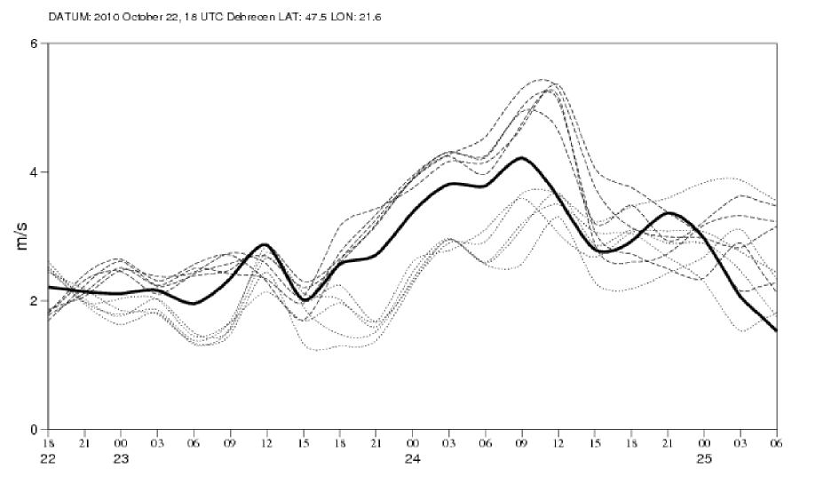
Based on a more careful look on the ensemble members there are some differences in the generation of the ten exchangeable ensemble members. To obtain them only five perturbations are calculated and then they are added to (odd numbered members) and subtracted from (even numbered members) the unperturbed initial conditions (Horányi et al.,, 2011). Figure 2 shows the plume diagram of ensemble forecast of 10 meter wind speed for Debrecen initialized at 18 UTC, 22.10.2010. (solid line: control; dotted line: odd numbered members, dashed line: even numbered members). This diagram clearly illustrates that the behaviour of ensemble member groups  $\{f_{\ell,1},\ f_{\ell,3},\ f_{\ell,5},\ f_{\ell,7},\ f_{\ell,9}\}$  and  $\{f_{\ell,2},\ f_{\ell,4},\ f_{\ell,6},\ f_{\ell,8},\ f_{\ell,10}\}$  really differ from each other. Therefore, in this way one can also consider a model with three exchangeable groups: control, odd numbered exchangeable members and even numbered exchangeable members. This idea leads to the following PDF of the forecasted wind speed  $x$:

$$q(x|f_{c},f_{\ell,1},\ldots,f_{\ell,10}; \,b_{0},b_{1},c_{0},c_{1})=\omega_{c}g(x;f_{c},b_{0},b_{1},c_{0},c_{1})$$ (3.2)

$$+\sum_{j=1}^{5}\big{(}\omega_{o}g(x;f_{\ell,2j-1},b_{0},b_{1},c_{0},c_{1})+\omega_{e}g(x;f_{\ell,2j},b_{0},b_{1},c_{0},c_{1})\big{)},$$

where for weights  $\omega_{c},\omega_{o},\omega_{e}\in[0,1]$  we have  $\omega_{c}+5\omega_{o}+5\omega_{e}=1$,  while PDF  $g$  and parameters  $b_{0},b_{1},c_{0},c_{1}$  are the same as for the model (3.1). Obviously, both the weights and the parameters can be estimated in the same way as before.

 

(a) (b)

 

(c) (d)

Figure 3: Ensemble BMA PDFs (overall: thick black line; control: red line; sum of exchangeable members on (a) and (b): light blue line; on (c) and (d): green (odd members) and blue (even members) lines), ensemble members (circles with the same colours as the corresponding PDFs), ensemble BMA median forecasts (vertical black line), verifying observations (vertical orange line) and the first and last deciles (vertical dashed lines) for wind speed in Debrecen for models (3.1): (a) 30.12.2010, (b) 17.03.2011; and (3.2): (c) 30.12.2010, (d) 17.03.2011.

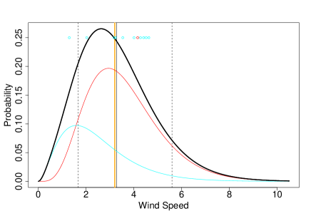
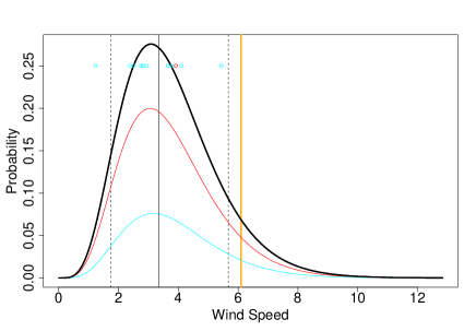
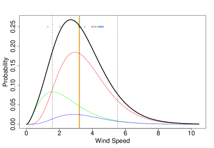
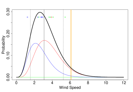
As an illustration we consider the data and forecasts for Debrecen for two different dates 30.12.2010 and 17.03.2011 for models (3.1) and (3.2). Figures 3a and 3b show the PDFs of the two groups in model (3.1), the overall PDFs, the median forecasts, the verifying observations, the first and last deciles and the ensemble members. The same functions and quantities can be seen on Figures 3c and 3d, where besides the overall PDF we have three component PDFs and three groups of ensemble members. On 30.12.2010 the spread of the ensemble members is quite fair and the ensemble range contains the validating observation (3.2 m/s). In this case the ensemble mean (3.5697 m/s) overestimates, while BMA median forecasts corresponding to the two- and three-group models (3.2876 m/s and 3.2194 m/s, respectively) are pretty close to the true wind speed. A different situation is illustrated on Figures 3b and 3d, where the spread of the ensemble is even higher, but all ensemble members underestimate the validating observation (6.1 m/s). Obviously, the same holds for the ensemble mean (3.2323 m/s) and due to the bias correction the BMA median forecasts corresponding to models (3.1) and (3.2) also give bad results (3.3409 m/s and 3.0849 m/s, respectively).

Figure 4: Average widths and coverages of $66.7\,\%$ and $90\,\%$ BMA prediction intervals corresponding to two-group model (3.1) for various training period lengths.

To check the performance of probabilistic forecasts based on models (3.1) and (3.2) and the corresponding point forecasts, as a reference we use the ensemble mean and the ensemble median. We compare the mean absolute errors (MAE) and the root mean square errors (RMSE) of these point forecasts and also the mean continuous ranked probability scores (CRPS) (Wilks,, 2006; Gneiting and Raftery,, 2007) and the coverages and average widths of $66.7\,\%$ and $90\,\%$ prediction intervals of the BMA predictive probability distributions and of the raw ensemble. We remark that for MAE and RMSE the optimal point forecasts are the median and the mean, respectively (Gneiting,, 2011; Pinson and Hagedorn,, 2011). Further, given a cumulative distribution function (CDF)  $F(y)$  and a real number  $x$,  the CRPS is defined as

$$\mathop{\hbox{\rm crps}}\big{(}F,x\big{)}:=\int_{-\infty}^{\infty}\big{(}F(y)-{\mathbbm{1}}_{\{y\geq x\}}\big{)}^{2}{\mathrm{d}}y.$$

The mean CRPS of a probability forecast is the average of the CRPS values of the predictive CDFs and corresponding validating observations taken over all locations and time points considered. For the raw ensemble the empirical CDF of the ensemble replaces the predictive CDF. The coverage of a  $(1-\alpha)100\,\%,\ \alpha\in(0,1),$  prediction interval is the proportion of validating observations located between the lower and upper  $\alpha/2$  quantiles of the predictive distribution. For a calibrated predictive PDF this value should be around  $(1-\alpha)100\,\%$.

4 Results

Figure 5: CRPS of BMA predictive distribution, MAE values of BMA median and RMSE values of BMA mean forecasts corresponding to two-group model (3.1) for various training period lengths.

Data analysis provided below was performed with the help of the ensembleBMA package of R (Fraley et al.,, 2009, 2011). As a first step the length of the appropriate training period was determined, then the performances of the BMA post-processed ensemble forecasts corresponding to models (3.1) and (3.2) were analyzed.

4.1 Training period

According to the results of e.g. Raftery et al., (2005) to determine the length of the training period to be used we compare the MAE values of BMA median forecasts, the RMSE values of BMA mean forecasts, the CRPS values of BMA predictive distributions and the coverages and average widths of $90\,\%$ and $66.7\,\%$ BMA prediction intervals for training periods of length  $10,11,\ldots,60$  calendar days. In order to ensure the comparability of the results we consider verification results from 02.12.2010 to 25.03.2011 (114 days).

Figure 6: Average widths and coverages of $66.7\,\%$ and $90\,\%$ BMA prediction intervals corresponding to three-group model (3.2) for various training period lengths.

Consider first the two-group model (3.1). On Figure 4 the average widths and coverages of $66.7\,\%$ and $90\,\%$ BMA prediction intervals are plotted against the length of the training period. The average widths of the prediction intervals show an increasing trend, so shorter training periods yield sharper forecasts. Coverages of $66.7\,\%$ and $90\,\%$ prediction intervals are not monotonously increasing, too. For short training periods the coverage of the $66.7\,\%$ prediction interval oscillates around the correct $66.7\,\%$, but for training periods not shorter than 17 days it stays above this level. The coverage of the $90\,\%$ prediction interval stabilizes above the correct $90\,\%$ for training periods longer than 24 days. Hence, to have calibrated forecasts, one should choose a training period not shorter than 25 days.

Figure 7: CRPS of BMA predictive distribution, MAE values of BMA median and RMSE values of BMA mean forecasts corresponding to three-group model (3.2) for various training period lengths.

Figure 5 shows CRPS values of BMA predictive distribution, MAE values of BMA median forecasts and RMSE values of BMA mean forecasts as functions of the training period length. CRPS and RMSE both take their minima at 28 days, the corresponding values are $0.7388$ and $1.3675$, respectively. MAE takes its minimum of $1.0472$ at 30 days, while the second smallest value ($1.0476$) is obtained with a training period of length 28 days. This means that for model (3.1) a 28 days training period seems to be reasonable and training periods longer than 30 days cannot be taken into consideration.

Similar conclusions can be drawn from Figures 6 and 7 for the three-group model (3.2). In this case the $66.7\,\%$ and $90\,\%$ prediction intervals are slightly narrower than the corresponding intervals of model (3.1), their coverages stabilize above the correct $66.7\,\%$ and $90\,\%$ for training periods longer than 17 and 24 days, respectively. CRPS and MAE plotted on Figure 7 both reach their minima of $0.7372$ and $1.0452$, respectively, at 30 days, while values $0.7376$ and $1.0456$ corresponding to training period of length 28 days are both the fourth smallest ones. RMSE takes its minimum of $1.3632$ at 27 days, and increases afterwards. The fourth smallest value ($1.3644$) again corresponds to 28 days, while the RMSE corresponding to 30 days is significantly larger ($1.3664$). Moreover, $66.7\,\%$ and $90\,\%$ prediction intervals corresponding to 28 days are sharper than the appropriate prediction intervals calculated using training period of length 30 days ($2.5813$ and $4.4340$ vs. $2.5831$ and $4.4378$). Hence, we suggest the use of a training period of length 28 days for both BMA models.

4.2 Predictions using BMA post-processing

According to the results of the previous subsection, to test the performance of BMA post-processing on the 11 member ALADIN-HUNEPS ensemble we use a training period of 28 calendar days. In this way ensemble members, validating observations and BMA models are available for 146 calendar days (on 20.11.2010 all ensemble members are missing).

Figure 8: PIT histograms for BMA post-processed forecasts using two-group (3.1) and three-group (3.2) models.

First we check the calibration of BMA post-processed forecasts with the help of probability integral transform (PIT) histograms. The PIT is the value of the BMA predictive cumulative distribution evaluated at the verifying observations (Fraley et al.,, 2010). The closer the histogram to the uniform distribution, the better is the calibration. On Figure 8 the PIT histograms corresponding to two- and three-group BMA models (3.1) and (3.2) are displayed. Compared to the verification rank histogram of the raw ensemble (see Figure 1) one can observe a large improvement with the use of calibration. However, these PIT histograms are still not perfect, e.g. Kolmogorov-Smirnov test rejects uniformity both for the two- and for the three-group model. The corresponding $p$-values are $0.0222$ and $0.0187$, respectively, so the PIT of the two-group model is slightly better.

	Coverage ($\%$)		Average Width
Interval	$66.7\,\%$ interval	$90.0\,\%$ interval	$66.7\,\%$ interval	$90.0\,\%$ interval
Raw ensemble	$38.70$	$55.14$	$1.4388$	$2.2001$
BMA model (3.1)	$68.08$	$90.34$	$2.6359$	$4.5297$
BMA model (3.2)	$68.36$	$90.21$	$2.6153$	$4.4931$

Table 1: Coverage and average width of prediction intervals.

Table 1 gives the coverages and average widths of $66.7\,\%$ and $90.0\,\%$ prediction intervals calculated using models (3.1) and (3.2), and the corresponding measures calculated from the raw ensembles. In the latter case the ensemble of forecasts corresponding to a given location and time is considered as a statistical sample. The BMA prediction intervals calculated from both models are approximately twice as wide, as the corresponding intervals of the raw ensemble. This comes from the small dispersion of the raw ensemble, see the verification rank histogram of Figure 1. Concerning calibration one can observe that the coverages of both BMA prediction intervals are rather close to the right coverages, while the coverages of the prediction intervals calculated from the raw ensemble are quite poor. This also shows that BMA post-processing highly improves calibration. Further, BMA model (3.2) yields slightly sharper predictions but there is no big difference between the coverages of the two BMA models.

	Mean CRPS	MAE		RMSE
		median	mean	median	mean
Raw ensemble	$0.8599$	$1.1215$	$1.1090$	$1.4634$	$1.4440$
BMA model (3.1)	$0.7577$	$1.0678$	$1.0763$	$1.4213$	$1.4067$
BMA model (3.2)	$0.7556$	$1.0643$	$1.0749$	$1.4153$	$1.4018$

Table 2: Mean CRPS of probabilistic, MAE and RMSE of deterministic forecasts.

Figure 9: BMA weights of two-group (3.1) and three-group (3.2) models.

On Table 2 the verification results of the model fit are given. Verification measures of probabilistic forecasts and point forecasts calculated using BMA models (3.1) and (3.2) are compared to the corresponding measures calculated for the raw ensemble. Examining these results one can clearly observe the advantage of BMA post-processing which resulted a significant decrease in all verification scores. Further, the BMA median forecasts yield slightly lower MAE values than the BMA mean forecasts for both models, while in the case of RMSE values the situation is just the opposite, which is a perfect illustration of the theoretical results of Gneiting, (2011) about the optimality of these verification scores. Finally, model (3.2) distinguishing three exchangeable groups of ensemble forecasts slightly outperforms model (3.1).

Figure 9 shows the BMA weights corresponding to models (3.1) and (3.2). Examining the behaviour of weight  $\omega$  of the control member of the ensemble in the two-group model (3.1), one can observe that in $84.56\,\%$ of the cases there is a real mixture of gamma distributions. The values of  $\omega$  which are close to $1$ correspond to a continuous time interval 17.11.2010 – 09.12.2010, when the control member of the ensemble gives much better forecasts than the ten exchangeable ensemble members. This can clearly be seen from Table 3 where the MAE and RMSE values of the particular ensemble members are given for the above mentioned period. In all of these 23 subsequent days  $\omega>0.995$  but on 20.11.2010, when  $\omega=0.9873$.  However, as it was mentioned earlier, on this particular day all ensemble forecasts are missing from the data set. The situation is quite different in the case of the three-group model (3.2), where the weight  $\omega_{c}$  of the control is close to $1$ (greater than $0.98$) only on 7 days, so in the remaining cases ($95.30\,\%$) a real mixture of gamma distributions present. Further, observe that there are 55 days  ($36.91\,\%$)  when all BMA weights are positive, the even numbered exchangeable members have nearly zero weights  (less than $0.001$)  in 45 cases  ($30.20\,\%$)  at the beginning of the considered time period, while the odd numbered exchangeable members are almost zero in 53 cases  ($35.57\,\%$),  mainly at the end of it.

	Control	Exchangeable members
	$f_{c}$	$f_{\ell,1}$	$f_{\ell,2}$	$f_{\ell,3}$	$f_{\ell,4}$	$f_{\ell,5}$	$f_{\ell,6}$	$f_{\ell,7}$	$f_{\ell,8}$	$f_{\ell,9}$	$f_{\ell,10}$
MAE	$1.32$	$1.60$	$1.46$	$1.52$	$1.68$	$1.51$	$1.49$	$1.56$	$1.42$	$1.41$	$1.65$
RMSE	$1.69$	$2.16$	$1.86$	$1.96$	$2.26$	$1.92$	$1.95$	$2.05$	$1.89$	$1.81$	$2.23$

Table 3: MAE and RMSE of the control and exchangeable ensemble forecasts for the period 17.11.2010 – 09.12.2010.

Figure 10: Parameters of two-group model (3.1) and differences in standard deviation parameters between three- and two-group models.

Finally, on Figure 10 common bias parameters  $b_{0},\ b_{1}$  of both BMA models investigated and standard deviation parameters  $c_{0},\ c_{1}$  of the two-group model (3.1) are plotted, together with the differences in standard deviation parameters of three- and two-group models. Bias parameters are rather stable, the relative standard deviations of  $b_{0}$  and  $b_{1}$  are $25.44\,\%$ and $9.97\,\%$, respectively. Hence, the BMA mean forecast of a particular day is mainly determined by the corresponding ensemble forecasts. The standard deviation parameters show more variability, for  $c_{0}$  and  $c_{1}$  the relative standard deviations are equal to $23.41\,\%$ and $41.27\,\%$ for model (3.1), and $22.64\,\%$ and $36.73\,\%$ for model (3.2).

5 Conclusions

In the present study the BMA ensemble post-processing method is applied for the 11 member ALADIN-HUNEPS ensemble of the HMS to obtain 42 hour predictions for 10 meter wind speed. Two different BMA models are investigated, one assumes two groups of exchangeable members (control and forecasts from perturbed initial conditions), while the other considers three (control and forecasts from perturbed initial conditions with positive and negative perturbations). For both models a 28 days training period is suggested. The comparison of the raw ensemble and of the probabilistic forecasts shows that the mean CRPS values of BMA post-processed forecasts are considerably lower than the mean CRPS of the raw ensemble. Further, the MAE and RMSE values of BMA point forecasts (median and mean) are also lower than the MAEs and RMSEs of the ensemble median and of the ensemble mean. The calibrations of BMA forecasts are nearly perfect, the coverages of $66.7\,\%$ and $90.0\,\%$ prediction intervals are very close to the right values. The three-group BMA model slightly outperforms the two-group one and in almost all cases yields a real mixture of gamma distributions.

In this way one can conclude that BMA post-processing of ensemble forecasts of wind speed data of the HMS significantly improves the precision and calibration of the forecasts, its operational application is worth considering.

Acknowledgments.    Research was supported by the Hungarian Scientific Research Fund under Grants No. OTKA T079128/2009 and OTKA NK101680 and by the TÁMOP-4.2.2.C-11/1/KONV-2012-0001 project. The project has been supported by the European Union, co-financed by the European Social Fund. The authors are indebted to Tilmann Gneiting for his useful suggestions and remarks and to Máté Mile and Mihály Szűcs from the HMS for providing the data.

References

- Bao et al., (2010) Bao, L., Gneiting, T., Raftery, A. E., Grimit, E. P. and Guttorp, P. (2010) Bias correction and Bayesian model averaging for ensemble forecasts of surface wind direction. Mon. Wea. Rev. 138, 1811–1821.
- Buizza et al., (1993) Buizza, R., Tribbia, J., Molteni, F. and Palmer, T. (1993) Computation of optimal unstable structures for a numerical weather prediction system. Tellus A 45, 388–407.
- Buizza et al., (2005) Buizza, R., Houtekamer, P. L., Toth, Z., Pellerin, G., Wei, M. and Zhu, Y. (2005) A comparison of the ECMWF, MSC, and NCEP global ensemble prediction systems. Mon. Wea. Rev. 133, 1076–1097.
- Descamps et al., (2009) Descamps, L., Labadier, C., Joly, A. and Nicolau, J. (2009) Ensemble Prediction at Météo France (poster introduction by Olivier Riviere) 31st EWGLAM and 16th SRNWP meetings, 28th September – 1st October, 2009. Available at: http://srnwp.met.hu/Annual_Meetings/2009/download/sept29/morning/posterpearp.pdf
- Fraley et al., (2009) Fraley, C., Raftery, A. E., Gneiting, T. and Sloughter, J. M. (2009) EnsembleBMA: An R package for probabilistic forecasting using ensembles and Bayesian model averaging. Technical Report 516R, Department of Statistics, University of Washington.
- Fraley et al., (2010) Fraley, C., Raftery, A. E. and Gneiting, T. (2010) Calibrating multimodel forecast ensembles with exchangeable and missing members using Bayesian model averaging. Mon. Wea. Rev. 138, 190–202.
- Fraley et al., (2011) Fraley, C., Raftery, A. E., Gneiting, T., Sloughter, J. M. and Berrocal, V. J. (2011) Probabilistic weather forecasting in R. The R Journal 3, 55–63.
- Gneiting and Raftery, (2005) Gneiting, T. and Raftery, A. E. (2005) Weather forecasting with ensemble methods. Science 310, 248–249.
- Gneiting and Raftery, (2007) Gneiting, T. and Raftery, A. E. (2007) Strictly proper scoring rules, prediction and estimation. J. Amer. Statist. Assoc. 102, 359–378.
- Gneiting, (2011) Gneiting, T. (2011) Making and evaluating point forecasts. J. Amer. Statist. Assoc. 106, 746–762.
- Grimit and Mass, (2002) Grimit, E. P. and Mass, C. F. (2002) Initial results of a mesoscale short-range ensemble forecasting system over the Pacific Northwest. Wea. Forecasting 17, 192–205.
- Hágel, (2010) Hágel, E. (2010) The quasi-operational LAMEPS system of the Hungarian Meteorological Service. Időjárás 114, 121–133.
- Horányi et al., (2006) Horányi, A, Kertész, S., Kullmann, L. and Radnóti, G. (2006) The ARPEGE/ALADIN mesoscale numerical modeling system and its application at the Hungarian Meteorological Service. Időjárás 110, 203–227.
- Horányi et al., (2011) Horányi, A., Mile, M., Szűcs, M. (2011) Latest developments around the ALADIN operational short-range ensemble prediction system in Hungary. Tellus A 63, 642–651.
- Leith, (1974) Leith, C. E. (1974) Theoretical skill of Monte-Carlo forecasts. Mon. Wea. Rev. 102, 409–418.
- McLachlan and Krishnan, (1997) McLachlan, G. J. and Krishnan, T. (1997) The EM Algorithm and Extensions. Wiley, New York.
- Pinson and Hagedorn, (2011) Pinson, P. and Hagedorn, R. (2011) Verification of the ECMWF ensemble forecasts of wind speed against analyses and observations. Meteorol. Appl. DOI: 10.1002/met.283.
- Raftery et al., (2005) Raftery, A. E., Gneiting, T., Balabdaoui, F. and Polakowski, M. (2005) Using Bayesian model averaging to calibrate forecast ensembles. Mon. Wea. Rev. 133, 1155–1174.
- Sloughter et al., (2010) Sloughter, J. M., Gneiting, T. and Raftery, A. E. (2010) Probabilistic wind speed forecasting using ensembles and Bayesian model averaging. J. Amer. Stat. Assoc. 105, 25–37.
- Sloughter et al., (2007) Sloughter, J. M., Raftery, A. E., Gneiting, T. and Fraley, C. (2007) Probabilistic quantitative precipitation forecasting using Bayesian model averaging. Mon. Wea. Rev. 135, 3209–3220.
- Toth and Kalnay, (1997) Toth, Z. and Kalnay, E. (1997) Ensemble forecasting at NCEP and the breeding method. Mon. Wea. Rev. 125, 3297–3319.
- Wilks, (1990) Wilks, D. S. (1990) Maximum likelihood estimation for gamma distribution using data containing zeros. J. Climate 3, 1495–1501.
- Wilks, (2006) Wilks, D. S. (2006) Statistical Methods in the Atmospheric Sciences. 2nd ed., Academic Press, New York.