Generalized Boundaries from Multiple Image Interpretations

Abstract

Boundary detection is essential for a variety of computer vision tasks such as segmentation and recognition. In this paper we propose a unified formulation and a novel algorithm that are applicable to the detection of different types of boundaries, such as intensity edges, occlusion boundaries or object category specific boundaries. Our formulation leads to a simple method with state-of-the-art performance and significantly lower computational cost than existing methods. We evaluate our algorithm on different types of boundaries, from low-level boundaries extracted in natural images, to occlusion boundaries obtained using motion cues and RGB-D cameras, to boundaries from soft-segmentation. We also propose a novel method for figure/ground soft-segmentation that can be used in conjunction with our boundary detection method and improve its accuracy at almost no extra computational cost.

1 Introduction

Boundary detection is a fundamental problem in computer vision and has been studied since the early days of the field. The majority of papers on boundary detection have focused on using only low-level cues, such as pixel intensity or color [18, 16, 14, 3, 19]. Recent work has started exploring the problem of boundary detection using higher-level representations of the image, such as motion, surface and depth cues [22, 24, 9], segmentation [1], as well as category specific information [13, 8].

Figure 1: Detection of occlusion and motion boundaries using the proposed generalized boundary detection method (Gb). First two rows: the input layers consist of color (C), soft-segmentation (S) [the first three dimensions are shown as RGB], and optical flow (OF). Last two rows: input layers are color (C), depth (D) and optical flow (OF). The same implementation is used for both; combining multiple input layers using Gb improves boundary detection. Best viewed in color.

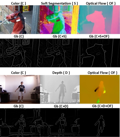
In this paper we propose a general formulation for boundary detection that can be applied, in principle, to the identification of any type of boundaries, such as general boundaries from low-level static cues, motion boundaries or category-specific boundaries (Figures 1, 6, 7). Our method can be seen both as a generalization of the early view of boundaries as step edges [11], and as a unique closed-form solution to current boundary detection problems, based on a straightforward mathematical formulation.

We generalize the classical view of boundaries from sudden signal changes on the original low-level image input [18, 16, 14, 3, 10, 6, 5], to a locally linear (planar or step-wise) model on multiple layers of the input. The layers are interpretations of the image at different levels of visual processing, which could be high-level (e.g., object category segmentation) or low-level (e.g., color or grey level intensity).

Despite the abundance of research on boundary detection, there is no general formulation of this problem. In this paper, we make the popular but implicit intuition of boundaries explicit: boundary pixels mark the transition from one relatively constant region to another, in appropriate interpretations of the image. Thus, while the region constancy assumption may only apply weakly for low-level input such as pixel intensity, it will also be weakly observed in higher-level interpretation layers of the image. Generalized boundary detection aims to exploit such weak signals across multiple layers in a principled manner. We could say that boundaries do not exist in the raw image, but rather in the multiple interpretation layers of that image. We can summarize our assumptions as follows:

1. A boundary separates different image regions, which in the absence of noise are almost constant, at some level of image interpretation or processing. For example, at the lowest level, a region could have a constant intensity. At a higher-level, it could be a region delimitating an object category, in which case the output of a category-specific classifier would be constant.

2. For a given image, boundaries in one layer often coincide, in terms of position and orientation, with boundaries in other layers. For example, discontinuities in intensity are typically correlated with discontinuities in optical flow, texture or other cues. Moreover, the boundaries that align across multiple layers often correspond to the semantic boundaries that are primarily of interest to humans: the so-called “ground-truth boundaries”.

Based on these observations, we develop a unified model, which can simultaneously consider both low-level and higher-level information.

Classical vector-valued techniques on multi-images [6, 10, 11] can be simultaneously applied to several image channels, but differ from the proposed approach in a fundamental way: they are specifically designed for low-level input, by using first or second-order derivatives of the image channels, with edge models limited to very small neighborhoods of only a few pixels (for approximating the derivatives). We argue that in order to correctly incorporate higher-level information, one must go beyond a few pixels, to much larger neighborhoods, in line with more recent methods [1, 15, 17, 19]. First, even though boundaries from one layer coincide with edges from a different layer, they cannot be required to match perfectly in location. Second, boundaries, especially in higher-level layers, do not have to correspond to sudden changes. They could be smooth transitions over larger regions and exhibit significant noise that would corrupt any local gradient computation. That is why we advocate a linear boundary model rather than one based on noisy estimation of derivatives, as discussed in the next section.

Another drawback of traditional multi-image techniques is the issue of channel scaling, where the algorithms require considerable manual tuning. Consistent with current machine learning based approaches [15, 1, 7], the parameters in our proposed method are automatically learned using real-world datasets. However, our method has better computational complexity and employs far fewer parameters. This allows us to learn efficiently from limited quantities of data without overfitting.

Another important advantage of our approach over current methods is in the closed-form computation of the boundary orientation. The idea behind $Pb$ [15] is to classify each possible boundary pixel based on the histogram difference in color and texture information between the two half disks on either side of a potential orientation, for a fixed number of candidate angles (e.g., 8). The separate computation for each orientation significantly increases the computational cost and limits orientation estimates to a particular granularity.

We summarize our contributions as follows: 1) we present a closed-form formulation of generalized boundary detection that is computationally efficient; 2) we recover exact boundary normals through direct estimation rather than evaluating coarsely sampled orientation candidates; 3) as opposed to current approaches [1, 24], our unified framework treats both low-level pixel data and higher-level interpretations equally and can easily incorporate outputs from new image interpretation algorithms; and 4) our method requires learning only a single parameter per layer, which enables efficient training with limited data. We demonstrate the strength of our method on a variety of real-world tasks.

2 Problem Formulation

For a given $N_{x}\times N_{y}$ image $I$, let the $k$-th layer $L_{k}$ be some real-valued array, of the same size, associated with $I$, whose boundaries are relevant to our task. For example, $L_{k}$ could contain, at each pixel, the real-valued output of a patch-based binary classifier trained to detect man-made structures or respond to a particular texture or color distribution. Thus, $L_{k}$ will consist of relatively constant regions (modulo classifier error) separated by boundaries. Note that the raw pixels in the corresponding regions of the original image may not be constant.

Unlike some previous approaches, we expect that boundaries in different layers may not precisely align. Given a set of layers, each corresponding to a particular interpretation level of the image, we wish to identify the most consistent boundaries across multiple layers. The output of our method for each point $\mathbf{p}$ on the $N_{x}\times N_{y}$ image grid is a real-valued probability that $\mathbf{p}$ lies on a boundary, given the information in all multiple image interpretations $L_{k}$ centered at $\mathbf{p}$.

We model a boundary point in layer $L_{k}$ as a transition (either sudden or gradual) in the corresponding values of $L_{k}$ along the normal to the boundary. If several $K$ such layers are available, let $\mathbf{L}$ be a three-dimensional array of size $N_{x}\times N_{y}\times K$, such that $L(x,y,k)=L_{k}(x,y)$, for each $k$. Thus, $\mathbf{L}$ contains all the relevant information for the current boundary detection problem, given multiple interpretations of the image or video. Figure 1 illustrates how we improve the accuracy of boundary detection by combining different useful layers of information, such as color, soft-segmentation and optical flow, in a single representation $\mathbf{L}$,

Let $\mathbf{p}_{0}$ be the center of a window $W(\mathbf{p}_{0})$ of size $\sqrt{N_{W}}\times\sqrt{N_{W}}$. For each image-location $\mathbf{p}_{0}$ we want to evaluate the probability of boundary using the information from $\mathbf{L}$, limited to that particular window. For any $\mathbf{p}$ within the window, we make the following approximation, which gives our locally linear boundary model:

$$L_{k}(\mathbf{p})\approx C_{k}(\mathbf{p_{0}})+b_{k}(\mathbf{p_{0}})\mathbf{(\hat{p}_{\epsilon}-p_{0})}^{T}\mathbf{n(p_{0})}.$$ (1)

Here $b_{k}$ is nonnegative and corresponds to the boundary “height” for layer $k$ at location $\mathbf{p_{0}}$; $\mathbf{\hat{p}_{\epsilon}}$ is the closest point to $\mathbf{p}$ (projection of $\mathbf{p}$) on the disk of radius $\epsilon$ centered at $\mathbf{p_{0}}$; $\mathbf{n(p_{0})}$ is the normal to the boundary and $C_{k}(\mathbf{p_{0}})$ is a constant over the window $W(\mathbf{p}_{0})$. This constant is useful for constructing our model (see Figure 2), but its value is unimportant, since it cancels out, as shown below. Note that if we set $C_{k}(\mathbf{p_{0}})=L_{k}(\mathbf{p_{0}})$ and use a sufficiently large $\epsilon$ such that $\mathbf{\hat{p}_{\epsilon}=p}$, our model reduces to the first-order Taylor expansion of $L_{k}(\mathbf{p})$ around the current $\mathbf{p_{0}}$.

Figure 2: Simplified $1$-dimensional view of our generalized boundary model. $\epsilon$ controls the region where the model is linear. For points outside that region the layer is assumed to be roughly constant.

Figure 3: Our boundary model for different values of $\epsilon$ relative to the window size $W$: a) $\epsilon>W$; b) $\epsilon=W/2$ ; c) $\epsilon=W/1000$. When $\epsilon$ approaches zero the boundary model becomes a step (along the normal direction passing through the window center).

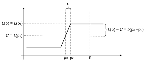
As shown in Figures 2 and 3, $\epsilon$ controls the steepness of the boundary, going from completely planar when $\epsilon$ is large (first-order Taylor expansion) to a sharp step-wise discontinuity through the window center $\mathbf{p_{0}}$, as $\epsilon$ approaches zero. More precisely, when $\epsilon$ is very small we have a step along the normal through the window center, and a sigmoid which flattens as we get farther from the center, along the boundary normal. As $\epsilon$ increases, the model flattens to become a perfect plane for any $\epsilon$ that is larger than the window radius.

When the window is far from any boundary, the value of $b_{k}$ will be near zero, since the only variation in the layer values is due to noise. If we are close to a boundary, then $b_{k}$ will become positive and large. The term $\mathbf{(\hat{p}_{\epsilon}-p_{0})}^{T}\mathbf{n(p_{0})}$ approximates the sign which indicates the side of the boundary: it does not matter on which side we are, as long as a sign change occurs when the boundary is crossed.

When a true boundary is present within several layers at the same position — i.e., $b_{k}(\mathbf{p_{0}})$ is non-zero and possibly different, for several $k$ — the normal to the boundary should be consistent. Thus, we model the boundary normal $\mathbf{n}$ as common across all layers.

We can now write the above equation in matrix form for all layers, with the same window size and location as follows. Let $\mathbf{X}$ be a $N_{W}\times K$ matrix with a row $i$ for each location $\mathbf{p_{i}}$ of the window and a column for each layer $k$, such that $X_{i;k}=L_{k}(\mathbf{p}_{i})$. Similarly, we define $N_{W}\times 2$ position matrix $\mathbf{P}$: on its $i$-th row we store the $x$ and $y$ components of $\mathbf{(\hat{p}_{\epsilon}-p_{0})}$ for the $i$-th point of the window. Let $\mathbf{n}=[n_{x},n_{y}]$ denote the boundary normal and $\mathbf{b}=[b_{1},b_{2},\ldots,b_{K}]$ the step sizes for layers $1,2,\ldots,K$. Also, let us define the rank-$1$ $2\times K$ matrix $\mathbf{J=n}^{T}\mathbf{b}$. We also define matrix $\mathbf{C}$ of the same size as $\mathbf{X}$, with each column $k$ constant and equal to $C_{k}(\mathbf{p_{0}})$.

We can then rewrite Equation 1 as follows (dropping the dependency on $\mathbf{p_{0}}$ for notational simplicity), with unknowns $\mathbf{J}$ and $\mathbf{C}$:

$$\mathbf{X\approx C+PJ}.$$ (2)

Since $\mathbf{C}$ is a matrix with constant columns, and each column of $\mathbf{P}$ sums to $0$, we have $\mathbf{P}^{T}\mathbf{C}=\mathbf{0}$. Thus, by multiplying both sides of the equation above by $\mathbf{P}^{T}$ we can eliminate the unknown $\mathbf{C}$. Moreover, it can be easily shown that $\mathbf{P}^{T}\mathbf{P}=\alpha\mathbf{I}$, i.e., the identity matrix scaled by a factor $\alpha$, which can be computed since $\mathbf{P}$ is known. We finally obtain a simple expression for the unknown $\mathbf{J}$ (since both $\mathbf{P}$ and $\mathbf{X}$ are known):

$$\mathbf{J}\approx\frac{1}{\alpha}\mathbf{P}^{T}\mathbf{X}.$$ (3)

Since $\mathbf{J=n}^{T}\mathbf{b}$ it follows that $\mathbf{JJ}^{T}=\mathbf{\|b\|^{2}n}^{T}\mathbf{n}$ is symmetric and has rank $1$. Then $\mathbf{n}$ can be estimated as the principal eigenvector of $\mathbf{M=JJ}^{T}$ and $\|\mathbf{b}\|^{2}$ as its largest eigenvalue. $\|\mathbf{b}\|$, which is obtained as the square root of the largest eigenvalue of $\mathbf{M}$, is the norm of the boundary steps vector $\mathbf{b}=[b_{1},b_{2},...,b_{K}]$. This norm captures the overall strength of boundaries from all layers simultaneously. If layers are properly scaled, then $\|\mathbf{b}\|$ could be used as a measure of boundary strength. Besides the intuitive meaning of $\|\mathbf{b}\|$, the spectral approach to boundary estimation is also related to the gradient of multi-images previously used for low-level color edge detection from classical papers such as [10, 6]. However, it is important to notice that unlike those methods, we do not compute derivatives, as they are not appropriate for higher-level layers and can be noisy for low-level layers. Instead, we fit a model, which, by controlling $\epsilon$, can vary from planar to sigmoid/step-wise. For smoother-looking results, in practice we weigh the rows of matrices $\mathbf{X}$ and $\mathbf{P}$ by a 2D Gaussian with the mean set to the window center $\mathbf{p_{0}}$ and the standard deviation equal to half of the window radius.

Once we identify $\|\mathbf{b}\|$, we pass it through a one-dimensional logistic model to obtain the probability of boundary, similarly to recent classification approaches to boundary detection [15, 1]. The parameters of the logistic regression model are learned using standard procedures. The normal to the boundary $\mathbf{n}$ is then used for non-maxima suppression.

3 Algorithm and Numerical Considerations

Before applying the main algorithm we scale each layer in $\mathbf{L}$ according to its importance, which may be problem dependent. For example, in Figure 1, it is clear that when recovering occlusion boundaries, the optical flow layer (OF) should contribute more than the raw color (C) and color-based soft segmentation (S) layers. The images displayed are from the dataset of Stein and Hebert [22]. The optical flow shown is an average between the flow [23] computed over two pairs of images: (reference frame, first frame), and (reference frame, last frame). We learn the correct scaling of the layers from training data using a standard unconstrained nonlinear optimization procedure (e.g., fminsearch routine in MATLAB) on the average $F$-measure of the training set. We apply the same learning procedure in all of our experiments. This is computationally feasible since there is only one parameter per layer in the proposed model.

Algorithm 1 Gb1: Fast Generalized Boundary Detection

  Initialize $\mathbf{L}$, scaled appropriately.

  Initialize $w_{0}$ and $w_{1}$.

  for all pixels $\mathbf{p}$ do

     $\mathbf{M\leftarrow(P}^{T}\mathbf{X_{p})(P}^{T}\mathbf{X_{p})}^{T}$

     $(\mathbf{v},\lambda)\leftarrow$ principal eigenpair of $\mathbf{M}$

     $b_{\mathbf{p}}\leftarrow\frac{1}{1+\exp(w_{0}+w_{1}\sqrt{\lambda})}$

     $\theta_{\mathbf{p}}\leftarrow\text{atan2}(v_{y},v_{x})$

  end for

  return  $\mathbf{b}$, $\mathbf{\theta}$

Algorithm 1 (referred to as Gb1) summarizes the proposed approach. The overall complexity of our method is relatively straightforward to compute. For each pixel $\mathbf{p}$, the most expensive step is the computation of the matrix $\mathbf{M}$, which takes $O((N_{W}+2)K)$ steps ($N_{W}$ is the number of pixels in the window, and $K$ is the number of layers). Since $\mathbf{M}$ is always $2\times 2$, computing its eigenpair $(\mathbf{v},\lambda)$ is a closed-form operation, with a small fixed cost. It follows that for a fixed window size $N_{W}$ and a total of $N$ pixels per image the overall complexity of our algorithm is $O(KN_{W}N)$. If $N_{W}$ is a constant fraction $f$ of $N$, then complexity becomes $O(fKN^{2})$.

Thus, the running time of Gb1 compares very favorably to that of the $Pb$ algorithm [15, 1], which in its exact form has complexity $O(fKN_{o}N^{2})$, where $N_{o}$ is a discrete number of candidate orientations. An approximation is proposed in [1] with $O(fKN_{o}N_{b}N)$ complexity where $N_{b}$ is the number of histogram bins for the different image channels. However, $N_{o}N_{b}$ is large in practice and significantly affects the overall running time.

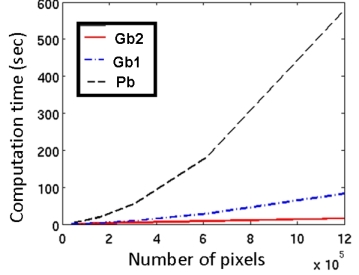
We also propose a faster version of our algorithm, Gb2, with complexity $O(fKN)$, that is linear in the number of image pixels. The speed-up is achieved by computing $\mathbf{M}$ at a constant cost (independent of the number of pixels in the window). When $\epsilon$ is large and no Gaussian weighing is applied, we have $\mathbf{P}^{T}\mathbf{X_{p}}=\mathbf{P_{p}^{T}X_{p}-P_{0}^{T}X_{p}}$, where $\mathbf{P_{p}}$ is the matrix of absolute positions for each pixel $\mathbf{p}$ and $\mathbf{P_{0}}$ is a matrix with two constant columns equal to the 2D coordinates of the window center. Upon closer inspection, we note that both $\mathbf{P}_{\mathbf{p}}^{T}\mathbf{X}$ and $\mathbf{P_{0}}^{T}\mathbf{X}$ can be computed in constant time by using integral images, for each layer separately. We implemented the faster version of our algorithm, Gb2, and verified experimentally that it is linear in the number of pixels per image, independent of the window size (Figure 4). The output of Gb2 is similar to Gb1 (see Table 1), and provably identical when $\epsilon$ is larger than the window radius and no Gaussian weighting is applied. The weighting can be approximated by running Gb2 at multiple scales and combining the results.

In Figure 4 we present a comparison of the running times of edge detection in MATLAB of the three algorithms (Gb1, Gb2 and $Pb$ [15]) vs. the number of pixels per image.

Figure 4: Edge detection running times on a 3.2 GHz desktop of our non-optimized MATLAB implementation of Gb1 and Gb2 vs. the publicly available code of $Pb$ [15]. Each algorithm uses the same window radius, whose number of pixels is a constant fraction of the total number of image pixels. Gb2 is linear in the number of image pixels (independent of the window size). The accuracy of all algorithms is similar.

It is important to note that while our algorithm is fast, obtaining some of the layers may be slow, depending on the image processing required. If we only use low-level interpretations, such as raw color or depth (e.g., from an RGB-D camera) then the total execution time is small, even for a MATLAB implementation. In the next section, we propose an efficient method for color-based soft-segmentation of images that works well with our algorithm. More complex, higher-level inputs, such as class-specific segmentations naturally increase the total running time.

Figure 5: Soft-segmentation examples using our method. The first three dimensions of the soft-segmentations, reconstructed using PCA, are shown on the RGB channels. Total computation time for segmentation is less than $3$ seconds in MATLAB per image. Best viewed in color.

4 An Efficient Soft-Segmentation Method

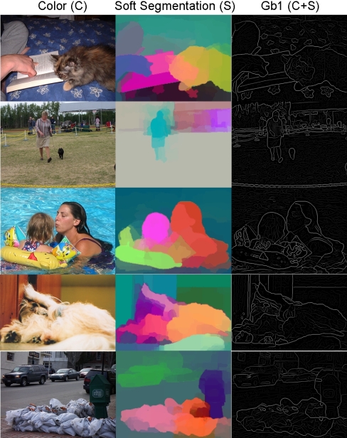
In this section we present a novel method to rapidly generate soft figure/ground image segmentations. Its soft continuous output is similar to the eigenvectors computed by normalized cuts [21] or the soft figure/ground assignment obtained by alpha-matting [12], but it is much faster than most existing segmentation methods. We describe it here because it serves as a fast mid-level interpretation of the image that significantly improves accuracy over raw color alone.

While we describe our approach in the context of color information, the proposed method is general enough to handle a variety of other types of low-level information as well. The method is motivated by the observation that regions of semantic interest (such as objects) can often be modeled with a relatively uniform color distribution. Specifically, we assume that the colors of any image patch are generated from a distribution that is a linear combination (or mixture) of a finite number of color probability distributions belonging to the regions of interest/objects in the image.

Let $\mathbf{c}$ be an indicator vector associated with some patch from the image, such that $c_{i}=1$ if color $i$ is present in the patch and $0$ otherwise. If we assume that the image is formed by a composition of regions of uniform color distributions, then we can consider $\mathbf{c}$ to be a multi-dimensional random variable drawn from a mixture (linear combination) of color distributions $\mathbf{h}_{i}$ corresponding to the image regions:

$$\mathbf{c}\sim\sum_{i}\pi_{i}\mathbf{h}_{i}.$$ (4)

The linear subspace of color distributions can be automatically discovered by performing PCA on collections of such indicator vectors $\mathbf{c}$, sampled uniformly from the image. This idea deserves a further in-depth discussion but, due to space limitations, in this paper we outline just the main idea, without presenting our detailed probabilistic analysis.

Once the subspace is discovered using PCA, for any patch sampled from the image and its associated indicator vector $\mathbf{c}$, its generating distribution (considered to be the distribution of the foreground) can be reconstructed from the linear subspace using the usual PCA reconstruction approximation: $\mathbf{h_{F}(c)\approx h_{0}+\sum_{i}(c-h_{0})}^{T}\mathbf{v_{i}}$. The distribution of the background is also obtained from the PCA model using the same coefficients, but with opposite sign. As expected, we obtain a background distribution that is as far as possible (in the subspace) from the distribution of the foreground: $\mathbf{h_{B}(c)\approx h_{0}-\sum_{i}(c-h_{0})}^{T}\mathbf{v_{i}}$.

Using the figure/ground distributions obtained in this manner, we classify each point in the image as either belonging or not to the same region as the current patch. If we perform the same classification procedure for $n_{s}$ ($\approx 150$) locations uniformly sampled on the image grid, we obtain $n_{s}$ figure/ground segmentations for the same image. At a final step, we again perform PCA on vectors collected from all pixels in the image; each vector is of dimension $n_{s}$ and corresponds to a certain image pixel, such that its $i$-th element is equal to the value at that pixel in the $i$-th figure/ground segmentation. Finally we perform PCA reconstruction using the first $8$ principal components, and obtain a set of $8$ soft-segmentations which are a compressed version of the entire set of $n_{s}$ segmentations. These soft-segmentations are used as input layers to our boundary detection method, and are similar in spirit to the normalized cuts eigenvectors computed for $gPb$ [1].

In Figure 5 we show examples of the first three such soft-segmentations on the RGB color channels. This method takes less than $3$ seconds in MATLAB on a 3.2GHz desktop computer for a $300\times 200$ color image.

5 Experimental analysis

To evaluate the generality of our proposed method, we conduct experiments on detecting boundaries in image, video and RGB-D data on both standard and new datasets. First, we test our method on static color images for which we only use the local color information. Second, we perform experiments on occlusion boundary detection in short video clips. Multiple frames, closely spaced in time, provide significantly more information about dynamic scenes and make occlusion boundary detection possible, as shown in recent work [22, 24, 20, 9]. Third, we also experiment with RGB-D images of people and show that the depth layer can be effectively used for detecting occlusions. In the fourth set of experiments we use the CPMC method [4] to generate figure/ground category segments on the PASCAL2011 dataset. We show how it can be effectively used to generate image layers that can produce high-quality boundaries when processed using our method.

5.1 Boundaries in Static Color Images

Table 1: Comparisons of accuracy (F-measure) and computational time between our method and two other popular methods on BSDS dataset. We use two versions of the proposed method: Gb1 (S) uses color and soft-segmentations as input layers, while Gb1 uses only color. Color layers are represented in CIE Lab space.

Algorithm	Gb1 (S)	Gb1	Gb2	Pb [15]	Canny [3]
F-measure	0.67	0.65	0.64	0.65	0.58
Time (sec)	8	3	2	20	0.1

We evaluate our proposed method on the well-known BSDS300 benchmark [15]. We compare the accuracy and computational time of Gb with $Pb$ [15] and Canny [3] edge detector. All algorithms use only local information at a single scale. Canny uses brightness information, Gb uses brightness and color, while $Pb$ uses brightness, color and texture information. Table 1 summarizes the results. Note that our method is much faster than $Pb$ (times are averages in Matlab on the same $3.2$ GHz desktop computer). When no texture information is used for $Pb$, its accuracy drops significantly while the computational time remains high ($\approx 16$ seconds).

5.2 Occlusion Boundaries in Video

Table 2: Performance comparison on the CMU Motion Dataset of current techniques for occlusion boundary detection.

Algorithm	F-measure
Gb1	0.63
He et al. [9]	0.47
Sargin et al. [20]	0.57
Stein et al. [22]	0.48
Sundberg et al. [24]	0.62

Occlusion boundary detection is an important problem and has received increasing attention in computer vision. Current state-of-the-art techniques are based on the computation of optical flow combined with a global processing phase [22, 24, 20, 9]. We evaluate our approach on the CMU Motion Dataset [22] and compare our method with published results on the same dataset (summarized in Table 2). Optical flow is an important cue for detecting occlusions in video; we use Sun et al.’s publicly available code [23]. In addition to optical flow, we provided Gb-1 with two additional layers: color and our soft segmentation (Section 4). In contrast to the other methods [22, 24, 20, 9], which require significant time for processing and optimization, Gb requires less than $4$ seconds on average (aside from the external optical flow routine) to process images ($230\times 320$) from the CMU dataset.

5.3 Occlusion Boundaries in RGB-D Video

Figure 6: Example results of Gb1 using different input layers: a) color and soft-segmentation on BSDS300; b) color, soft-segmentation and optical flow on CMU Motion Dataset; c) color and depth from RGB-D images.

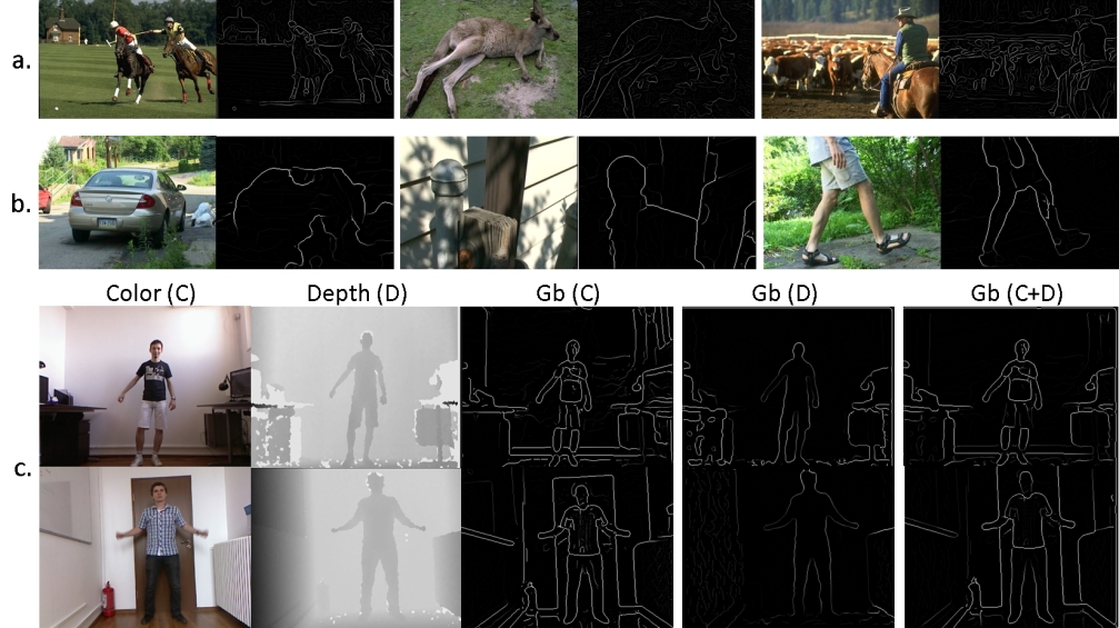
The third set of experiments uses RGB-D video clips of people performing different actions. We combine the low-level color and depth input with large-displacement optical flow [2], which is useful for large inter-frame body movements. Figure 1 shows an example of the input layers and the output of our method. The depth layer was pre-processed to retain the largest connected component of pixels at a similar depth, so as to cover the main subject performing actions. Table 3 summarizes boundary detection in RGB-D on our dataset of $74$ training and $100$ testing images. We see that Gb can effectively combine information from color (C), optical flow (OF) and depth (D) layers to achieve better results. Figure 6) shows sample qualitative results for Gb using only the basic color and depth information (without pre-processing of the depth layer). Without optical flow, the total computation time for boundary detection is less than $4$ seconds per image in MATLAB.

Table 3: Average F-measure on $100$ test RGB-D frames of Gb1 algorithm, using different layers: color (C), depth (D) and optical flow (OF). The performance improves as more layers are combined. Note: the reported time for C+OF and C+D+OF does not include that of generating optical flow using an external module.

Layers	C+OF	C+D	C+D+OF
F-measure	0.41	0.58	0.61
Time (sec)	5	4	6

5.4 Boundaries from soft-segmentations

Our previous experiments use our soft-segmentation method as one of the input layers for Gb. In all of our experiments, we find the mid-level layer information provided by soft-segmentations significantly improves the accuracy of Gb.

The PCA reconstruction procedure described in Section 4 can also be applied to a large pool of figure/ground segments, such as those generated by the CPMC method [4]. This enables us to achieve an F-measure of $0.70$ on BSDS300, which matches the performance of $gPb$ [1]. CPMC+Gb also gives very promising results on the PASCAL2011 dataset, as evidenced by the examples in Figure 7. These preliminary results indicate that fusing evidence from color and soft-segmentation using Gb is a promising avenue for further research.

Figure 7: Qualitative results using Gb on PASCAL2011 images, from color and soft-segmentations obtained from the output of CPMC [4]. Best viewed on the screen.

6 Conclusions

We present Gb, a novel model and algorithm for generalized boundary detection. Our method effectively combines multiple low- and high-level interpretation layers of an input image in a principled manner to achieve state-of-the-art accuracy on standard datasets at a significantly lower computational cost than competing methods. Gb’s broad real-world applicability is demonstrated through qualitative and quantitative results on detecting semantic boundaries in natural images, occlusion boundaries in video and object boundaries in RGB-D data. We also propose a second, even more efficient variant of Gb, with asymptotic computational complexity that is linear with image size. Additionally, we introduce a practical method for fast generation of soft-segmentations, using either PCA dimensionality reduction on data collected from image patches or a large pool of figure/ground segments. We also demonstrate experimentally that our soft-segmentations are valuable mid-level interpretations for boundary detection.

References

- [1] P. Arbelaez, M. Maire, C. Fawlkes, and J. Malik. Contour detection and hierarchical image segmentation. IEEE Transactions on Pattern Analysis and Machine Intelligence, 33(5), 2011.
- [2] T. Brox, C. Bregler, and J. Malik. Large displacement optical flow. In Proceedings of Computer Vision and Pattern Recognition, 2009.
- [3] J. Canny. A computational approach to edge detection. IEEE Transactions on Pattern Analysis and Machine Intelligence, 8(6):679–698, 1986.
- [4] J. Carreira and C. Sminchisescu. Constrained parametric min-cuts for automatic object segmentation. In Proceedings of Computer Vision and Pattern Recognition, 2010.
- [5] A. Cumani. Edge detection in multispectral images. Computer Vision, Graphics, and Image Processing, 53(1), 1991.
- [6] S. Di Senzo. A note on the gradient of a multi-image. Computer Vision, Graphics, and Image Processing, 33(1), 1986.
- [7] P. Dollar, Z. Tu, and S. Belongie. Supervised learning of edges and object boundaries. In Proceedings of Computer Vision and Pattern Recognition, 2006.
- [8] B. Hariharan, P. Arbelaez, L. Bourdev, S. Maji, and J. Malik. Semantic contours from inverse detectors. In Proceedings of International Conference on Computer Vision, 2011.
- [9] X. He and A. Yuille. Occlusion boundary detection using pseudo-depth. In Proceedings of European Conference on Computer Vision, 2010.
- [10] T. Kanade. Image understanding research at CMU. In Image Understanding Workshop, 1987.
- [11] M. Koschan and M. Abidi. Detection and classification of edges in color images. Signal Processing Magazine, Special Issue on Color Image Processing, 22(1), 2005.
- [12] A. Levin, D. Lischinski, and Y. Weiss. A closed form solution to natural image matting. In Proceedings of Computer Vision and Pattern Recognition, 2006.
- [13] J. Mairal, M. Leordeanu, F. Bach, M. Hebert, and J. Ponce. Discriminative sparse image models for class-specific edge detection and image interpretation. In Proceedings of European Conference on Computer Vision, 2008.
- [14] D. Marr and E. Hildtreth. Theory of edge detection. In Proceedings of Royal Society of London, 1980.
- [15] D. Martin, C. Fawlkes, and J. Malik. Learning to detect natural image boundaries using local brightness, color, and texture cues. IEEE Transactions on Pattern Analysis and Machine Intelligence, 26(5), 2004.
- [16] J. Prewitt. Object enhancement and extraction. In Picture Processing and Psychopictorics, pages 75–149. Academic Press, New York, 1970.
- [17] X. Ren. Multi-scale improves boundary detection in natural images. In Proceedings of European Conference on Computer Vision, 2008.
- [18] L. Roberts. Machine perception of three-dimensional solids. In J. Tippett et al., editors, Optical and Electro-Optical Information Processing, pages 159–197. MIT Press, 1965.
- [19] M. Ruzon and C. Tomasi. Edge, junction, and corner detection using color distributions. IEEE Transactions on Pattern Analysis and Machine Intelligence, 23(11), 2001.
- [20] M. Sargin, L. Bertelli, B. Manjunath, and K. Rose. Probabilistic occlusion boundary detection on spatio-temporal lattices. In Proceedings of International Conference on Computer Vision, 2009.
- [21] J. Shi and J. Malik. Normalized cuts and image segmentation. IEEE Transactions on Pattern Analysis and Machine Intelligence, 22(8):888–905, 2000.
- [22] A. Stein and M. Hebert. Occlusion boundaries from motion: Low-level detection and mid-level reasoning. International Journal of Computer Vision, 82(3), 2009.
- [23] D. Sun, S. Roth, and M. Black. Secrets of optical flow estimation and their principles. In Proceedings of Computer Vision and Pattern Recognition, 2010.
- [24] P. Sundberg, T. Brox, M. Maire, P. Arbelaez, and J. Malik. Occlusion boundary detection and figure/ground assignment from optical flow. In Proceedings of Computer Vision and Pattern Recognition, 2011.