Approximate Recall Confidence Intervals

Abstract

Recall, the proportion of relevant documents retrieved, is an important measure of effectiveness in information retrieval, particularly in the legal, patent, and medical domains. Where document sets are too large for exhaustive relevance assessment, recall can be estimated by assessing a random sample of documents; but an indication of the reliability of this estimate is also required. In this article, we examine several methods for estimating two-tailed recall confidence intervals. We find that the normal approximation in current use provides poor coverage in many circumstances, even when adjusted to correct its inappropriate symmetry. Analytic and Bayesian methods based on the ratio of binomials are generally more accurate, but are inaccurate on small populations. The method we recommend derives beta-binomial posteriors on retrieved and unretrieved yield, with fixed hyperparameters, and a Monte Carlo estimate of the posterior distribution of recall. We demonstrate that this method gives mean coverage at or near the nominal level, across several scenarios, while being balanced and stable. We offer advice on sampling design, including the allocation of assessments to the retrieved and unretrieved segments, and compare the proposed beta-binomial with the officially reported normal intervals for recent TREC Legal Track iterations.

Webber, W., Approximate recall confidence intervals

This work was supported in part by the Australian Research Council. This material is based upon work supported by the National Science Foundation under Grant No. 1065250. Any opinions, findings, and conclusions or recommendations expressed in this material are those of the authors and do not necessarily reflect the views of the National Science Foundation.

Author’s address: College of Information Studies, University of Maryland, College Park, MD 20742, The United States of America. Email: wew@umd.edu.

1 Introduction

There are many ways to measure the effectiveness of the retrieval of a set of documents from a document corpus. One of these is recall, the proportion of the relevant documents in the corpus that are retrieved. High recall is important for domains that require comprehensive retrieval, including patent search, medical literature reviews, and document discovery for civil litigation (or e-discovery). To calculate recall, however, we must know the number of relevant documents, or yield, of the corpus. Most corpora are too large for exhaustive relevance assessment; in some cases, even the retrieved documents are too numerous. Retrievals in the Legal Interactive Task of TREC can be in the tens or even hundreds of thousands [Oard et al. (2008)], and document productions in practicing e-discovery can readily run to the hundreds of thousands, extracted from corpora in the millions of documents [Roitblat et al. (2010)].

Where exhaustive assessment is impractical, the yields of the retrieved and unretrieved segments of the corpus can instead be estimated, by drawing a random sample of documents from each segment, and assessing sampled documents for relevance. The proportion of relevant documents, or prevalence, in the sample gives a point estimate of prevalence in the segment, and hence of yield and recall (Section 2.1). Retrieved and unretrieved segments can be sampled at different rates, and each segment may be stratified, taking advantage of auxiliary evidence about stratum prevalence to improve estimator accuracy (Section 2.2).

Point estimates, however, are subject to sampling error; random variability in the proportion of relevant documents sampled in each segment may lead them to under- or overestimate recall. Errors in the point estimate can cause incorrect decisions being made; for instance, a production in e-discovery may be accepted as sufficiently thorough when it is in fact seriously incomplete. Moreover, from the point estimate alone, one cannot tell how likely these erroneous results are to occur. Larger samples lead to more accurate estimates, but this is not expressed in the point estimate, removing much of the incentive for more thorough evaluation.

Errors in point estimates are particularly serious where segments are large and prevalence is low. Such a condition frequently applies to the unretrieved segment of the corpus, since the retrieval will only return a fraction of the corpus but will (if effective) have concentrated relevant documents in this fraction, leaving them sparse in the larger remnant. Small samples may find no relevant documents in the unretrieved segment, leading to the misleading impression of perfect recall. Indeed, when retrieval implementors evaluate their own work, using the point estimate can create a perverse incentive to reduce sample size, so as to minimize the risk of finding an unretrieved relevant document.

Instead of relying on point estimates alone, an interval may be calculated within which recall falls, with $1-\alpha$ confidence. A two-tailed confidence interval provides a finite upper and lower bound, while a one-tailed interval give a lower or an upper bound alone; this paper examines two-tailed intervals. An exact confidence interval, constructed from the sampling distribution of the statistic, guarantees that for any true parameter, at least $1-\alpha$ of resampled and recalculated intervals would cover that parameter. Where exact intervals are unavailable, or too complex to compute or analyze, approximate intervals may be used instead [Smithson (2002)]. In addition, exact intervals often over-cover (provide mean coverage greater than $1-\alpha$) discrete statistics (Section 2.5), whereas approximate intervals may give nominal mean coverage (Section 2.6). This article considers approximate intervals.

We examine several confidence intervals on recall (Section 3). The first treats recall as a binomial proportion on relevant documents (Section 3.1) [Simel et al. (1991)], but assumes the set of relevant documents is sampled at an equal rate. A second method, previously employed in e-discovery [Oard et al. (2008)], uses a normal approximation, a maximum-likelihood estimate (MLE) of variance, and the propagation of error (Section 3.2); but this method often under-covers recall. The remaining methods are new.

For extreme prevalence, the Normal MLE interval underestimates uncertainty, and its assumption of symmetry is incorrect. Adjusting the normal approximation, by adding one or two to the positive and negative sample counts, gives a superior binomial confidence interval [Agresti and Coull (1998), Greenland (2001)]. We apply a similar adjustment to the normal approximation of the recall interval (Section 3.3). The adjustment improves coverage in some circumstances, but has mixed overall accuracy.

The normal intervals assume that recall is approximately normal in its sampling distribution; but this is not in general the case (Section 2.4). A closer approximation models sampled recall as a function of the ratio between two binomial variables. We adapt an interval on a binomial ratio [Koopman (1984)] to bound recall in Section 3.4. The method is generally accurate, but has no finite population adjustment, and so overstates the interval where sample size is a substantial proportion of a segment.

The above intervals are derived from the sampling distribution of recall or its components, such as yield. An alternative, Bayesian approach is to infer a distribution over recall (Section 2.7), and take the $\alpha/2$ and $1-\alpha/2$ quantiles as the interval. We infer distributions over retrieved and unretrieved yield, and generate from these a Monte Carlo estimate of the recall quantiles [Buckland (1984), Chen and Shao (1999)].

A beta posterior with the Jeffreys prior gives accurate intervals on the binomial proportion [Brown et al. (2001)] (Section 2.6), and beta posteriors on retrieved and unretrieved yield generate mostly accurate intervals on recall (Section 3.5). However, the beta interval become less accurate as sample proportion grows, even with a finite population adjustment, as it omits the dependence between what is seen in the sample and what remains in the population.

Sampling without replacement from a finite binomial population is most precisely modelled by a hypergeometric distribution. The conjugate distribution (Section 2.7) to the hypergeometric is the beta-binomial. Our final approach derives beta-binomial posteriors on retrieved and unretrieved yield (Section 3.6), and is the most accurate of those considered. The uniform and the information-theoretic most conservative prior (Section 2.8) are slightly, and differently, unbalanced; a simple prior that sets the beta-binomial hyperparameters to $0.5$ (the half prior) gives best results.

The recall interval methods are evaluated in Section 4 against four criteria: first, mean coverage should be close to $1-\alpha$; second, the standard error of the coverage around this point should be low; third, an equal proportion of uncovered parameters should fall below as above the interval; and fourth, interval width should be the minimum required to achieve accurate mean coverage. These criteria must be evaluated over true parameter distributions, and we define three such distributions or scenarios (Section 4.1): a broad neutral one; a second that emulates an e-discovery environment; and a third that explores the finite population case of a small population and large sample. The beta-binomial with half prior is found to be the most accurate method on all three scenarios.

Section 4.3 examines experimental design, including the allocation of assessments to retrieved and unretrieved segments, and the effect of sample size on interval width. In Section 4.4, we calculate beta-binomial intervals on TREC Legal Interactive participants, and compare them with the officially reported, normal approximation intervals. Finally, Section 5 summarizes our findings, and lays out future work.

2 Preliminaries

This section sets out preliminary materials, used in Section 3 to design recall confidence intervals. We begin by deriving a point estimate of recall (Section 2.1), then extend it to stratified sampling (Section 2.2). The hypergeometric, binomial, and normal distributions, used to construct recall intervals, are introduced in Section 2.3. The point estimate of recall is found in Section 2.4 to be strongly biased, and its sampling distribution highly non-normal, for a representative scenario. Section 2.5 defines exact confidence intervals, while Section 2.6 describes approximate intervals, and why they can be preferable to exact ones. Bayesian prior and posterior distributions are introduced in Section 2.7, and Section 2.8 describes the beta-binomial distribution, which is conjugate prior to the hypergeometric distribution. Interval estimation through Monte Carlo simulation is examined in Section 2.9. Finally, Section 2.10 explains the propagation of error, used for normal intervals, and derives a propagation of error expression for recall. (The reader may wish to skim this section on first reading, and refer back to it to clarify components of the intervals described in Section 3.)

Notation. Symbol Meaning Notes $N_{*}$ Size of corpus $N_{1}$ Size of retrieved segment $N_{0}$ Size of unretrieved segment $N_{*}=N_{1}+N_{0}$ $R_{*}$, $R_{1}$, $R_{0}$ Number of relevant documents (yield) in above populations $R_{*}=R_{1}+R_{0}$ $\pi_{*}$, $\pi_{1}$, $\pi_{2}$ Prevalence of relevant documents in population $\pi=R_{*}/N_{*}$ $n_{*}$, $n_{1}$, $n_{0}$ Size of samples $n_{*}=n_{0}+n_{1}$ $r_{*}$, $r_{1}$, $r_{0}$ Number of relevant documents (yield) in sample $r_{*}=r_{1}+r_{0}$ $p_{*}$, $p_{1}$, $p_{2}$ Prevalence of relevant documents in sample $p_{*}=r_{*}/n_{*}$ $N$, $n$, $R$, $\ldots$ Population size, sample size etc. for unspecified segments $N_{s}$, $n_{s}$, $R_{s}$, $\ldots$ Population size, sample size etc. for stratum $s$ (Section 2.2)

2.1 Estimating recall

Document counts in a retrieval. Relevant Not relevant Retrieved $R_{1}$ $N_{1}-R_{1}$ $N_{1}$ Not retrieved $R_{0}$ $N_{0}-R_{0}$ $N_{0}$ $R_{*}$ $N_{*}-R_{*}$ $N_{*}$

A set retrieval returns from a corpus the set of documents that it considers relevant. Such a retrieval is equivalent to a binary classification of the corpus documents into relevant and irrelevant classes. Let the number of documents in the corpus be $N_{*}$, the number in the retrieved segment be $N_{1}$, and the number in the unretrieved segment be $N_{0}=N_{*}-N_{1}$. Some $R_{*}$ of documents in the corpus are actually relevant to the topic; $R_{1}$ of these fall in the retrieved segment, and $R_{0}$ in the unretrieved segment. Our notation is laid in Table 2, and the document counts are summarized in Table 2.1. We refer to the number of relevant documents in a set as the set’s yield. The recall of a retrieval is the proportion of relevant documents retrieved:

$$\mathrm{Rec}=\frac{R_{1}}{R_{*}}=\frac{R_{1}}{R_{1}+R_{0}}$$ (1)

Corpus yield is rarely known in advance, and the corpus is generally too large to determine it by exhaustive assessment; even the retrieval may be too large to be exhaustively assessed. Instead, a sample-based estimate may be made. A size-$n$ (without-replacement) simple random sample from a population of $N$ elements is one in which each subset of $n$ items has the same probability $1/{N\choose n}$ of being the sample, and each element therefore has $n/N$ probability of being included in the sample [Särndal et al. (1992)]. To estimate recall, we draw a simple random sample of documents from the retrieved and unretrieved segments; assess these documents for relevance; and use the assessed sample to estimate yield in each segment. Let $n_{1}$ and $n_{0}$ be the number sampled from the retrieved and unretrieved segments, and $r_{1}$ and $r_{0}$ be the number relevant in these samples. The prevalence of relevant documents in the retrieved sample, $p_{1}$, is an estimator of prevalence in the retrieved population, ${\pi}_{1}$:

$$p_{1}=\widehat{\pi}_{1}=r_{1}/n_{1}\;,$$

and likewise for the unretrieved sample prevalence, $p_{0}$, on the unretrieved segment. Then, estimators for the yields of the each segment are:

$$\widehat{R}_{1}=N_{1}\widehat{\pi}_{1}\quad;\quad\widehat{R}_{0}=N_{0}\widehat{\pi}_{0}\;;$$

and an estimator for recall is:

$$\widehat{\mathrm{Rec}}=\frac{\widehat{R}_{1}}{\widehat{R}_{1}+\widehat{R}_{0}}=\frac{\widehat{R}_{1}}{\widehat{R}_{*}}\;.$$ (2)

There is an obvious dependence between the numerating sample variable $\widehat{R}_{1}$ and the denominating sample variable $\widehat{R}_{*}=\widehat{R_{1}}+\widehat{R_{0}}$, since the latter includes the former; such dependence makes estimation of variance more complicated (Section 2.10). The dependence can be avoided by rewriting the recall estimator as:

$$\widehat{\mathrm{Rec}}=\frac{1}{1+\widehat{R}_{0}/\widehat{R}_{1}}\;.$$ (3)

As an estimation of a function of a ratio, the recall estimator is biased; that is, $\mathbb{E}[\widehat{\mathrm{Rec}}]\neq\mathrm{Rec}$, the expectation of the estimator does not equal true recall [Hartley and Ross (1954), Cochran (1977)]. The bias is negligible for mediate prevalences and large samples, but can be serious for extreme prevalences and small sample sizes (Section 2.4).

2.2 Stratified sampling

The retrieved and the unretrieved segments can be subdivided into disjoint strata, from each of which a simple random sample is drawn. Estimate accuracy is improved by stratification if prevalence differs between strata, and further still if more samples are allocated to strata that have mediate prevalence, and therefore higher sample variance [Thompson (2002)]. If several set retrievals are being evaluated over the one corpus, the intersections between them form natural strata [Tomlinson et al. (2007)].

The estimated yield $R_{s}$ of stratum $s$ is derived from the size of the stratum $N_{s}$ and the proportion of the stratum sample $r_{s}/n_{s}$ that is relevant:

$$\widehat{R}_{s}=N_{s}r_{s}/n_{s}\;.$$ (4)

The estimated yield of segment $T$ is the sum of the estimated yields of the strata in $T$:

$$\widehat{R}_{T}=\sum_{s\in T}\widehat{R}_{s}\;.$$ (5)

Recall is estimated using these segment estimates in Equation 2.

2.3 Hypergeometric, binomial, and normal distributions

A segment or stratum can be viewed as a binomial population of relevant and irrelevant documents. If we draw a simple random sample of $n$ documents from a population of size $N$, in which $R$ documents are relevant, then the probability that the number $r$ of relevant documents in the sample takes on a particular value $k$ is given by the hypergeometric distribution:

$$\Pr(r=k\,|\,N,R,n)\;=\;f(k)\;=\;\frac{{R\choose k}{N-R\choose n-k}}{{N\choose n}}\;,$$ (6)

where ${a\choose b}=a!/(b!(a-b)!)$. The hypergeometric distribution is so named because its successive terms in $k$ follow a hypergeometric series, in which $f(k+1)/f(k)=g(k)$, where $g(\cdot)$ is some “simple” function of $k$. The prefix “hyper” comes from viewing this as an extension of the geometric series, where $g(\cdot)$ is a constant. Setting $g(k)=k$ and $f(0)=1$ gives the exponential series. For the hypergeometric distribution, we have:

$$g(k)=\frac{(R-k)(n-k)}{(k+1)(N-R-n+k+1)}$$ (7)

See dutka84:ahes for an historical perspective.

As population size $N$ increases, the change that each draw makes upon the original population prevalence $\pi=N/R$ diminishes, and the probability of sampling $k$ relevant documents is approximated with increasing closeness by the binomial distribution:

$$\Pr(r=k\,|\,\pi,n)={n\choose k}\pi^{k}(1-\pi)^{n-k}\;.$$ (8)

The approximation is weaker for smaller populations $N$, larger samples $n$, and prevalences $\pi$ more divergent from $0.5$. For large $n$ and $\pi$ not close to $0$ or $1$, the binomial distribution is in turn approximated by the normal distribution:

$$\Pr(r=k\,|\,\pi,n)=\phi(k;n\pi,n\pi(1-\pi))\;,$$ (9)

where $\phi(\cdot;\mu,\sigma^{2})$ is the normal distribution function with mean $\mu$ and variance $\sigma^{2}$.

Figure 1: Probability of drawing $k$ relevant documents in simple random sample of size $n$ from a population with $N$ documents, $R$ of them relevant, as calculated by the hypergeometric distribution and by the binomial and normal approximations, for different $n$, $N$, and $R$. The normal approximation uses continuity correction; that is, $\Pr(r=k)=\Pr(r<k+0.5)-\Pr(r<k-0.5)$.

Figure 1 compares the hypergeometric, binomial, and discretized normal distributions, for the one population prevalence $R/N=\pi=0.3$ and different population and sample sizes, $N$ and $n$. The hypergeometric is the correct without-replacement sampling distribution. Where $n$ is not small relative to $N$ (left), the binomial and normal approximations overstate the probability of sample prevalence $p$ diverging from population prevalence $\pi$. For small $n$ and $N\gg n$ (middle), the binomial approximation is close to the hypergeometric, but the (incorrectly symmetric) normal approximation overstates the probability of sample prevalence being towards $0.5$. Increasing $n$, while holding $n/N$ fixed (right), brings the normal approximation closer to the hypergeometric [Feller (1945), Nicholson (1956)].

2.4 The sampling distribution and bias of the recall estimator

Example scenario used in Figure 2. Segment Yield Population size Sample size Retrieved $1{,}000$ $2{,}000$ $100$ Unretrieved $3{,}000$ $100{,}000$ $100$ Total $4{,}000$ $102{,}000$ $200$

Figure 2: Sampling distribution of recall for example scenario (Table 2.4). The bars show sampling distributions induced by $r_{1}$ over different values of $r_{0}$. The full distribution is approximated by a Gaussian kernel density estimate. If $r_{0}=0$, estimated recall is precisely $1$; the density here is for comparison of area only. True recall, $R$, and estimator mean, $\bar{\widehat{R}}$, are marked; the estimator has a strong positive bias. A normal curve with the mean and standard deviation of the sampling distribution is also shown.

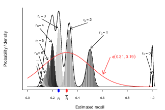
Deriving a closed-form expression for the sampling distribution of recall is not straightforward; but the distribution for any particular population and sample size can be calculated by brute force. Figure 2 shows the sampling distribution of the recall estimator (Equation 2) for a representative scenario, given in Table 2.4. The small number of discrete values that $r_{0}$ can take on, combined with estimator’s skew, produces a complex, skewed, multi-modal distribution, having wide gaps around high recall estimates. The normal distribution, also shown in Figure 2, is a poor approximation.

Figure 3: Bias of recall estimator for scenario described in Table 2.4 but with varying unretrieved sample sizes ($x$ axis) and unretrieved yield (and therefore prevalence). Recall and precision are held fixed in the first three cases by scaling retrieved population size and yield by the same amount as unretrieved yield; in the fourth case, retrieved yield and population size is held fixed, and recall increases with the decrease in unretrieved yield. Note the log scale on the $x$ axis.

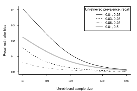
The recall estimator also has a strong positive bias for this scenario: true recall is $0.25$, but the mean of the estimator is $0.31$. The bias is the result of the estimator’s skew, clearly visible in Figure 2; this is one occasion in which the bias in the estimation of a ratio is non-negligible. Figure 3 shows the relationship between estimator bias, unretrieved prevalence, and recall. Bias is greater for low prevalence, small sample size, and low recall.

2.5 Exact confidence intervals

Instead of a point estimate on recall, we can provide an interval within which recall falls with a given confidence. Let $C(X)$ be a function that takes a sample statistic $X$ and produces an interval $[\underline{\theta},\overline{\theta}]$ on some population parameter $\theta$ (such as recall), and let $P_{\theta}$ be the probability distribution over $X$ for a given value of $\theta$. Then $C(x)$ (where $x$ is a realization of $X$) is a $100*(1-\alpha)$ confidence interval if:

$$P_{\theta}\{\theta\in C(X)\}\geq 1-\alpha\;,$$ (10)

for all possible values of $\theta$ [Lehmann and Romano (2005)]. Note that this equation does not state that there is a $1-\alpha$ probability that $\theta$ lies within the calculated confidence interval. In the frequentist understanding, $\theta$ is fixed, not random, and either lies in the interval, or does not. What is random is the sample, $X$; and Equation 10 states that, whatever the actual value of $\theta$, if we repeatedly drew random samples and calculated the confidence interval $C(\cdot)$, then (in the limit) at least $1-\alpha$ of these intervals would cover $\theta$. We refer to $P_{\theta}\{\theta\in C(X)\}$ as the coverage of $\theta$ by the confidence interval.

Finite $\underline{\theta}$ and $\overline{\theta}$ give a two-tailed confidence interval. Such intervals are often built from a pair of inverted, one-tailed hypothesis tests. Let $x$ be the observed sample statistic, and $S_{l}(x;\alpha/2)$ be the interval $[\theta_{l},\infty]$ of null hypotheses $\theta_{0}$ that we accept at significance level $\alpha/2$ in a lower-tailed hypothesis test, given $x$; and let $S_{u}(x;\alpha/2)$ be the corresponding upper-tailed interval $[\infty,\theta_{u}]$. Then a $1-\alpha$ confidence interval is defined as $S_{l}(x;\alpha/2)\cap S_{u}(x;\alpha/2)=[\theta_{l},\theta_{u}]$. Informally, the lower end of the confidence interval is the smallest value of $\theta$ that a lower-tailed hypothesis test fails to reject, given the observed statistic $x$, at level $\alpha/2$, and conversely for the upper end. We refer to an interval constructed by the inversion of hypothesis tests that are based on the distribution of the sample statistic as an exact confidence interval.

Figure 4: Coverage of the exact binomial confidence interval, with a nominal confidence level of 95%, for a sample size of $20$, across different population prevalences. Discontinuities are shown in gray.

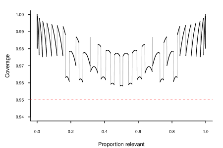
A confidence interval is a tight one if ${P_{\theta}\{\theta\in C(X)\}=1-\alpha}$ for all $\theta$. Exact intervals are not always tight, and exact intervals on discrete sample distributions such as the binomial generally are not [Neyman (1935)]. One such exact interval is the Clopper-Pearson exact binomial confidence interval on a binomial proportion, formed from a pair of inverted, one-tailed binomial significance tests [Clopper and Pearson (1934)]. Figure 4 shows the coverage of the Clopper-Pearson interval at confidence level 95%, across different population prevalences, for a sample size of $20$. The interval achieves coverage of at least $1-\alpha$ for all $\theta$, but does not give tight coverage; average coverage is 97.7%, and is closer to 99% for non-mediate prevalences. (The discontinuities in the coverage of this and subsequently diagrammed intervals are due to the discrete nature of the sample statistic; as we vary the population prevalence, particular counts of positive instances in the sample change from providing intervals that cover the population prevalence to intervals that do not, and vice versa.)

2.6 Approximate confidence intervals

Exact confidence intervals can be difficult to calculate or analyze, and are conservative for discrete distributions. Approximate intervals can be easier to analyze; moreover, while exact intervals guarantee minimum nominal ($1-\alpha$) coverage, approximate intervals can provide average coverage at the nominal level, which is preferable for some applications. (lk09:jos use the term “coverage intervals” for intervals aiming at mean, rather than guaranteed, nominal coverage.)

The approximate Wald interval on a binomial proportion calculates the upper and lower bounds as quantiles of a normal distribution centered upon the sample proportion. This is equivalent to inverting two one-sided normal (Wald) tests, with standard error estimated from sample prevalence [Agresti and Coull (1998)]. If a size $n$ sample produces sample prevalence $p=r/n$, then sample variance is estimated as:

$$\widehat{\mathrm{Var}}_{p}=\frac{p(1-p)}{n}\;.$$ (11)

(This is a biased estimator; the unbiased estimate has $(n-1)$ as its divisor [Cochran (1977), Chapter 3]; however, Equation 11 is in almost universal use, and is used throughout this article.) The standard error $s$ is the square root of this variance, and the confidence interval is $p\pm s\cdot z_{\alpha/2}$, where $z_{\alpha/2}$ is the $\alpha/2$ quantile of the standard normal cumulative distribution function (for instance, $z_{0.05/2}=1.96$).

Figure 5: Coverage of the Wald binomial confidence interval, with a nominal confidence level of 95%, for a sample size of $20$, across different population prevalences. Discontinuities are shown in gray.

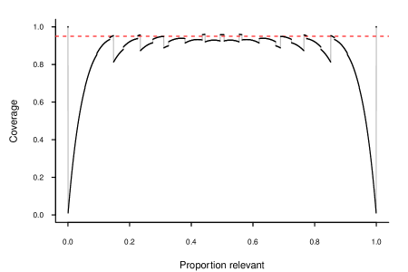
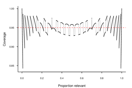
The Wald interval provides poor coverage, as shown in Figure 5, where mean coverage is 85.1%, and coverage drops close to 0 for edge cases. The exact interval is asymmetric when $p\neq 0.5$, as populations with more extreme prevalences have lower sampling error than populations with less; but the Wald interval is always symmetric. For example, the Wald interval for a sample prevalence of $0$ is $[0,0]$, even though a zero prevalence sample can be produced from a population with non-zero prevalence.

Figure 6: Coverage of the Wilson binomial confidence interval, with a nominal confidence level of 95%, for a sample size of $20$, across different population prevalences. Discontinuities are shown in gray.

The Wilson (or score) interval on the binomial also inverts normal hypothesis tests, but uses the prevalences at the candidate lower and upper bounds to estimate standard errors. Thus, the lower half of the interval is shorter than the upper for $p<0.5$, and vice versa for $p>0.5$, as with the exact interval. The precise formula is:

$$\frac{p+(z_{\alpha/2}^{2}/2n)\pm z_{\alpha/2}\sqrt{[p(1-p)+z_{\alpha/2}^{2}/4n]/n}}{1+z_{\alpha/2}^{2}/n}$$ (12)

[Agresti and Coull (1998)]. The coverage of the Wilson interval for our example scenario is shown in Figure 6. Mean coverage here is 95.3%.

ac98:tas show that a 95% Wilson confidence interval is closely approximated by adding two to the count of positive and of negative items observed in the sample, to form an adjusted sample size $\tilde{n}=n+4$ and sample prevalence $\tilde{p}=(r+2)/\tilde{n}$, and using the adjusted $\tilde{p}$ and $\tilde{n}$ in the Wald interval, to produce an interval of:

$$\tilde{p}\pm z_{0.025}\sqrt{\tilde{p}(1-\tilde{p})/\tilde{n}}\;.$$ (13)

More generally, $z_{\alpha/2}^{2}/2$ positive and $z_{\alpha/2}^{2}/2$ negative observations are added, where $z_{\alpha/2}$ is the appropriate quantile of the standard cumulative normal distribution.

2.7 Prior and posterior distributions

An alternative approach to confidence intervals is offered by the Bayesian viewpoint. Here, the true parameter is treated as a random variable, due to the incompleteness of our subjective knowledge of its value. We posit a distribution over the parameter, which describes our subjective belief about the parameter’s likely values, prior to observing the evidence of a sample. The prior distribution is updated from the observed evidence to form a posterior distribution, expressing our belief given the evidence [Gelman et al. (2004)]. A $1-\alpha$ confidence interval can be derived by reading off the $\alpha/2$ and $1-(\alpha/2)$ quantiles of the cumulative posterior distribution. (Such intervals are known as “credible intervals” in Bayesian statistics [Bolstad (2007)].)

Let $\theta$ be the parameter of interest, and $x$ the evidence observed (say, a sample statistic). Given a prior probability distribution $p(\theta)$ on $\theta$, we wish to infer a posterior distribution $p(\theta\,|\,x)$, given observation $x$. Using Bayes’ rule, the posterior is re-written as:

$$p(\theta\,|\,x)=\frac{p(x\,|\,\theta)p(\theta)}{p(x)}=\frac{p(x\,|\,\theta)p(\theta)}{\int p(x\,|\,\theta)p(\theta)\,\mathrm{d}\theta}\;.$$ (14)

That is, the posterior probability of $\theta$ given $x$ is the prior probability of $\theta$, times the likelihood of $x$ given $\theta$, divided by the marginal probability of $x$, derived by integrating over our prior distribution on $\theta$ [Gelman et al. (2004)].

For computational and analytic convenience, it is common to choose the prior distribution $p(\theta)$ from a family of distributions such that the posterior, $p(\theta\,|\,x)$, is from the same family, given the distribution of the likelihood, $p(x\,|\,\theta)$. We say in this case that the distribution of the prior is conjugate to that of the likelihood. For instance, the beta distribution, $\mathit{Beta}(\alpha,\beta)$, with probability distribution function:

$$f(q;\alpha,\beta)=\frac{\Gamma(\alpha+\beta)}{\Gamma(\alpha)\Gamma(\beta)}q^{\alpha-1}(1-q)^{\beta-1}$$ (15)

is conjugate prior to the binomial. ($\Gamma(\cdot)$ is the gamma function; for positive integer $n$, $\Gamma(n)=(n-1)!$.) We use $f(q;\alpha,\beta)$ to express the prior probability $\Pr(\pi=q)$ that the true prevalence $\pi$ is $q$. If the $n$-size sample contains $r$ positive instances, and $n-r$ negative instances, then the prior distribution over $\pi$ of $\mathit{Beta}(\alpha,\beta)$ is updated to the posterior distribution of $\mathit{Beta}(\alpha+r,\beta+n-r)$.

Figure 7: Coverage of the binomial confidence interval based upon a Jeffreys prior, with a nominal confidence level of 95%, for a sample size of $20$, across different population prevalences. Discontinuities are shown in gray.

A particular prior distribution is instantiated from a family by the choice of hyperparameters, such as $\alpha$ and $\beta$ for the beta distribution. In the absence of previous information about $\theta$, a non-informative prior is generally chosen, one which is non-committal about the value of $\theta$. A simple approach for a single parameter of finite range is to choose hyperparameters that give a uniform prior distribution over $\theta$, making each value equiprobable. Setting $\alpha=\beta=1$ achieves this for the beta prior. The uniform prior, however, may be too strong; for small samples of unbalanced binomial populations, it may pull inferences on prevalence $\pi$ too far towards $\pi=0.5$.

A more formally derived prior is the Jeffreys prior, which is the distribution proportional to (for a single parameter) the square root of the parameter’s expected Fisher information (a measure of the mean squared error of an estimator, which is invariant to parameter transformations, such as converting $\pi$ to a logit scale [Jeffreys (1946)]). The Jeffreys prior for the binomial is $\mathit{Beta}(0.5,0.5)$; after observing $r$ positive and $n-r$ negatives, the resulting posterior is $\mathit{Beta}(0.5+r,0.5+n-r)$.

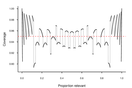
Figure 7 shows the coverage of a 95% Jeffreys interval for a sample size of $20$; mean coverage here is 95.1%. (As the beta is a continuous distribution in the range $[0,1]$, the lower quantile is always greater than $0$, and the upper less than $1$; we adjust the interval by setting its lower end to $0$ if $r=0$, and the upper end to $1$ if $r=n$). Along with the Wilson (Section 2.6), the Jeffreys interval has been recommended as giving the best two-sided coverage for the binomial [Brown et al. (2001), Agresti and Coull (1998)]. The one-sided Wilson interval is biased in $p$ (the lower-bound interval under-covers for low $p$, and over-covers for high $p$); the Jeffreys interval avoids this bias [Liu and Kott (2009)].

2.8 Beta-binomial as prior to hypergeometric

Sampling without replacement from a finite binomial population is most precisely modelled by the hypergeometric distribution, the conjugate prior to which is the beta-binomial. We express the prior probability, $\Pr(R=s)$, that the yield $R$ of a population of size $N$ is $s$, as $\mathit{BetaBin}(\alpha,\beta;N)$, having the probability distribution function:

$$g_{1}(s;N,\alpha,\beta)={N\choose s}\frac{B(s+\alpha,N-s+\beta)}{B(\alpha,\beta)}\;,$$ (16)

where $B(x,y)$ is the beta function, $\Gamma(x)\Gamma(y)/\Gamma(x+y)$. Having sampled $n$ elements and observed $r$ positives, the posterior distribution on $R$ is:

$$g_{p}(s\,|\,r;N,n,\alpha,\beta)={N-n\choose s-r}\frac{B(s+\alpha,N-s+\beta)}{B(\alpha+r,\beta+n-r)}\;,s=r,r+1,\ldots,N-n+r\;.$$ (17)

Note that $g_{p}(s\,|\,r;N,n,\alpha,\beta)=g_{1}(s-r;N-n,\alpha+r,\beta+n-r)$, establishing conjugacy.

As with the beta prior to the binomial, setting $\alpha=\beta=1$ gives a (discrete) uniform prior for $R$ over $[0\cdots N]$; but again, this may be too strong for small samples from unbalanced populations. A weaker prior (which we will refer to as the half prior) sets $\alpha=\beta=0.5$, as with the Jeffreys prior to the binomial, though without the same theoretical justification: since the discrete distribution of the yield $s$ is not differentiable, the Fisher information of the prior cannot be calculated [Berger et al. (2008)].

An alternative non-informative prior is the most conservative prior, which maximizes the expected information gain from the observed data, as measured by the Kullback-Leibler divergence between prior and posterior distributions [Dyer and Chiou (1984)]. dp93:cstm show that the expected information gain for the beta-binomial prior to the hypergeometric is:

$$\begin{gathered}\bar{D}_{\mathrm{BB}}(\alpha,\beta;N,n)=\frac{\Gamma(\alpha+\beta)}{\Gamma(\alpha)\Gamma(\beta)\Gamma(\alpha+\beta+N))}\\ \times\sum_{x=0}^{n}\sum_{r=x}^{N-n+x}{n\choose x}{N-n\choose r-x}\Gamma(\alpha+r)\Gamma(\beta+N-r)\\ \times\ln\left[\frac{{N-n\choose r-x}\Gamma(\alpha)\Gamma(\beta)\Gamma(\alpha+\beta+n)}{{N\choose r}\Gamma(\alpha+x)\Gamma(\beta+n-x)\Gamma(\alpha+\beta)}\right]\;\end{gathered}$$ (18)

(correcting Equation 3.1.3 of dp93:cstm, which has ${n\choose x}$ instead of ${N\choose r}$ in the final line). dp93:cstm also demonstrate that Equation 18 is concave and symmetric in $\alpha$ and $\beta$, so the maximum occurs where $\alpha=\beta$. Finding the value $\alpha=\beta$ which maximizes Equation 18 provides the most conservative prior [Dyer and Pierce (1993)]. We solve Equation 18 as an optimization problem; solutions fall in the range $[0.1,1.0]$. The double sum in Equation 18 makes it $O(Nn)$ to calculate, while for large $N$ and mediate $n/N$, the solution in $\alpha=\beta$ appears to converge; we therefore limit $N$ to $1000$ and $n$ to $1000-\min(N-n,200)$.

The most conservative prior has anomalous behavior for tiny sample sizes. For $n=1$, the prior hyperparameters collapse to $0$, and the posterior distribution to $p(s)=1$, where $s=0$ if the sampled element is negative, and $s=N$ if positive. For $n>1$ but still small, the prior likewise tends to be too weak. The potential for this to lead to inaccurate interval coverage is observed empirically in Section 4.

2.9 Monte Carlo estimation of intervals

Bayesian confidence intervals are taken from the quantiles of the posterior cumulative distribution of the parameter being bounded. The posterior on recall is a function of beta or beta-binomial posteriors (Sections 3.5 and 3.6) on segment yield; deriving a closed-form expression for the combined distribution is not straightforward. One could instead calculate the probabilities of all $(N_{0}+1)\cdot(N_{1}+1)$ yield combinations, and the recall for each; sort by recall; and then accumulate probabilities from each end until the desired quantiles are achieved. This is $O(N^{2})$ in both time and memory.

Instead of exhaustive computation, we estimate the interval by Monte Carlo simulation [Buckland (1984), Chen and Shao (1999)]. The beta or beta-binomial posteriors on retrieved and unretrieved yield are independent, and can be efficiently sampled from [Cheng (1978)]. We draw $s$ such samples in pairs, one from the posterior of each segment, and calculate the recall for each sample. These $s$ recall values are sorted, and the $\alpha/2$ and $1-\alpha/2$ quantiles taken as estimates of the like quantiles of the distribution, and hence of the interval. For the methods described in Sections 3.5 and 3.6, we employ $40{,}000$ draws; this takes around $50$ milliseconds on a current single processor.

2.10 Propagation of error

The Wald and similar approximate intervals are calculated from a normal distribution centered on the point estimate; the spread of the distribution depends on the sampling error of the statistic. If the sample statistic is a function of other statistics, the variance of the approximation is likewise a function of the component variances. If a random variable $X$ is a function of other random variables $A$ and $B$, written:

$$X=f(A,B)\;,$$ (19)

then, by the theory of propagation of error:

$$\mathrm{Var}(X)=\left(\frac{\partial f}{\partial A}\sigma_{A}\right)^{2}+\left(\frac{\partial f}{\partial B}\sigma_{B}\right)^{2}+2\left|\frac{\partial f}{\partial A}\frac{\partial f}{\partial B}\right|\mathrm{Cov}_{AB}\;,$$ (20)

where $\sigma_{Y}=\sqrt{\mathrm{Var}(Y)}$ is the standard deviation of $Y$, $\mathrm{Cov}_{YZ}$ is the covariance between $Y$ and $Z$, and $\left|Y\right|$ is the absolute value of $Y$ [Taylor (1997)].

The recall estimate in Equation 3 is a function of the variables $\widehat{R}_{1}$ and $\widehat{R}_{0}$. Since $\widehat{R}_{0}$ and $\widehat{R}_{1}$ are sampled from distinct segments, they are independent (unlike $\widehat{R}_{1}$ and $\widehat{R}_{*}$ in Equation 2), so the covariance term in Equation 20 is $0$. It can be shown that:

$$\frac{\partial\widehat{\mathrm{Rec}}}{\partial\widehat{R}_{0}}=-\frac{1}{\widehat{R}_{1}\left(1+\widehat{R}_{0}/\widehat{R}_{1}\right)^{2}}\;,$$ (21)

and that:

$$\frac{\partial\widehat{\mathrm{Rec}}}{\partial\widehat{R}_{1}}=\frac{\widehat{R}_{0}}{\left(\widehat{R}_{1}+\widehat{R}_{0}\right)^{2}}\;.$$ (22)

Applying Equation 20, we find that:

$$\widehat{\mathrm{Var}}(\widehat{\mathrm{Rec}})=\frac{\widehat{\mathrm{Var}}(\widehat{R}_{1})\widehat{R}_{0}^{2}+\widehat{\mathrm{Var}}(\widehat{R}_{0})\widehat{R}_{1}^{2}}{(\widehat{R}_{1}+\widehat{R}_{0})^{4}}\;,$$ (23)

where:

$$\widehat{\mathrm{Var}}(\widehat{R}_{1})=N_{1}^{2}\cdot\widehat{\mathrm{Var}}_{p_{1}}\cdot\left(1-\frac{n_{1}}{N_{1}}\right)\;,$$ (24)

and similarly for $\widehat{\mathrm{Var}}(\widehat{R}_{0})$; note the finite-population adjustment in the last term. A maximum likelihood estimate (MLE) of $\widehat{\mathrm{Var}}_{p_{1}}$ may be taken from Equation 11. For stratified sampling, the segment estimate variance is the sum of stratum estimate variances (Equation 24 with stratum values). legal08:trec propagate error from Equation 2, instead of Equation 3, while ignoring the covariance term in Equation 20. This naive estimate overstates recall variance by including $\widehat{\mathrm{Var}}(\widehat{R}_{1})$ twice.

3 Recall confidence intervals

Recall confidence intervals. Name Section Summary Coverage Naive binomial 3.1 Treat sensitivity as binomial proportion sampled from true positives. Very inaccurate in most conditions. Normal MLE 3.2 Normal approximation with maximum-likelihood variance estimate, aggregated by propagation of error. Unstable; biased for very low prevalences or heavy samples. Normal Laplace 3.3 Add one to positive and negative sample counts in each segment, then as per Normal MLE. Slightly less unstable and biased than Normal MLE. Normal Agresti-Coull 3.3 Add two to sample counts, then as per Normal MLE. As unstable and biased as Normal MLE. Koopman 3.4 Monotonic decreasing transform of interval on ratio between binomial variables. Biased to overcoverage for heavy samples; otherwise accurate. Beta Jeffreys 3.5 Infer beta posteriors from Jeffreys priors on segments; Monte Carlo generation of recall distribution; take quantiles of generated distribution. Biased to undercoverage for heavy samples; otherwise accurate. Beta-binomial Uniform 3.6 Infer beta-binomial posteriors from uniform priors on segments; then as per Beta Jeffreys. Slightly unstable for very low prevalences, marginally understates recall; otherwise accurate. Beta-binomial MCP 3.6 Infer beta-binomial posteriors from most conservative priors on segments; then as per Beta Jeffreys. Slightly unstable, overstates recall in some conditions; otherwise accurate. Beta-binomial Half 3.6 Infer beta-binomial posteriors from priors with hyperparameters $\alpha=\beta=0.5$ on segments; then as per Beta Jeffreys. Accurate in all conditions examined.

Using the techniques laid out in Section 2, this section proposes nine recall intervals, summarized in Table 3 (coverage results n the fourth column look forward to Section 4). The first four methods use normal approximations; the fifth, an analytic interval on a ratio between binomials; and the last four, Bayesian segment posteriors (the first from the beta prior to the binomial, and the next three from beta-binomial priors to the hypergeometric) and Monte Carlo simulation.

3.1 Sensitivity as a binomial proportion

The sensitivity of a diagnostic procedure, like the recall of a classifier, is the proportion of positive instance correctly identified. ssm91:jclep treat sensitivity as a binomial proportion on the population of true positives, and infer a Wald interval on this proportion (Section 2.6), to give a $1-\alpha$ recall (or sensitivity) confidence interval of:

$$\widehat{\mathrm{Rec}}\pm z_{\alpha/2}\cdot\sqrt{\widehat{\mathrm{Rec}}(1-\widehat{\mathrm{Rec}})/n}\;.$$ (25)

We refer to this as the naive binomial interval.

The naive binomial assumes that positive instances are equally sampled, which, though valid in the epidemiological randomized control trials considered by ssm91:jclep, does not generally hold for retrieval recall estimation, since the retrieved and unretrieved segments may be sampled separately, and at different rates. The same inequality in sampling rate means the interval extends poorly to stratified sampling.

3.2 Normal with maximum-likelihood variance

The sampling variance of recall can be derived from segment yield variance by error propagation (Equation 23), and standard error is the square root of variance:

$$\widehat{s}_{R}=\sqrt{\widehat{\mathrm{Var}}(\widehat{\mathrm{Rec}})}$$

If we assume that $\widehat{\mathrm{Rec}}$ is normally distributed, and has equal variance along its range, then a $1-\alpha$ confidence interval is:

$$\widehat{\mathrm{Rec}}\pm z_{\alpha/2}\cdot\widehat{s}_{\mathrm{R}}\;.$$ (26)

Note that the interval is centered on the recall point estimate. A direct estimate of $\mathrm{Var}(\widehat{\mathrm{Rec}})$ uses $\widehat{\mathrm{Var}}_{p}=p(1-p)/n$ (Equation 11) in Equation 24. We refer to the approximate normal interval with this estimates as the Normal MLE method. Stratified sampling is handled by summing stratum variances, as described in Section 2.10.

The Normal-MLE method has two problems. First, the sampling distribution of recall may diverge from the normal (Section 2.4); for instance, recall is bounded by the range $[0,1]$, whereas the normal distribution is unbounded. And second, the MLE of $\mathrm{Var}(\widehat{R})$ is biased low for extreme sample prevalence. In particular, if $p_{0}=0$, then $\widehat{\mathrm{Var}}(\widehat{R}_{0})$ is $0$ and the recall interval is $1\pm 0$, but perfect recall is certainly not assured.

3.3 Laplace and Agresti-Coull adjustments to the normal

ac98:tas adjust the Wald confidence interval on the binomial proportion by adding $2$ to the count of positive and negative sample instances (Section 2.6). A similar idea can be applied to the interval on recall, by adding $1$ or $2$ to the positive and negative sample counts in the retrieved and unretrieved segments. We denote the addition of $2$ as the Agresti-Coull adjustment, and of $1$ as the Laplace adjustment (from Laplace’s prior to the binomial) [Agresti and Caffo (2000), Greenland (2001)]. In stratified sampling, the adjustment would be applied to each stratum.

If $c$ is the amount of the adjustment, then the adjusted proportion relevant for each segment or stratum, $\tilde{p}=(r+c)/(n+2c)$, is used in Equation 11 to derive an adjusted expression for $\widehat{\mathrm{Var}}_{p}$ in Equation 24 [Agresti and Coull (1998)]:

$$\widetilde{\mathrm{Var}}_{p}=\frac{\tilde{p}(1-\tilde{p})}{n+2c}\;.$$ (27)

The adjusted variance expression is then propagated through Equation 23, with adjusted estimators of retrieved and unretrieved yield:

$$\tilde{R}_{1}=N_{1}\tilde{p}_{1}\quad;\quad\tilde{R}_{0}=N_{0}\tilde{p}_{0}\;,$$ (28)

to calculate an adjusted variance ($\widetilde{\mathrm{Var}}(\widehat{\mathrm{Rec}})$) and standard error ($\tilde{s}_{\mathrm{R}}=\widetilde{\mathrm{Var}}(\widehat{\mathrm{Rec}})^{1/2}$) for recall. The midpoint for the interval is also calculated with the adjusted counts:

$$\widetilde{\mathrm{Rec}}=\frac{\tilde{R}_{1}}{\tilde{R}_{1}+\tilde{R}_{0}}\;.$$ (29)

And finally, the adjusted interval is estimated with these adjusted values:

$$\widetilde{\mathrm{Rec}}\pm z_{\alpha/2}\cdot\tilde{s}_{\mathrm{R}}\;.$$ (30)

These adjustments make the interval more robust to extreme sample prevalences. We force the top end of the confidence interval to $1$ if there are no positives in the unretrieved sample, and the bottom to $0$ if none in the retrieved.

3.4 Ratio between binomial proportions: Koopman

koopman84:biom derives an approximate confidence interval on the ratio of two independent binomial proportions, which he refers to as the chi-square method. (The equations are too lengthy to reproduce here; see Section 2.2 of koopman84:biom for details.) The formula for recall in Equation 3 is a monotonically decreasing function of the ratio between the independent binomial proportions $\widehat{R}_{0}$ and $\widehat{R}_{1}$. Therefore, a $1-\alpha$ confidence interval on the latter ratio will also be a $1-\alpha$ confidence interval on recall, with ends reversed [Smithson (2002)]. We refer to this as the Koopman interval. We set the lower bound to $0$ if there are no relevant documents in the retrieved sample, and the upper bound to $1$ if there are no relevant documents in the unretrieved sample. The method does not have a straightforward extension to stratified sampling, since the compound samples from retrieved and unretrieved segments cease being simple binomial random samples.

3.5 Ratio between beta posteriors with Jeffreys priors

A beta posterior based on a Jeffreys prior provides a binomial confidence interval with good coverage (Section 2.7). The method can be adapted to derive an interval on recall. Beta posteriors are inferred on the prevalences of the retrieved and unretrieved segments, $\pi_{1}$ and $\pi_{0}$. A pair of independent observations, $\pi_{1}^{*}$ and $\pi_{0}^{*}$, is drawn from these posteriors, and the yields for the corresponding segments are calculated. For instance, for the retrieved segment:

$$\pi_{1}^{*}\leftarrow\mathit{Beta}(0.5+r_{1},0.5+n_{1}-r_{1})$$

$$R_{1}^{*}=r_{1}+\pi_{1}^{*}\cdot(N_{1}-n_{1})\;.$$

(Note the adjustment for sample size in $N_{1}-n_{1}$, and for sample yield in $r_{1}$; we have seen a portion of the population in the sample, and do not need to estimate the yield of that portion.) A recall value is then observed from these segment yield estimates. The process is repeated multiple times, and a $1-\alpha$ interval is taken from the $\alpha/2$ and $1-\alpha/2$ quantiles of the resulting Monte Carlo distribution (Section 2.9). The lower bound is forced to $0$ if there are no relevant documents in the retrieved sample, and the upper bound to $1$ if there are none in the unretrieved sample. We refer to this as the Beta Jeffreys recall interval. Stratified sampling is handled by separately deriving posteriors for each stratum, and drawing samples from each such posterior.

3.6 Ratio between beta-binomial posteriors with uniform, most conservative, or half priors

Both Koopman and Beta Jeffreys intervals are based on the binomial distribution. In practice, though, the document population is finite, and the hypergeometric distribution is the more accurate model, the conjugate prior to which is the beta-binomial (Section 2.8). For our final approximate recall interval, beta-binomial posteriors are inferred for the yields of the retrieved and unretrieved segment, $R_{1}$ and $R_{0}$, and a Monte Carlo distribution over recall is generated by drawing paired observations from these posteriors. For instance,

$$R_{1}^{*}\leftarrow\mathit{BetaBin}(\alpha+r_{1},\beta+n_{1}-r_{1})$$

The $\alpha/2$ and $1-\alpha/2$ quantiles of the generated distribution provide a $1-\alpha$ confidence interval on recall.

Section 2.8 considers three choices for the $\alpha$ and $\beta$ hyperparameters to the beta-binomial prior. The first sets $\alpha=\beta=1$, giving a uniform prior (Beta-binomial Uniform). The second selects the information-theoretic most conservative prior for the population and sample size (Beta-binomial MCP). And the third mimics the Jeffreys prior to the binomial, by setting $\alpha=\beta=0.5$ (Beta-binomial Half). Stratified sampling is handled by drawing from posteriors on each stratum; the greater number and smaller size of strata emphasizes the importance of careful prior choice. The lower bound is forced to $0$ if there are no relevant documents in the retrieved sample, and the upper bound to $1$ if there are none in the unretrieved sample.

4 Evaluation

This section provides the experimental evaluation of the intervals described in Section 3. Intervals are tested for their coverage of three representative retrieval or classification estimation scenarios (Section 4.1); the beta-binomial posterior with half prior is found to give the most unbiased, balanced, and stable coverage of the methods considered (Section 4.2). We offer advice on sampling design, the allocation of assessments to retrieved and unretrieved segments, and the interval widths that can be expected (Section 4.3). Finally, we calculate half-prior beta-binomial intervals for participants in the Interactive Task of the Legal Track in TREC 2008 and TREC 2009, and compare them with the officially reported, normal approximation intervals (Section 4.4).

4.1 Evaluation methodology

We propose four criteria for evaluating the coverage of an approximate (two-tailed) confidence interval:

Unbiasedness

Is mean coverage at the nominal (that is, $1-\alpha$) level?

Consistency

Is variability in coverage small?

Balance

Do non-covered parameter values fall below and above the interval with equal frequency?

Narrowness

Subject to the other criteria, is the interval width narrow?

An interval satisfying the above criteria will be described as accurate.

With no constraint on width, a method that gave an interval of $[0,1]$ 95% of the time, of $(0,0)$ 2.5% of the time, and of $(1,1)$ 2.5% of the time, would achieve perfect accuracy, satisfying the criteria of unbiasedness, consistency, and balance. Narrow intervals, however, can easily be achieved through inadequate coverage; and unbalanced intervals on asymmetric distributions can be narrower by shifting coverage from the longer to the shorter tail. Therefore, the width criterion is subject to the other criteria.

Scenario variables. Variable Meaning $N_{*}$ Size of population $\pi_{*}=R_{*}/N_{*}$ Proportion relevant in population $\mathrm{Rec}=R_{1}/R_{*}$ Recall of retrieval $\mathrm{Prec}=R_{1}/N_{1}$ Precision of retrieval $n_{1}$ Size of sample from retrieved segment $n_{0}$ Size of sample from unretrieved segment

The measured accuracy of coverage depends upon the distribution of population parameters. In Section 2.6, we evaluated binomial intervals using a uniform distribution over prevalence, and a fixed sample size. However, the one recall value can result from different combinations of population and retrieved segment size and prevalence, and different sample sizes will provoke different interval behaviors. Exhaustively searching the full parameter space is infeasible (and, for population size, formally impossible), and would obscure behavior in environments of particular interest. Instead, we evaluate recall intervals under different retrieval or classification scenarios, each of which provides distributions over population size, prevalence, and retrieval precision and recall, as well as sample sizes for the retrieved and unretrieved segments.

Table 4.1 lists the scenario variables. A sample from these variables creates a scenario realization. We first determine the characteristics of the population or corpus: the number of documents it contains ($N_{*}$), and the proportion of these documents which are relevance ($p_{*}$). Then, we determine the characteristics of the production or retrieval: the proportion of relevant documents retrieved ($\mathrm{Rec}$), and the proportion of retrieved documents that are relevant ($\mathrm{Prec}$). Finally, we determine the characteristics of the sample: the number of relevant documents sampled from the retrieved ($n_{1}$) and unretrieved ($n_{0}$) segments. All of the values in Table 2 can be calculated from these scenario variables, save the sample outcomes $r_{0}$ and $r_{1}$ themselves. For instance, $N_{1}$, the retrieval segment size, is $\lfloor N\cdot\mathrm{Rec}/\mathrm{Prec}\rceil$ ($\lfloor\cdot\rceil$ is the rounding operator), while $R_{1}$, the number of relevant documents in the retrieved segment, is $\lfloor N\cdot\mathrm{Prec}\rceil$. Coverage of each realization is estimated by drawing repeated samples from the population (simulated by observing a value for $r$ from a $\mathit{HyperGeom}(N,R,n)$ distribution), and counting the proportion of the interval estimates generated from these samples that cover the true recall of the realization.

We define three scenarios using these variables, described below: the neutral, legal, and small scenarios. The neutral scenario (Section 4.1.1) tests a wide range of conditions, avoiding only edge cases of very low corpus prevalence and sample sizes that are a substantial proportion of corpus size. The legal scenario (Section 4.1.2) then tests the large corpus, low-prevalence circumstances encountered in the TREC Legal Track (and many other retrieval tasks), while the small scenario (Section 4.1.3) investigates the finite population case, where sample size is a large proportion of population size.

These three scenarios cover most conditions that are likely to be encountered in sampling for recall estimation on a closed corpus, either in a retrieval or classification context, and test important edge cases that stress the performance of interval estimators. (One might observe larger corpora and larger samples sizes than in the neutral scenario, combined with more mediate prevalence than in the legal scenario, but these are unstressful conditions for any estimator.) Any particular estimation task will have narrower parameters than the intentionally broad ones of these scenarios, and so observe difference distributions of interval accuracy. A system evaluator might employ the evaluation methods presented here to test interval methods in his or her expected estimation environment. Nevertheless, an interval that performs well on all of the realizations of a broad scenario will perform well on any particular narrower subset scenario, while intervals that often perform poorly on the broader case will perform well on only certain of the narrower ones.

4.1.1 Neutral scenario

Neutral scenario. Variable Range Mean Distribution $N_{*}$ $1{,}000$ to $4{,}000{,}000$ $2{,}000{,}500$ $\mathit{Unif}(1e3,4e6)$ $\pi_{*}$ $0.02$ to $0.8$ $0.41$ $\mathit{Unif}(0.02,0.8)$ $\mathrm{Rec}$ $0.1$ to $1.0$ $0.55$ $\mathit{Unif}(0.1,1.0)$ $\mathrm{Prec}$ $0.1$ to $1.0$ $0.64$ $\mathit{Unif}(\min(0.1,0.95\pi_{*},1.05\cdot R_{1}/N_{*}),1.0)$ $n_{1}$ $10$ to $4{,}000$ $1{,}935$ $\mathit{Unif}(10,\min(4000,\lfloor N_{1}/10\rfloor))$ $n_{0}$ $10$ to $4{,}000$ $1{,}995$ $\mathit{Unif}(10,\min(4000,\lfloor N_{0}/10\rfloor))$

The neutral scenario is described in Table 4.1.1; it represents a variety of classification and retrieval tasks, on populations large enough to require sampling. The neutral scenario covers a wide range of population prevalences; very low prevalences are saved for the legal and small scenarios. All levels of precision and recall are considered, apart from those so low as to represent an extremely flawed classification or retrieval. Two lower bounds are set on precision, the first to ensure that retrieved prevalence is not much worse than unretrieved (the retrieval does at least as well as random), and the second to guarantee that not all documents are retrieved. Sample sizes have equal distributions between retrieved and unretrieved segments.

4.1.2 Legal scenario

Legal scenario. Variable Range Mean Distribution $N_{*}$ $500{,}000$ to $50{,}000{,}000$ $1{,}075{,}000$ $$5\text{\times}{10}^{5}$\cdot 10^{\mathit{Unif}(0,2)}$ $\pi_{*}$ $0.003$ to $0.115$ $0.031$ $$2\text{\times}{10}^{-3}$\cdot 1.5^{\mathit{Unif}(1,10)}$ $\mathrm{Rec}$ $0.0025$ to $0.84$ $0.33$ $$2.5\text{\times}{10}^{-3}$\cdot\mathit{Unif}(1,34)^{1.65}$ $\mathrm{Prec}$ $0.025$ to $0.92$ $0.48$ $\mathit{Unif}(\min(0.025,2\cdot R_{1}/N_{*}),0.92)$ $n_{1}$ $20$ to $5{,}120$ $820$ $20\cdot 2^{\mathit{Unif}(0,\max(8,\lfloor\log_{2}(N_{1}/20)\rfloor))}$ $n_{0}$ $100$ to $12{,}800$ $3{,}170$ $100\cdot 2^{\mathit{Unif}(0,\max(7,\lfloor\log_{2}(N_{0}/100)\rfloor))}$

Figure 8: Sorted recall of participants in the Interactive Task of the TREC 2008 and TREC 2009 Legal Track (dots), with fitted line of $$2.5\text{\times}{10}^{-3}$\cdot\mathit{Unif}(1,34)^{1.65}$. Recall scores are sample-based estimates using adjudicated assessments [Oard et al. (2008)].

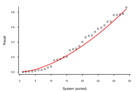
The legal scenario (Table 4.1.2) represents e-discovery and similar large scale retrieval. The distributions of scenario variables are fitted to parameters observed in the TREC 2008 and TREC 2009 Legal Interactive task (Section 4.4). For instance, Figure 8 shows the fit of the recall distribution in Table 4.1.2 to the recall values from the task. The scenario corpus size is large, and prevalence low for a classification (though not for a retrieval) task. A median of 2% of the retrieved segment is sampled, and only 0.5% of the unretrieved. Unretrieved samples will frequently contain few or no relevant documents, testing handling of extreme proportions. The lower bound on precision ensures that no more than half the corpus is retrieved, and also that very low precision is not matched with very high recall—the only relationship observed between the two metrics amongst TREC Legal Interactive participants.

4.1.3 Small scenario

Small scenario. Variable Range Mean Distribution $N_{*}$ $1{,}000$ to $10{,}000$ $5{,}500$ $\mathit{Unif}(1e3,1e4)$ $\pi_{*}$ $0.02$ to $0.22$ $0.12$ $\mathit{Unif}(0.02,0.22)$ $\mathrm{Rec}$ $0.1$ to $1.0$ $0.55$ $\mathit{Unif}(0.1,1.0)$ $\mathrm{Prec}$ $0.025$ to $0.92$ $0.51$ $\mathit{Unif}(\min(0.025,2\cdot R_{1}/N_{*}),0.92)$ $n_{1}$ $20\%$ to $50\%$ of retrieved segment $290$ $N_{1}\cdot\mathit{Unif}(0.2,0.5)$ $n_{0}$ $5\%$ to $30\%$ of unretrieved segment $815$ $N_{0}\cdot\mathit{Unif}(0.05,0.3)$

The small scenario, described in Table 4.1.3, represents a retrieval-style task on a small corpus with a relatively large sample budget. Sample sizes are large relative to population, up to 50% for the retrieved segment, and up to 30% for the unretrieved. Prevalence is allowed to exceed the legal scenario, but is kept below $0.22$, in line with most retrieval tasks. No more than half the population is retrieved.

4.2 Coverage of the three scenarios

We now report the coverage of the nine confidence interval estimators on the three scenarios described above, testing the four criteria established at the start of Section 4: unbiasedness; consistency; balance (in Section 4.2.4); and width (in Section 4.2.5).

4.2.1 Neutral scenario

Figure 9: Interval coverage for the neutral scenario. $1{,}000$ scenario realizations are instantiated, and $1{,}000$ samples drawn for each realization; the same realizations and samples are used for all interval methods. The thick line in each box shows median coverage, the box edges the quartiles. Mean coverage is shown as a cross. Circles show realizations with coverage outside the quartiles by more than $1.5$ times the inter-quartile range. Minimum coverage falling below the range of the graph is marked on the left margin with “$<$”.

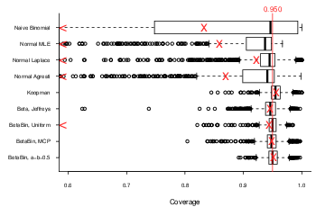
Figure 9 shows the mean and median coverage and coverage consistency of the different interval methods for the neutral scenario. The naive binomial is highly inconsistent and biased low; its assumptions are violated by different retrieved and unretrieved sampling rates (Section 3.1). The MLE normal is biased only slightly low, but is highly unstable, with frequent significant under-coverage; the cause is false symmetry and understatement of variance (Section 3.2), particularly for low prevalence unretrieved samples. The Laplace adjustment corrects the mean bias, and avoids the worst cases of instability, but still has occasions of marked undercoverage, while the Agresti-Coull adjustment is little better than the MLE, suggesting the plus-two adjustment is too large. The remaining five methods are nearly unbiased and more consistent, except that the most-conservative prior to the beta-binomial shows a tendency to occasional undercoverage (the prior is too weak for certain extreme proportions). The Koopman and uniform beta-binomial methods give the tightest behavior.

4.2.2 Legal scenario

Figure 10: Interval coverage for the legal scenario. Other details are as for Figure 11.

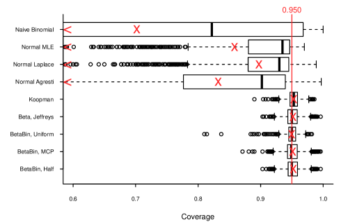
The results for the legal scenario are shown in Figure 10. The naive binomial and normal methods perform much worse than for the neutral scenario, due to the low prevalence, particularly in the unretrieved segment. The Laplace adjustment to the normal only partially corrects bias, while the Agresti-Coull adjustment makes it worse. Analysis shows that under-coverage is due to over-adjustment: unretrieved yield is over-estimated, and hence recall understated. The remaining five methods all give unbiased coverage, though this time the uniform prior to the beta-binomial shows a tendency towards under-coverage, as the uniform prior is too strong for very low prevalences.

4.2.3 Small scenario

Figure 11: Interval coverage for the small scenario. Other details are as for Figure 11.

The results for the small scenario are given in Figure 11. The naive binomial and the three normal methods again show bias and poor consistency, with the Laplace-adjusted normal being the best of them. Unlike the previous scenarios, however, the Koopman and Jeffreys methods are strongly biased. Koopman intervals take no account of the elements already seen, and are too wide; Jeffreys intervals miss the negative dependence between sample and unsampled prevalence, and are too narrow. The beta-binomial posterior methods are largely accurate, with the half prior being (marginally) the most consistent of the three.

4.2.4 Upper and lower gaps

Figure 12: Upper and lower gaps for different CI methods on the neutral scenario. Each underlying data point represents a scenario realization, and states the proportion of the samples drawn from that realization for which recall falls above (or below) the interval estimated from the sample. Realizations and resamples are as for Figure 11. The thick lines shows the median gap, the cross the mean. Box edges are first and third quartiles, while circles show gaps that are outside the quartiles by more than $1.5$ times the inter-quartile range. Methods for which the maximum gap is greater than the range of the graph are marked on the right margin with “$>$”.

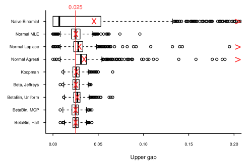
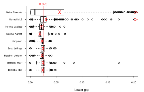
Balance is the third desideratum for intervals. Interval balance for the neutral scenario is shown in Figure 12. The MLE normal method tends to overstate recall (lower gap larger than upper), and the adjusted normal methods to understate it, because they respectively understate and overstate unretrieved prevalence. The uniform prior, though unbiased (Figure 11), tends to understatement; the prior on the unretrieved segment is sometimes too strong. The most conservative prior often overstates recall, while the half prior is more balanced. The legal and small scenarios (not shown for space) give similar results, with the half-prior beta-binomial being consistently the best balanced.

4.2.5 Interval width

Mean width of 95% recall interval for different interval methods on the three scenarios, along with the mean coverage of these methods. Method Neutral Legal Small width cvr width cvr width cvr Naive Binomial 0.05 0.90 0.13 0.70 0.16 0.93 Normal MLE 0.05 0.94 0.23 0.86 0.14 0.93 Normal Laplace 0.05 0.95 0.27 0.90 0.14 0.95 Normal Agresti 0.05 0.95 0.24 0.83 0.14 0.93 Koopman 0.05 0.95 0.27 0.95 0.16 0.97 Beta, Jeffreys 0.05 0.95 0.28 0.95 0.13 0.92 BetaBin, Uniform 0.05 0.95 0.26 0.95 0.14 0.95 BetaBin, MCP 0.05 0.95 0.28 0.95 0.14 0.95 BetaBin, Half 0.05 0.95 0.28 0.95 0.14 0.95

Mean interval width is given in Table 4.2.5, along with mean coverage. The widths of biased intervals tend in the same direction as the interval’s bias, though not universally: the naive binomial method provides an over-wide but under-covering (because highly imbalanced) interval on the small scenario. Unbiased intervals have similar widths; balance and consistency should be used to choose between them.

4.2.6 Discussion

Root mean squared error from nominal coverage for interval estimators on the three different scenarios. Method Scenario Mean Neutral Legal Small Naive Binomial 0.183 0.395 0.117 0.231 Normal MLE 0.043 0.197 0.081 0.107 Normal Laplace 0.012 0.092 0.022 0.042 Normal Agresti 0.022 0.193 0.056 0.090 Koopman 0.007 0.010 0.024 0.014 Beta, Jeffreys 0.008 0.014 0.037 0.020 BetaBin, Uniform 0.007 0.013 0.009 0.010 BetaBin, MCP 0.009 0.015 0.011 0.012 BetaBin, Half 0.008 0.014 0.010 0.010

We summarize the bias and consistency of the examined interval methods in Table 4.2.6, as the root mean squared error (RMSE) between actual and nominal coverage. The naive binomial method is biased and highly inconsistent for all the scenarios considered. The normal methods are less biased, with the Laplace adjustment offering reasonable average performance, but are highly unstable, with coverage often falling far below the nominal level (Figures 9, 10, and 11). These interval methods should be avoided. The Koopman ratio-of-binomial method, and the beta and beta-binomial posterior methods, are more reliable. Where the sample is a large proportion of the population, however, as in the small scenario, the Koopman method leads to over-coverage, and the Jeffreys to under-coverage. The uniform, most conservative, and half priors to the beta-binomial posterior offer similar unbiasedness and consistency, but the former two are less balanced, the uniform understating recall, and the most conservative overstating it (Figure 12). Though there is not a great difference between the performance of the uniform and the half prior to the beta-binomial, the latter is slightly more balanced, and is therefore the recommended interval.

Figure 13: Proportion of scenario realizations for which each interval method gives coverage closest to the nominal level, for each of the evaluation scenarios. Tied coverage (to the fidelity of the simulation, which is $1{,}000$ simulated samples per realization) receives split counts.

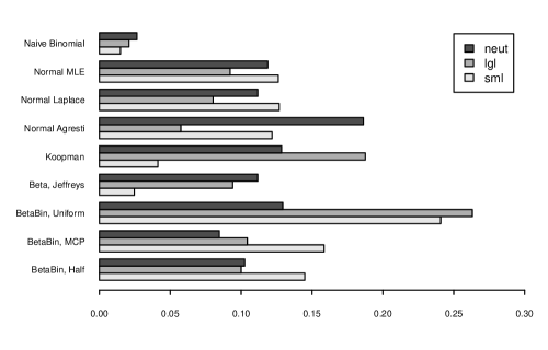
Do methods with better mean accuracy perform better in the most cases? Figure 13 shows that the answer is no. Though the Koopman and posterior methods have as little as a tenth of the RMSE of the normal methods, they outperform only on a moderate majority of individual realizations. And although the most-conservative prior and half prior beta-binomial have similar RMSE to the uniform prior, the uniform prior comes closest to nominal coverage in a plurality of realizations for all three scenarios. The weaker methods underperform not by being slightly less accurate on most cases, but by being much less accurate in particular circumstances. The evaluator, though, cannot tell from the sample precisely which circumstance the population fits into; therefore, the overall most accurate interval is advisable.

4.3 Sampling design and expected intervals

The previous sections have discussed the retrospective analysis of recall confidence intervals. The experimental designer or system auditor, however, is faced with several prospective questions. How wide a confidence interval is an analysis likely to produce? How large a sample size is needed to reduce intervals to reasonable width? And what division of samples between retrieved and unretrieved segments minimizes width?

Figure 14: The width of confidence intervals, using the beta-binomial posterior with half prior, for retrievals of different levels of effectiveness. A sample of $n$ is drawn from the retrieved segment and $5{,}000-n$ documents from the unretrieved segment, from a population of $5{,}000{,}000$ documents, and a retrieved segment size of $500{,}000$.

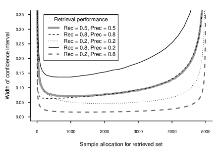
Interval width depends on sample size; division of sample amongst segments; corpus yield; recall; retrieval size; and (though only marginally) population size. Sample size and sample allocation are under the evaluator’s control; retrieval and population size are known at design time; but yield and recall are unknown prior to sampling. The sensitivity of allocation strategies to retrieval performance is examined in Figure 14. Interval width is clearly affected by retrieval quality: low recall and high precision leads to narrow intervals, since prevalence is high and sampling variance low in both retrieved and unretrieved segments. Here, width is not sensitive to allocation. In contrast, low precision and high recall causes wide intervals, and favors an allocation of samples towards the unretrieved segment. A 20%:80% sample allocation to the retrieved and unretrieved segments gives reasonably close to minimal interval width across the scenarios, but would obstruct the accurate estimation of precision.

Figure 15: Width of recall confidence interval for varying sample sizes and different retrieved segment sizes. The population size is $5\text{\times}{10}^{6}$, and the retrieval has recall and precision both $0.5$. Interval widths are shown for the optimal allocation of samples and assessments to the retrieved and unretrieved segments. The black lines show the beta-binomial posterior with half prior. The grey lines show the intervals given by the MLE normal method.

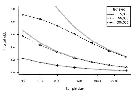
Allocation aside, the chief variable at the evaluator’s control is sample size. Figure 15 shows interval width as a function of sample size for the half-prior beta-binomial and MLE normal methods, assuming an ideal sample allocation between segments. The normal method shows the standard $1/\sqrt{n}$ reduction in interval width with an $n$-fold increase in sample size, but gives overly wide intervals for low prevalence and small samples, producing intervals wider than $1.0$ in some cases. The beta-binomial agrees closely with the normal for high prevalence and large samples, but gives smaller intervals for low prevalence and small samples. Consequently, the decrease in interval width with sample size is slower than $1/\sqrt{n}$ in such circumstances.

4.4 Intervals for TREC Legal Track

We conclude the experimental section by calculating confidence intervals for the Interactive Task of the TREC 2008 and TREC 2009 Legal Track. The task was evaluated using stratified sampling (Section 2.2), with strata defined by the intersection of participant team retrievals; $n$ teams define $2^{n}$ strata, some of which may be empty. Different strata received different sampling rates; in particular, the bottom stratum, of documents retrieved by no system, was sampled only sparsely [Oard et al. (2008)]. The recall confidence interval for the official results was calculated using the Normal-MLE method (Section 3.2), though with a propagation of error expression that omits yield covariance (Section 2.10).

Recall estimates with 95% confidence intervals for the Interactive Task of the TREC 2008 Legal Track. The beta-binomial interval uses the $\alpha=\beta=0.5$ as prior. The normal interval use MLE variance estimates, without and with correction for the correlation between system and corpus yield estimates. Topic Team Recall CI (BBin, 0.5) CI (Norm, uncorr.) CI (Norm, corr.) 2.5% 97.5% 2.5% 97.5% 2.5% 97.5% t102 Ad Hoc Pool 0.314 0.273 0.360 0.266 0.362 0.271 0.358 Clearwell 0.016 0.014 0.018 0.014 0.018 0.014 0.018 Pittsburgh 0.007 0.006 0.008 0.006 0.008 0.006 0.008 t103 H5 0.624 0.580 0.665 0.579 0.668 0.581 0.666 Ad Hoc Pool 0.403 0.374 0.430 0.371 0.434 0.374 0.431 Clearwell 0.158 0.146 0.169 0.146 0.169 0.146 0.169 Buffalo 0.061 0.056 0.066 0.056 0.066 0.056 0.066 Pittsburgh 0.026 0.024 0.028 0.024 0.029 0.024 0.029 t104 Ad Hoc Pool 0.345 0.185 0.577 0.111 0.580 0.143 0.548 Clearwell 0.003 0.002 0.005 0.001 0.004 0.001 0.004

Recall and interval estimates for the Interactive Task of the TREC 2009 Legal Track. The MLE normal and Laplace methods correct for yield estimate correlation.

Topic	Team	Recall		CI (BBin, 0.5)			CI (Norm, corr.)			CI (Laplace)
				2.5%	97.5%		2.5%	97.5%		2.5%	97.5%
t201	UW	0.778		0.451	0.928		0.485	1.070		0.351	0.916
	CS	0.489		0.287	0.592		0.304	0.673		0.226	0.593
	CB	0.204		0.119	0.250		0.126	0.282		0.093	0.247
	UP	0.167		0.097	0.208		0.102	0.231		0.076	0.205
t202	UW	0.673		0.523	0.768		0.542	0.803		0.501	0.771
	CS	0.579		0.451	0.662		0.467	0.692		0.432	0.664
t203	UW	0.865		0.623	0.881		0.832	0.897		0.552	0.940
	UB	0.592		0.427	0.621		0.552	0.631		0.378	0.652
	ZL-NoCull	0.175		0.123	0.185		0.157	0.192		0.105	0.185
	ZL-Cull	0.029		0.019	0.034		0.023	0.035		0.016	0.033
t204	H5	0.762		0.572	0.882		0.595	0.930		0.538	0.874
	UD	0.305		0.229	0.360		0.235	0.374		0.216	0.358
	CB	0.198		0.149	0.240		0.151	0.246		0.140	0.238
t205	CS	0.673		0.592	0.738		0.599	0.747		0.587	0.737
	EQ	0.463		0.404	0.509		0.409	0.516		0.399	0.505
	IN	0.292		0.253	0.327		0.254	0.329		0.250	0.325
t206	CB-High	0.076		0.052	0.112		0.046	0.106		0.049	0.109
	LO	0.042		0.025	0.069		0.020	0.063		0.023	0.067
	CB-Mid	0.011		0.007	0.015		0.007	0.015		0.007	0.014
	CB-Low	0.009		0.006	0.013		0.006	0.013		0.005	0.012
t207	CB	0.768		0.698	0.798		0.723	0.813		0.689	0.802
	UW	0.761		0.688	0.791		0.714	0.807		0.677	0.791
	LO	0.538		0.489	0.566		0.503	0.573		0.484	0.569
	EQ	0.483		0.437	0.507		0.451	0.515		0.430	0.507

Table 4.4 compares the normal and beta-binomial confidence intervals for TREC 2008. The “Ad Hoc Pool” team was a deep pseudo-run made up by pooling the automated runs from a parallel task. The normal intervals use the MLE estimate of variance, and are calculated without and with correction for the correlation between team and corpus yield estimates (Section 2.10); the uncorrected interval estimate is as reported in the official results [Oard et al. (2008)]. The correlation-corrected interval differs substantially from the uncorrected only for the Ad Hoc Pool pseudo-team on Topic 104, since only then does it display the necessary combination of a high-recall, low-precision ($0.023$) run. It is also only on Topic 104 that there is much difference between the corrected MLE normal and the beta-binomial intervals, since the unretrieved segment sample prevalence is not small for the other two topics.

The normal and beta-binomial intervals for TREC 2009 are shown in Table 4.4. Correlation correction is applied for the normal version. The uncorrected intervals (not shown) are marginally narrower in most cases, and sharply narrower for a few. In contrast to the previous year, the normal and beta-binomial intervals generally disagree. The mean absolute difference in width is $13\%$, with the beta-binomial being narrower for all topics save Topic 203. The lower bound of the beta-binomial generally falls below that of the normal, and is wider beneath the point estimate than above it. The cause is low or zero sample prevalence in the bottom stratum, to which the beta-binomial method correctly gives a wider upper than lower bound. The normal method assigns an impossible upper-bound recall of $1.07$, even though the team fails to return several known relevant documents. For comparison, the final two columns of Table 4.4 show the Laplace adjustment to the normal interval (Section 3.3). The adjusted interval is generally left-skewed, like the beta-binomial. The intervals, however, are wider, sometimes substantially so, than the beta-binomial.

5 Conclusion

Several recall confidence interval methods have been considered in this article. The naive binomial method, in which recall is treated as a simple binomial proportion on the relevant documents, assumes equal sampling of retrieved and unretrieved segments, which is not generally the case in retrieval evaluation. The normal approximation, with propagation of per-segment yield sampling error, understates variance on the unretrieved segment, and is strongly biased towards undercoverage. The Laplace and Agresti-Coull adjustments only partially correct this bias, and generalize poorly to stratified sampling. The Koopman analytical ratio-of-binomial estimator gives much better results, as does the ratio-of-binomials posterior to the Jeffreys prior. Both, however, are inaccurate when a large proportion of the population is sampled.

The most accurate approximate interval infers a beta-binomial posterior for each segment or stratum, and samples from this posterior to generate a distribution over recall. The interval is unbiased, with mean coverage at the nominal $1-\alpha$ level, and is stable, with quartiles clustering to within a couple of percentage points of the nominal level. The greatest stability and balance is given by a prior that sets the hyperparameters $\alpha$ and $\beta$ to $0.5$; this is more accurate than either the uniform or the (more theoretically grounded) most-conservative prior. (Our results are summarized in the final column of Table 3, on page 3.)

We have provided guidance on experimental design. Interval width is generally minimized by assigning most assessments to the unretrieved segment, particularly for high-recall retrievals, though such an allocation will be at the cost of wider intervals on precision. Assuming optimal allocation between segments, interval width under the beta-binomial prior method decreases by the usual square root of sample size only once the width of the interval is well below $0.5$; before that, decrease in interval width is slower.

Finally, we have used the half-prior beta-binomial posterior method recommended in this article to produce interval estimates on the TREC 2008 and TREC 2009 Legal Track, Interactive Task participants, and compared them with the unadjusted and adjusted normal methods. In some cases, the normal methods give similar estimates to the beta-binomial; in others, marked differences exist, particularly where sample prevalence in the unretrieved segment is low.

5.1 Future work

This article has considered two-tailed confidence intervals. One-tailed intervals, particularly those setting a lower bound on performance, are also of interest. Achieving accurate one-tailed intervals can be more demanding than for two-tailed intervals, since under-coverage at one end cannot be compensated by over-coverage at the other. For instance, cai05:jspi finds that though the two-tailed Wilson interval on the binomial is highly accurate, the one-tailed interval is systematically biased. lk09:jos find that the beta posterior with Jeffreys prior gives an accurate one-tailed interval on the binomial proportion, and the good balance observed for the two-tailed half-prior beta-binomial interval on recall (Figure 12) suggests that it would also provide an accurate one-tailed interval. This article has also only considered approximate intervals, aiming at nominal mean coverage. In some circumstances, a guaranteed minimal coverage may be required. For such cases, an exact method is needed.

We noted in Section 2.4 that the recall estimator is biased, and that the bias can be severe and positive, particularly where the prevalence of the unretrieved segment is low, and the unretrieved sample size is small. There is long-standing literature on unbiased ratio estimators [Hartley and Ross (1954), Al-Jararha (2008)]. An unbiased estimator of recall is desirable.

It was also noted in Section 2.4 that the sampling distribution of recall is generally asymmetric. For the similarly asymmetric sampling distribution of the binomial proportion, a two-tailed Wald interval on $\operatorname{logit}{\pi}$ of $\ln p/q\pm z/\sqrt{npq}$ has been found to give coverage characteristics similar to the Wilson interval [Newcombe (2001)], as has the one-tailed variant [Liu and Kott (2009)]. Applying such a transform to the normal approximation interval for recall might correct its spurious symmetry. The transformed interval would still mishandle extreme cases, though; for instance, when estimated recall is $0$ or $1$, then the logit-transformed intervals are $[0,0]$ and $[1,1]$, respectively.

The optimal allocation of samples to retrieved and unretrieved segments depends upon prevalence in each set (Section 4.3). Prevalence is not known in advance, but could be estimated during sampling. Additionally, sampling could finish once a certain interval width or lower bound is reached. Such sequential analysis can lead to biased estimates [Wetherill and Glazebrook (1986)]; the degree of this bias would need to be determined.

We have assumed there is no assessor error. Such error has a particularly strong impact on low-prevalence corpora; even a low false positive rate can drastically inflate estimated yield. The error rate can be estimated and corrected by sampling primary assessments for checking by a more authoritative assessor (if available) [Webber et al. (2010)], though this estimate will have its own sampling error, and the authoritative assessor might also make mistakes. Other approaches might overlap multiple assessors, to verify dubious assessments and estimate assessor reliability.

Only simple and stratified random sampling have been considered in this article. A more general approach is unequal sampling, in which each document is assigned its own inclusion probability, based on its probability of relevance and its weight in the evaluation metric. Unequal sampling has been applied in the Ad Hoc Task of the TREC Legal Track [Tomlinson et al. (2007), Hedin et al. (2009)], and methods for unequal sampling and point estimation in ranked retrieval evaluation have been developed [Aslam et al. (2006), Aslam and Pavlu (2008)]. Estimating variance for unequal sampling schemes requires calculating joint inclusion probabilities for sampled pairs. A simple sampling method for which joint inclusion probabilities are known is Sunter sampling [Sunter (1977), Särndal et al. (1992)]; as it happens, the sampling scheme used in the Legal Ad Hoc Task is equivalent to Sunter sampling. pavlu08:phd provides a variance estimator for the average precision metric, though it understates variance by ignoring a component of variance. Such variance estimators, however, rely upon normal approximations to turn into confidence intervals, and handle zero-prevalence samples no better than simple random sampling approaches. Bayesian methods are also more complex to use with unequal sampling, since we are no longer estimating a distribution over a single parameter (such as the proportion relevant in a segment), but require a more complex model linking probability of relevance to rank and other evidence [Carterette (2007)].

Intervals for set-based metrics other than recall, such as precision and F1 score, can be inferred using the same beta-binomial posteriors on segment or stratum yield. The characteristics and accuracy of these intervals need to be established, and compared with other interval methods, particularly for the interval on precision, which (as a simple binomial proportion) has a plethora of intervals available.

Simple or stratified random sampling requires minimal assumptions, and produces wide bounds on yield and recall. Stronger assumptions can give tighter bounds, but shift the uncertainty to the validity of the assumptions. For instance, kkia99:asis propose a capture-recapture model, using the overlap between two runs to estimate yield. In its simplest form, this requires the unrealistic assumption that the two runs are independent; but a model that accounts for run correlation could be developed. z98:sigir fits and extrapolates a model of proportion relevant at depth in ranked retrievals. Extending to depth one million a curve that has been observed to depth one hundred requires some courage, but the approach could be combined with sampling and other forms of evidence. As with simple random sampling, confidence intervals are required as well as point estimates

Whatever estimation methods are used, and even if assessor error is excluded, bounds on recall for large collections with low prevalence and constrained assessment budgets will generally be wide, sometimes so wide as to appear unhelpful to the evaluator. But this is no reason to neglect the calculation and reporting of such bounds; quite the reverse. Where uncertainty is high, it is all the more imperative to reveal that fact. Only once the uncertainty is recognized can the effort be made to bring it within tolerable limits.

*REPRODUCIBLE RESULTS STATEMENT

An implementation of the recall confidence interval methods, along with other code and datasets used in this paper, is available at codalism.com/~wew/w12recci.

The author thanks Doug Oard, Dave Lewis, Eric Slud, and Mossaab Bagdouri, and the anonymous reviewers, for their perceptive suggestions.

August 2012October 2012

References

- Agresti and Caffo (2000) Agresti, A. and Caffo, B. 2000. Simple and effective confidence intervals for proportions and differences of proportions result from adding two successes and two failures. The American Statistician 54, 4, 280–288.
- Agresti and Coull (1998) Agresti, A. and Coull, B. A. 1998. Approximate is better than “exact” for interval estimation of binomial proportions. The American Statistician 52, 2, 119–126.
- Al-Jararha (2008) Al-Jararha, J. 2008. Unbiased ratio estimation for finite populations. Ph.D. thesis, Colorado Statue University.
- Aslam and Pavlu (2008) Aslam, J. and Pavlu, V. 2008. A practical sampling strategy for efficient retrieval evaluation. Tech. rep., Northeastern University.
- Aslam et al. (2006) Aslam, J., Pavlu, V., and Yilmaz, E. 2006. A statistical method for system evaluation using incomplete judgments. In Proc. 29th Annual International ACM SIGIR Conference on Research and Development in Information Retrieval, S. Dumais, E. Efthimiadis, D. Hawking, and K. Järvelin, Eds. Seattle, Washington, USA, 541–548.
- Berger et al. (2008) Berger, J. O., Bernardo, J. M., and Sun, D. 2008. Objective priors for discrete parameter spaces. Tech. rep., Duke University.
- Bolstad (2007) Bolstad, W. M. 2007. Introduction to Bayesian Statistics. John Wiley & Sons.
- Brown et al. (2001) Brown, L. D., Cai, T. T., and DasGupta, A. 2001. Interval estimation for a binomial proportion. Statistical Science 18, 2, 101–133.
- Buckland (1984) Buckland, S. T. 1984. Monte Carlo confidence intervals. Biometrics 40, 3, 811–817.
- Cai (2005) Cai, T. T. 2005. One-sided confidence intervals in discrete distributions. Journal of Statistical Planning and Inference 131, 1, 63–88.
- Carterette (2007) Carterette, B. 2007. Robust test collections for retrieval evaluation. In Proc. 30th Annual International ACM SIGIR Conference on Research and Development in Information Retrieval, C. L. A. Clarke, N. Fuhr, N. Kando, W. Kraaij, and A. de Vries, Eds. Amsterdam, the Netherlands, 55–62.
- Chen and Shao (1999) Chen, M.-H. and Shao, Q.-M. 1999. Monte Carlo estimation of Bayesian credible and HPD intervals. Journal of Computational and Graphical Statistics 8, 1, 69–92.
- Cheng (1978) Cheng, R. C. H. 1978. Generating beta variates with nonintegral shape parameters. Communications of the ACM 21, 4, 317–322.
- Clopper and Pearson (1934) Clopper, C. J. and Pearson, E. S. 1934. The use of confidence or fiducial limits illustrated in the case of the binomial. Biometrika 26, 4, 404–413.
- Cochran (1977) Cochran, W. G. 1977. Sampling Techniques 3rd Ed. John Wiley & Sons.
- Dutka (1984) Dutka, J. 1984. The early history of the hypergeometric function. Archive for History of Exact Sciences 31, 1, 15–34.
- Dyer and Chiou (1984) Dyer, D. and Chiou, P. 1984. An information-theoretic approach to incorporating prior information in binomial sampling. Communications in Statistics: Theory and Methods 13, 17, 2051–2083.
- Dyer and Pierce (1993) Dyer, D. and Pierce, R. L. 1993. On the choice of the prior distribution in hypergeometric sampling. Communications in Statistics: Theory and Methods 22, 8, 2125–2146.
- Feller (1945) Feller, W. 1945. On the normal approximation to the binomial distribution. The Annals of Mathematical Statistics 16, 4, 319–329.
- Gelman et al. (2004) Gelman, A., Carlin, J. B., Stern, H. S., and Rubin, D. B. 2004. Bayesian Data Analysis 2nd Ed. Chapman and Hall/CRC.
- Greenland (2001) Greenland, S. 2001. Agresti, A., and Caffo, B., “Simple and effective confidence intervals for proportions and differences of proportions result from adding two successes and two failures,” The American Statistician, 54, 280–288: Comment by Greenland and reply. The American Statistician 55, 2, 172.
- Guenther (1971) Guenther, W. C. 1971. Unbiased confidence intervals. The American Statistician 25, 1, 51–53.
- Hartley and Ross (1954) Hartley, H. O. and Ross, A. 1954. Unbiased ratio estimators. Nature 174, 270–271.
- Hedin et al. (2009) Hedin, B., Tomlinson, S., Baron, J. R., and Oard, D. W. 2009. Overview of the TREC 2009 legal track. In Proc. 18th Text REtrieval Conference, E. Voorhees and L. P. Buckland, Eds. Gaithersburg, Maryland, USA, 1:4:1–40. NIST Special Publication 500-278.
- Jeffreys (1946) Jeffreys, H. 1946. An invariant form for the prior probability in estimation problems. Proc. Royal Society of London. Series A, Mathematical and Physical Sciences 186, 1007, 453–461.
- Kantor et al. (1999) Kantor, P., Kim, M.-H., Ibraev, U., and Atasoy, K. 1999. Estimating the number of relevant documents in enormous collections. In Proc. ASIS Annual Meeting. 507–514.
- Koopman (1984) Koopman, P. A. R. 1984. Confidence intervals for the ratio of two binomial proportions. Biometrics 40, 2, 513–517.
- Lehmann and Romano (2005) Lehmann, E. L. and Romano, J. P. 2005. Testing Statistical Hypotheses 3rd Ed. Springer.
- Liu and Kott (2009) Liu, Y. K. and Kott, P. S. 2009. Evaluating alternative one-sided coverage intervals for a proportion. Journal of Official Statistics 25, 4, 569–588.
- Newcombe (2001) Newcombe, R. G. 2001. Logit confidence intervals and the inverse sinh transformation. The American Statistician 55, 3, 200–202.
- Neyman (1935) Neyman, J. 1935. On the problem of confidence intervals. The Annals of Mathematical Statistics 6, 3, 111–116.
- Nicholson (1956) Nicholson, W. L. 1956. On the normal approximation to the hypergeometric distribution. The Annals of Mathematical Statistics 27, 2, 471–483.
- Oard et al. (2008) Oard, D. W., Hedin, B., Tomlinson, S., and Baron, J. R. 2008. Overview of the TREC 2008 legal track. In Proc. 17th Text REtrieval Conference, E. Voorhees and L. P. Buckland, Eds. Gaithersburg, Maryland, USA, 3:1–45. NIST Special Publication 500-277.
- Pavlu (2008) Pavlu, V. 2008. Large scale IR evaluation. Ph.D. thesis, Northeastern University.
- Roitblat et al. (2010) Roitblat, H. L., Kershaw, A., and Oot, P. 2010. Document categorization in legal electronic discovery: computer classification vs. manual review. Journal of the American Society for Information Science and Technology 61, 1, 70–80.
- Särndal et al. (1992) Särndal, C.-E., Swensson, B., and Wretman, J. 1992. Model assisted survey sampling. Springer-Verlag.
- Simel et al. (1991) Simel, D. L., Samsa, G. P., and Matchar, D. B. 1991. Likelihood ratios with confidence: sample size estimation for diagnostic test studies. Journal of Clinical Epidemiology 44, 8, 763–770.
- Smithson (2002) Smithson, M. 2002. Confidence intervals. Sage Publications.
- Sunter (1977) Sunter, A. B. 1977. List sequential sampling with equal or unequal probabilities without replacement. Journal of the Royal Statistical Society. Series C (Applied Statistics) 26, 3, 261–268.
- Taylor (1997) Taylor, J. R. 1997. Introduction to error analysis 2nd Ed. University Science Books.
- Thompson (2002) Thompson, S. K. 2002. Sampling 2nd Ed. John Wiley & Sons, New York.
- Tomlinson et al. (2007) Tomlinson, S., Oard, D. W., Baron, J. R., and Thompson, P. 2007. Overview of the TREC 2007 legal track. In Proc. 16th Text REtrieval Conference, E. Voorhees and L. P. Buckland, Eds. Gaithersburg, Maryland, USA, 5:1–34. NIST Special Publication 500-274.
- Webber et al. (2010) Webber, W., Oard, D. W., Scholer, F., and Hedin, B. 2010. Assessor error in stratified evaluation. In Proc. 19th ACM International Conference on Information and Knowledge Management. Toronto, Canada, 539–548.
- Wetherill and Glazebrook (1986) Wetherill, G. B. and Glazebrook, K. D. 1986. Sequential Methods in Statistics 3rd Ed. Chapman and Hall.
- Zobel (1998) Zobel, J. 1998. How reliable are the results of large-scale information retrieval experiments? In Proc. 21st Annual International ACM SIGIR Conference on Research and Development in Information Retrieval, W. B. Croft, A. Moffat, C. J. van Rijsbergen, R. Wilkinson, and J. Zobel, Eds. Melbourne, Australia, 307–314.