A uniform asteroseismic analysis of 22 solar-type stars observed by Kepler

S. Mathur¹¹affiliation: High Altitude Observatory, NCAR, P.O. Box 3000, Boulder, CO 80307, USA , T. S. Metcalfe¹¹affiliation: High Altitude Observatory, NCAR, P.O. Box 3000, Boulder, CO 80307, USA ²²affiliation: Computational & Information Systems Laboratory, NCAR, P.O. Box 3000, Boulder, CO 80307, USA , M. Woitaszek²²affiliation: Computational & Information Systems Laboratory, NCAR, P.O. Box 3000, Boulder, CO 80307, USA , H. Bruntt³³affiliation: Department of Physics and Astronomy, Aarhus University, 8000 Aarhus C, Denmark ⁴⁴affiliation: LESIA, UMR8109, Université Pierre et Marie Curie, Université Denis Diderot, Obs. de Paris, 92195 Meudon Cedex, France , G. A. Verner⁵⁵affiliation: School of Physics and Astronomy, University of Birmingham, Edgbaston, Birmingham B15 2TT, UK , J. Christensen-Dalsgaard¹¹affiliation: High Altitude Observatory, NCAR, P.O. Box 3000, Boulder, CO 80307, USA ³³affiliationmark: , O. L. Creevey⁶⁶affiliation: Laboratoire Lagrange, UMR7293, Université de Nice Sophia-Antipolis, CNRS, Observatoire de la Côte d’Azur, BP 4229, 06304 Nice Cedex 4, France , G. Doğan¹¹affiliation: High Altitude Observatory, NCAR, P.O. Box 3000, Boulder, CO 80307, USA ³³affiliation: Department of Physics and Astronomy, Aarhus University, 8000 Aarhus C, Denmark , S. Basu⁷⁷affiliation: Department of Astronomy, Yale University, P.O. Box 208101, New Haven, CT 06520-8101, USA , C. Karoff³³affiliation: Department of Physics and Astronomy, Aarhus University, 8000 Aarhus C, Denmark ⁵⁵affiliation: School of Physics and Astronomy, University of Birmingham, Edgbaston, Birmingham B15 2TT, UK , D. Stello⁸⁸affiliation: Sydney Institute for Astronomy, School of Physics, University of Sydney, NSW 2006, Australia , T. Appourchaux⁹⁹affiliation: Institut d’Astrophysique Spatiale, UMR8617, Université Paris XI, Batiment 121, 91405 Orsay Cedex, France , T. L. Campante³³affiliation: Department of Physics and Astronomy, Aarhus University, 8000 Aarhus C, Denmark ¹⁰¹⁰affiliation: Centro de Astrofísica and Faculdade de Ciências, Universidade do Porto, Rua das Estrelas, 4150-762 Porto, Portugal , W. J. Chaplin⁵⁵affiliation: School of Physics and Astronomy, University of Birmingham, Edgbaston, Birmingham B15 2TT, UK , R. A. García¹¹¹¹affiliation: Laboratoire AIM, CEA/DSM-CNRS-Université Paris Diderot; IRFU/SAp, Centre de Saclay, 91191 Gif-sur-Yvette Cedex, France , T. R. Bedding⁸⁸affiliation: Sydney Institute for Astronomy, School of Physics, University of Sydney, NSW 2006, Australia , O. Benomar⁸⁸affiliation: Sydney Institute for Astronomy, School of Physics, University of Sydney, NSW 2006, Australia , A. Bonanno¹²¹²affiliation: INAF Osservatorio Astrofisico di Catania, Via S. Sofia 78, 95123, Catania, Italy , S. Deheuvels⁷⁷affiliation: Department of Astronomy, Yale University, P.O. Box 208101, New Haven, CT 06520-8101, USA , Y. Elsworth⁵⁵affiliation: School of Physics and Astronomy, University of Birmingham, Edgbaston, Birmingham B15 2TT, UK , P. Gaulme⁹⁹affiliation: Institut d’Astrophysique Spatiale, UMR8617, Université Paris XI, Batiment 121, 91405 Orsay Cedex, France , J. A. Guzik¹³¹³affiliation: Los Alamos National Laboratory, X-2 MS T-086, Los Alamos, NM 87545-2345, USA , R. Handberg³³affiliation: Department of Physics and Astronomy, Aarhus University, 8000 Aarhus C, Denmark , S. Hekker¹⁴¹⁴affiliation: Astronomical Institute ”Anton Pannekoek”, University of Amsterdam, PO Box 94249, 1090 GE Amsterdam, The Netherlands ⁵⁵affiliationmark: , W. Herzberg¹⁵¹⁵affiliation: Remaining affiliations removed due to arXiv error , M. J. P. F. G. Monteiro¹⁰¹⁰affiliation: Centro de Astrofísica and Faculdade de Ciências, Universidade do Porto, Rua das Estrelas, 4150-762 Porto, Portugal , L. Piau¹⁶¹⁶affiliationmark: , P.-O. Quirion¹⁷¹⁷affiliationmark: , C. Régulo¹⁸¹⁸affiliationmark: ¹⁹¹⁹affiliationmark: , M. Roth¹⁵¹⁵affiliation: Remaining affiliations removed due to arXiv error , D. Salabert⁶⁶affiliation: Laboratoire Lagrange, UMR7293, Université de Nice Sophia-Antipolis, CNRS, Observatoire de la Côte d’Azur, BP 4229, 06304 Nice Cedex 4, France , A. Serenelli²⁰²⁰affiliationmark: , M. J. Thompson¹¹affiliation: High Altitude Observatory, NCAR, P.O. Box 3000, Boulder, CO 80307, USA , R. Trampedach²¹²¹affiliationmark: , T. R. White⁸⁸affiliation: Sydney Institute for Astronomy, School of Physics, University of Sydney, NSW 2006, Australia , J. Ballot²²²²affiliationmark: ²³²³affiliationmark: , I. M. Brandão¹⁰¹⁰affiliation: Centro de Astrofísica and Faculdade de Ciências, Universidade do Porto, Rua das Estrelas, 4150-762 Porto, Portugal , J. Molenda-Żakowicz²⁴²⁴affiliationmark: , H. Kjeldsen³³affiliation: Department of Physics and Astronomy, Aarhus University, 8000 Aarhus C, Denmark , J. D. Twicken²⁵²⁵affiliationmark: , K. Uddin²⁶²⁶affiliationmark: , B. Wohler²⁶²⁶affiliationmark:

Abstract

Asteroseismology with the Kepler space telescope is providing not only an improved characterization of exoplanets and their host stars, but also a new window on stellar structure and evolution for the large sample of solar-type stars in the field. We perform a uniform analysis of 22 of the brightest asteroseismic targets with the highest signal-to-noise ratio observed for 1 month each during the first year of the mission, and we quantify the precision and relative accuracy of asteroseismic determinations of the stellar radius, mass, and age that are possible using various methods. We present the properties of each star in the sample derived from an automated analysis of the individual oscillation frequencies and other observational constraints using the Asteroseismic Modeling Portal (AMP), and we compare them to the results of model-grid-based methods that fit the global oscillation properties. We find that fitting the individual frequencies typically yields asteroseismic radii and masses to $\sim$ 1% precision, and ages to $\sim$ 2.5% precision (respectively 2, 5, and 8 times better than fitting the global oscillation properties). The absolute level of agreement between the results from different approaches is also encouraging, with model-grid-based methods yielding slightly smaller estimates of the radius and mass and slightly older values for the stellar age relative to AMP, which computes a large number of dedicated models for each star. The sample of targets for which this type of analysis is possible will grow as longer data sets are obtained during the remainder of the mission.

Subject headings:

methods: numerical—stars: evolution—stars: interiors—stars: oscillations

1. INTRODUCTION

The Kepler mission is using a 0.95-m telescope and an array of CCDs to monitor the brightnesses of more than 156,000 stars with high precision for at least 3.5 years (Borucki et al., 2010). Some of these stars have planetary systems whose orbits are oriented such that they periodically pass in front of the host star. Such a transit of an exoplanet produces a photometric signal that contains information about the size of the planet relative to the size of the star. To obtain the absolute radius of the exoplanet, a precise estimate of the stellar radius is required. Since we do not generally know the precise size of the host star, the mission design includes a revolving selection of 512 stars monitored with the short cadence (1-minute sampling, Gilliland et al., 2010) that is necessary to detect short period solar-like oscillations, allowing us to apply the techniques of asteroseismology (Christensen-Dalsgaard et al., 2007; Aerts et al., 2010). Even a relatively crude analysis of such data can lead to reliable determinations of stellar radii to help characterize the extrasolar planetary systems discovered by exoplanet missions (e.g. Christensen-Dalsgaard et al., 2010; Gaulme et al., 2010; Moya et al., 2010; Ballot et al., 2011b), and (model-dependant) stellar ages to reveal how such systems evolve over time. For the asteroseismic targets that do not show evidence of planetary companions, these data allow a uniform determination of the physical properties of hundreds of solar-type stars, thousands of red giants and members of clusters, providing a new window on stellar structure and evolution (e.g. Stello et al., 2010; Basu et al., 2011; Bedding et al., 2011; Chaplin et al., 2011). By comparing the asteroseismic properties of exoplanet host stars with the sample of Kepler stars without known planets, we can also search for correlations between stellar properties (e.g. composition) and the presence of planetary systems.

The excitation mechanism for solar-like oscillations is turbulent convection near the stellar surface, creating a broad envelope of power in the frequency domain with a peak that scales approximately with the acoustic cutoff frequency (Brown et al., 1991; Belkacem et al., 2011). Within this envelope a large fraction of the predicted low-degree oscillation modes are excited to detectable amplitudes, leading to readily identifiable patterns. Without any detailed modeling, these overall patterns (characterized by the so-called large and small frequency separations, $\Delta\nu$ and $\delta_{02}$ ) immediately lead to an estimate of the mean density of the star and can indicate the presence of interior chemical gradients that reflect the stellar age (see Brown & Gilliland, 1994).

A more precise analysis would include a detailed comparison of the observed frequencies with the output of theoretical models. One complication with such a comparison is the existence of so-called surface effects, which appear as systematic differences between the observed and calculated oscillation frequencies that grow larger with increasing frequency (Christensen-Dalsgaard & Thompson, 1997). Surface effects arise primarily due to incomplete modeling of the near-surface layers of the star where convection plays a major role, and they are evident even in the best standard solar models. Addressing this inherent deficiency in our 1D models would require that we substitute the results of extensive 3D calculations (Trampedach & Stein, 2011) for the parameterized mixing-length treatment of convection (Böhm-Vitense, 1958) that is currently used in nearly all stellar evolution codes and include detailed treatments of rotation and non-adiabatic effects in the models (e.g. Grigahcène et al., 2005; Suárez et al., 2010). Alternatively, we can make an empirical correction to the calculated frequencies following Kjeldsen et al. (2008), who devised a method for calibrating surface effects using solar data, and then scaling by the mean stellar density for other models.

Using such an approach, Metcalfe et al. (2010) recently determined a precise asteroseismic age and radius for the Kepler target KIC 11026764. By matching the output of stellar models to the observed oscillation frequencies of this star, Metcalfe et al. determined an asteroseismic age and radius of $t=5.94\pm 0.05$ (stat) ${}^{+0.05}_{-0.95}$ (sys) Gyr and $R=2.05\pm 0.03$ (stat) ${}^{+0.04}_{-0.02}$ (sys) $R_{\odot}$ , where stat corresponds to the statistical uncertainty (also called “precision”) and sys refers to the systematic uncertainty (also called “accuracy”). The results obtained for KIC 11026764 represent an order of magnitude improvement in the statistical precision of the age determination over model-grid-based methods—which use only the global oscillation properties—while achieving comparable or slightly better precision on the radius. The systematic uncertainties on the radius are almost negligible, while the model-dependence of the asteroseismic age yields impressive accuracy compared to other age indicators for field stars (see Soderblom, 2010).Whatever the limitations on absolute asteroseismic ages, studies utilizing a single stellar evolution code can reliably determine the chronology of stellar and planetary systems.

In this paper we apply several analysis techniques to the asteroseismic data sets for a sample of 22 solar-type stars observed by Kepler during the survey phase of the mission. The primary objective of this work is to quantify the internal statistical precision and absolute systematic accuracy of asteroseismic determinations of the stellar radius, mass, and age that are possible using various methods—from empirical scaling relations, to model-grid-based methods, to automated methods that attempt to match the individual oscillation frequencies. The results include a uniform analysis of these asteroseismic data sets, yielding the first large sample of stellar properties derived from detailed modeling with up-to-date physics. In §2 we describe the photometric data from Kepler and the stellar atmospheric parameters derived from spectroscopy, while §3 includes the details of the stellar modeling methods. In §4 we present the results of the uniform analysis, quantifying the precision and relative accuracy of the different approaches and presenting the derived properties for each star. Finally, in §5 we summarize our conclusions and reflect on the future of asteroseismology for solar-type stars.

2. DATA ANALYSIS

2.1. Kepler photometry

During the first year of the Kepler mission, a survey was conducted of nearly 2000 solar-type stars observed for 1 month¹¹1Kepler data are collected by quarters that lasted three months except for the first quarter, which lasted one month (referred as Q1). One month of the other quarters are denoted as Q2.1 for example to refer to the first month of the second quarter. each with 1-minute sampling to search for evidence of solar-like oscillations (Chaplin et al., 2011; Verner et al., 2011). Clear detections were made in 642 of these targets, but only the brightest stars with the largest intrinsic amplitudes permitted the extraction of individual oscillation frequencies from these survey data. Based on the signal-to-noise ratio of their oscillation modes, we selected a sample of 22 of the best stars, for which we could extract the individual frequencies and which covered a broad range of properties in the H-R diagram. Before analyzing the data, the light curves were processed following García et al. (2011) to remove jumps, outliers, and other instrumental effects. The raw light curves (Jenkins et al., 2010) were then subjected to a high-pass filter with a cut-off frequency at 1 cycle per day.

Observed and model frequencies for KIC 4914923¹¹ $\nu_{\rm obs}$ is the observed frequency, $\nu_{\rm corr}$ is the model frequency from AMP after applying the surface correction, and $a_{\nu}$ is the size of the surface correction from Eq. (3).

$\ell$	$n\tablenotemark{2}$	$\nu_{\rm obs}$ ( $\mu$ Hz)	$\nu_{\rm corr}$ ( $\mu$ Hz)	$a_{\nu}$ ( $\mu$ Hz)
0	13	$\cdots$	1276.12	$-$ 1.04
0	14	$\cdots$	1364.28	$-$ 1.39
0	15	$\cdots$	1451.43	$-$ 1.81
0	16	$\cdots$	1538.78	$-$ 2.32
0	17	1626.83 $\pm$ 0.77	1626.76	$-$ 2.95
0	18	1715.26 $\pm$ 0.24	1715.67	$-$ 3.72
0	19	1804.44 $\pm$ 0.30	1804.51	$-$ 4.62
0	20	1893.09 $\pm$ 0.33	1893.02	$-$ 5.68
0	21	1981.63 $\pm$ 0.33	1981.73	$-$ 6.93
0	22	2070.74 $\pm$ 0.30	2070.32	$-$ 8.38
0	23	$\cdots$	2159.22	$-$ 10.05
0	24	$\cdots$	2248.07	$-$ 11.98
1	13	$\cdots$	1314.87	$-$ 1.18
1	14	$\cdots$	1402.85	$-$ 1.56
1	15	1491.40 $\pm$ 0.24	1489.86	$-$ 2.02
1	16	1577.98 $\pm$ 0.12	1577.59	$-$ 2.59
1	17	1666.62 $\pm$ 0.49	1666.31	$-$ 3.28
1	18	1755.24 $\pm$ 0.28	1755.23	$-$ 4.10
1	19	1844.23 $\pm$ 0.32	1844.26	$-$ 5.08
1	20	1932.32 $\pm$ 0.30	1932.91	$-$ 6.22
1	21	2021.42 $\pm$ 0.30	2021.73	$-$ 7.55
1	22	$\cdots$	2110.80	$-$ 9.11
1	23	$\cdots$	2199.71	$-$ 10.90
1	24	$\cdots$	2288.79	$-$ 12.96
2	13	$\cdots$	1357.97	$-$ 1.36
2	14	$\cdots$	1445.35	$-$ 1.78
2	15	$\cdots$	1532.79	$-$ 2.29
2	16	1619.51 $\pm$ 0.90	1620.88	$-$ 2.91
2	17	1709.17 $\pm$ 0.33	1710.00	$-$ 3.66
2	18	1799.55 $\pm$ 0.17	1799.04	$-$ 4.56
2	19	1886.13 $\pm$ 0.22	1887.82	$-$ 5.62
2	20	1976.24 $\pm$ 0.23	1976.78	$-$ 6.85
2	21	$\cdots$	2065.62	$-$ 8.29
2	22	$\cdots$	2154.82	$-$ 9.96
2	23	$\cdots$	2243.94	$-$ 11.89
2	24	$\cdots$	2332.79	$-$ 14.08

The oscillation power spectra of the 22 stars were analyzed independently by eight teams to produce sets of observed acoustic (p)-mode frequencies with associated uncertainties for each star. The techniques used by each of the teams, which have been widely tested on simulated and real data, varied in the way the optimization was carried out [e.g. classical maximum-likelihood estimation (Anderson et al., 1990; Toutain & Appourchaux, 1994) or Markov Chain Monte Carlo (e.g. Handberg & Campante, 2011)] and in the number of free parameters and assumptions made for the analysis. The results were used to form frequency sets for each star in an updated version of the method described by Mathur et al. (2011) and Campante et al. (2011). The aim was to provide two lists of frequencies: a minimal list that contains frequencies where most of the teams agreed, and a maximal list where at least two teams agreed on the frequency of a mode. This method first applied Peirce’s Criterion (Peirce, 1852) for the rejection of outliers for each ( $n$ , $\ell$ ) mode. If more than half of the estimates remained then the mode was added to the minimal list. The root-mean-square (RMS) deviation was then determined for the frequency sets of each team, relative to the mean frequencies in the minimal list (e.g. Mathur et al., 2011), and the frequency set with the minimum RMS deviation was adopted as the best frequency set. While this method provides a robust way of determining which modes can be reliably extracted, the frequencies in the best set for the 22 stars can end up being determined with different techniques, depending on the team that gave the best frequency set. To provide a uniform set of frequencies and uncertainties for all of the stars, the frequencies in the best sets were used as input to a classical maximum-likelihood optimization to produce the final sets of observed frequencies and uncertainties for each star.

Refer to caption — Figure 1.— Large separation versus effective temperature for the 22 stars in our sample. The position of the Sun is indicated by the $\odot$ symbol, and evolution tracks from ASTEC are shown for a range of masses at solar composition ( $Z_{\odot}$ = 0.0246). Median uncertainties on $\langle\Delta\nu\rangle$ and $T_{\rm eff}$ are shown in the upper right corner of the figure.

Non-seismic constraints adopted for the modeling and the corresponding model properties from AMP¹¹ $T_{\rm eff}$ , $\log g$ , [Fe/H], and $L/L_{\odot}$ are respectively the values of effective temperature, surface gravity, metallicity, and luminosity adopted for modeling as derived in § 2.2 while the $*$ denote the corresponding properties of the optimal model from AMP. The normalized $\chi^{2}_{\rm spec}$ (for the spectroscopic parameters) is calculated from Eq. (5). Quoted errors include the statistical and systematic uncertainties combined in quadrature.

KIC	$T_{\rm eff}$ (K)	$T_{\rm eff}^{*}$ (K)	$\log g$	$\log g^{*}$	[Fe/H]	[Fe/H]^∗	$L/L_{\odot}$	$L/L_{\odot}^{*}$	$\chi^{2}_{\rm spec}$
3632418	$6150\pm 70$	6120	$4.00\pm 0.08$	4.01	$-0.19\pm 0.07$	$-$ 0.17	$4.90\pm 0.66$	4.27	0.3
3656476	$5700\pm 70$	5664	$4.43\pm 0.08$	4.23	$+0.32\pm 0.07$	+0.26	$\cdots$	1.61	2.3
4914923	$5840\pm 70$	5851	$4.30\pm 0.08$	4.21	$+0.14\pm 0.07$	+0.06	$2.32\pm 0.58$	1.97	0.7
5184732	$5825\pm 70$	5811	$4.36\pm 0.08$	4.27	$+0.39\pm 0.07$	+0.39	$\cdots$	1.89	0.5
5512589	$5710\pm 70$	5680	$4.03\pm 0.08$	4.06	$+0.04\pm 0.07$	+0.05	$\cdots$	2.60	0.1
6106415	$5950\pm 70$	5984	$4.25\pm 0.08$	4.30	$-0.11\pm 0.07$	$-$ 0.02	$1.75\pm 0.08$	1.76	0.6
6116048	$5895\pm 70$	5990	$4.19\pm 0.08$	4.28	$-0.26\pm 0.07$	$-$ 0.15	$\cdots$	1.84	1.9
6603624	$5600\pm 70$	5513	$4.39\pm 0.08$	4.32	$+0.26\pm 0.07$	+0.25	$\cdots$	1.10	0.8
6933899	$5830\pm 70$	5893	$4.02\pm 0.08$	4.08	$+0.01\pm 0.07$	+0.05	$\cdots$	2.69	1.3
7680114	$5815\pm 70$	5830	$4.24\pm 0.08$	4.19	$+0.10\pm 0.07$	+0.06	$\cdots$	2.17	0.2
7976303	$6050\pm 70$	5798	$3.98\pm 0.08$	3.89	$-0.52\pm 0.07$	$-$ 0.27	$\cdots$	4.16	8.9
8006161	$5340\pm 70$	5268	$4.66\pm 0.08$	4.50	$+0.38\pm 0.07$	+0.25	$0.61\pm 0.02$	0.60	2.2
8228742	$6000\pm 70$	6075	$3.92\pm 0.08$	4.03	$-0.15\pm 0.07$	$-$ 0.03	$4.57\pm 1.45$	4.13	1.5
8379927	$5960\pm 125$	5771	$4.30\pm 0.15$	4.38	$-0.30\pm 0.12$	$-$ 0.05	$1.05\pm 0.08$	1.24	3.0
8760414	$5765\pm 70$	5814	$4.12\pm 0.08$	4.33	$-1.19\pm 0.07$	$-$ 0.74	$\cdots$	1.07	16.0
10018963	$6300\pm{65}\tablenotemark{2}$	6314	$\cdots$	3.94	$-0.47\pm{0.50}\tablenotemark{3}$	$-$ 0.21	$\cdots$	5.20	0.2
10516096	$5900\pm 70$	5906	$4.21\pm 0.08$	4.18	$-0.10\pm 0.07$	$-$ 0.10	$\cdots$	2.21	0.1
10963065	$6015\pm 70$	6046	$4.23\pm 0.07$	4.29	$-0.21\pm 0.07$	$-$ 0.22	$\cdots$	1.73	0.3
11244118	$5705\pm 70$	5620	$4.18\pm 0.08$	4.06	$+0.34\pm 0.07$	+0.24	$\cdots$	2.15	1.9
11713510	$5930\pm{52}\tablenotemark{2}$	5930	$\cdots$	4.05	$\cdots$	$-$ 0.25	$\cdots$	2.73	0.0
12009504	$6060\pm 70$	6093	$4.11\pm 0.08$	4.22	$-0.09\pm 0.07$	$-$ 0.05	$\cdots$	2.55	0.9
12258514	$5950\pm 70$	5858	$4.19\pm 0.08$	4.12	$+0.02\pm 0.07$	+0.05	$2.84\pm 0.25$	2.67	0.8

This final extraction was performed by fitting the oscillation power spectrum to a simplified global spectrum composed of symmetric Lorentzian peaks and a three-component background—two Harvey-like profiles (Harvey, 1985) plus constant white noise. The fit was iterated using a BFGS optimization algorithm (Broyden, 1970; Fletcher, 1970; Goldfarb, 1970; Shanno, 1970), which is a widely-used quasi-Newton “hill-climbing” nonlinear optimization method. We fitted one mode height and linewidth per radial order, with the height ratios of the $\ell\,=\,1$ and $\ell\,=\,2$ modes relative to the nearest radial order fixed at 1.5 and 0.5 respectively. These ratios were validated with modeling by Ballot et al. (2011a). The fit was performed twice, initially with no rotational splitting and the inclination angle fixed at zero and then with both as free parameters. The likelihood-ratio test was used to identify cases where the extra parameters significantly improved the fit. When the likelihood-ratio test favored the fit including rotation above the 99% level²²2The choice of the 99% level corresponds to a 3- $\sigma$ result, which we want to reach with the large number of stars analyzed ensuring that there are no false-positive detections., we used the extra parameters. Where this was not the case, the fit using no rotation was adopted. Formal uncertainties were obtained from the inverse of the Hessian matrix determined when the optimization converged. The final frequencies were then checked both visually and statistically before being accepted. For the power spectrum of each star, we compiled a list of significant frequencies according to two different statistical tests. The first was the simple null hypothesis “false alarm” test that assumes an underlying negative exponential probability distribution. The second was a Bayesian odds ratio test which takes into account some structure in the peak (e.g. Broomhall et al., 2010). When a candidate frequency coincided with a significant peak from either test and passed our visual inspection, we treated the frequency as a confirmed detection. We used these final lists of frequencies as input for the modeling of each star (see §3). Tables of the observed and model frequencies are provided for each target in Appendix A (available in the online material). Results for KIC 4914923 are shown in Table 2.1, including the corrected model frequencies $\nu_{\rm corr}$ and the size of the empirical correction for surface effects on each frequency $a_{\nu}$ (see §3).

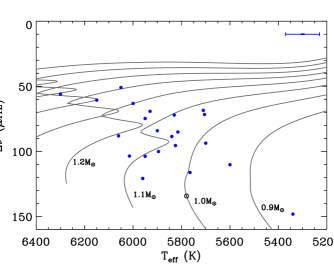
From the peak bagging results, we estimated the frequency of maximum power, $\nu_{\rm max}$ , by fitting a Gaussian to the extracted radial mode amplitudes as a function of frequency. We then took the 4 radial orders³³3The choice of the number of radial orders is a trade-off between reducing the error bar (large number of modes) and restricting the frequency range of the calculation to reduce the contribution of the frequency variation of $\Delta\nu$ . Using 4 orders was appropriate given the variation in $\langle\Delta\nu\rangle$ observed in the stars of our sample. closest to $\nu_{\rm max}$ to perform a weighted linear regression as a function of the order $n$ to compute the mean large frequency separation, $\langle\Delta\nu\rangle$ . Figure 1 presents a modified H-R diagram, where we substitute $\langle\Delta\nu\rangle$ as a proxy for the luminosity and use the effective temperature obtained from the spectroscopic analysis described in §2.2. Note that most of the stars selected for our analysis are hotter and more luminous than the Sun.

2.2. Non-seismic constraints

The atmospheric parameters $T_{\rm eff}$ , $\log g$ , and [Fe/H] were determined by analyzing high-quality spectra acquired from two service observing programs during the summer of 2010 (Bruntt et al., 2011) using the ESPADONs spectrograph at the Canada-France-Hawaii Telescope and the NARVAL spectrograph at the Bernard Lyot telescope. The spectra have a resolution of 80,000 and a typical signal-to-noise ratio in the continuum of 200-300. We employed the Versatile Wavelength Analysis (VWA) technique (Bruntt et al., 2010a, b) in which several hundred individual lines are iteratively fit by calculating synthetic profiles. We verified that our derived $T_{\rm eff}$ values agreed with the photometric calibration using the $V_{T}-K$ index (Casagrande et al., 2010). Uncertainties on the parameters $T_{\rm eff}$ , $\log g$ , and [Fe/H] are typically 70 K, 0.08 dex, and 0.07 dex, respectively, including statistical and systematic errors combined in quadrature. The values we used were the preliminary results of the spectroscopic analysis presented by Bruntt et al. (2011) but agree with the final results within the uncertainties. We did not have spectroscopic data for KIC 10018963 and KIC 11713510, so we used the $T_{\rm eff}$ values from Pinsonneault et al. (2011). To be sure that this does not introduce any bias in our analysis, for $\sim$ 15 stars we checked that the $T_{\rm eff}$ from the two methods agree within the error bars. For KIC 10018963 we also adopted the [Fe/H] value from the Kepler Input Catalog (KIC; Brown et al., 2011), but for KIC 11713510, we did not impose a constraint on [Fe/H]. For seven stars, we also had constraints on the luminosity via the parallaxes from van Leeuwen (2007a, b), and the Johnson $V$ and galactic extinction $E(B-V)$ from the Tycho catalog (Ammons et al., 2006). We applied the bolometric correction of Flower (1996) as tabulated in Torres (2010), adopting a solar bolometric absolute magnitude $M_{\rm bol,\odot}\,=\,4.73\pm 0.03$ to ensure internal consistency. All of the non-seismic constraints adopted for the stellar modeling are listed in Table 2.1, along with the corresponding properties of the optimal models from AMP (marked with an asterisk, see §4) and the value of the normalized $\chi^{2}_{\rm spec}$ from Eq. (5).

3. STELLAR MODELING METHODS

Four teams modeled the 22 stars using different methods. Three of the methods (RADIUS, YB, and SEEK) used model grids to fit the global oscillation properties, yielding the asteroseismic radius, mass, and age. One method (AMP) fit the individual oscillation frequencies to provide additional information such as the composition and mixing-length for each star. Below we describe the details of these four model-fitting methods.

3.1. RADIUS

The RADIUS method (Stello et al., 2009b) uses $T_{\rm eff}$ , $\log g$ , [Fe/H], $L$ , and $\langle\Delta\nu\rangle$ to find the optimal model. The method is based on a large grid of Aarhus STellar Evolution Code (ASTEC; Christensen-Dalsgaard, 2008a) models using the EFF equation of state (Eggleton et al., 1973). It uses the opacity tables of Rogers & Iglesias (1995) and Kurucz (1991) for $T<10^{4}$ K with the solar mixture of Grevesse & Noels (1993). Rotation, overshooting, and diffusion were not included. The grid was created with fixed values of the mixing-length parameter ( $\alpha=1.8$ ) and the initial hydrogen mass fraction ( $X_{\mathrm{i}}$ = 0.7). The resolution in $\log\,Z$ was 0.1 dex with $0.001<Z<0.055$ , and the resolution in mass was 0.01 $M_{\odot}$ from 0.5 to 4.0 $M_{\odot}$ . The evolution begins at the ZAMS and continues to the tip of the red-giant branch. To convert between the model values of $Z$ and the observed [Fe/H], we used $Z_{\odot}=0.0188$ (Cox, 2000). We made slight modifications to the RADIUS approach described by Stello et al. (2009b). First, the mean large frequency separation was derived by applying the scaling relations based on solar values (Kjeldsen & Bedding, 1995) instead of calculating it directly from the model frequencies. Although there is a known systematic difference between these two ways of deriving $\langle\Delta\nu\rangle$ , the effect is at the 1% level (Stello et al., 2009a; Basu et al., 2010; White et al., 2011a). Second, for each star, we pinpointed a single optimal model based on a $\chi^{2}$ formalism that was applied to all models within $\pm\,$ 3 $\sigma$ of the observational constraints. The uncertainties were computed as described by Stello et al. (2009b) based on the smallest and largest values of each parameter among the selected stellar models.

3.2. YB

The YB method uses a variant of the Yale-Birmingham code (Basu et al., 2010), as described by Gai et al. (2011). The method finds the maximum likelihood of the stellar radius, mass, and age from several grids of models using the values of $\langle\Delta\nu\rangle$ , $\nu_{\rm max}$ , $T_{\rm eff}$ and [Fe/H] as input. For each set of observational constraints, YB generates 10,000 new sets by adding different realizations of random Gaussian noise to the observed values. It then evaluates a likelihood function for each model in every grid:

\mathcal{L}=\left(\prod^{N}_{i=1}\frac{1}{\sqrt{2\pi}\sigma_{i}}\right)\times\exp(-\chi^{2}/2),

(1)

where

\chi^{2}=\sum^{N}_{i=1}\left(\frac{q_{{\rm obs},i}-q_{{\rm mod},i}}{\sigma_{i}}\right)^{2},

(2)

with $q\equiv$ { $\langle\Delta\nu\rangle$ , $\nu_{\rm max}$ , $T_{\rm eff}$ , [Fe/H]}, $N$ is the number observables and the $\sigma_{i}$ are the uncertainties on the observational constraints. The oscillation properties ( $\langle\Delta\nu\rangle$ and $\nu_{\rm max}$ ) of the models are derived from scaling relations (Kjeldsen & Bedding, 1995). All points from the 10,000 sets of constraints with $\mathcal{L}$ greater than 95% of the maximum likelihood form a distribution function for each stellar property, with the median indicating the estimated value and the 1 $\sigma$ limits providing a measure of the errors.

This method uses four different model grids for determining the properties of each star, which were derived from the Yale Rotating Evolution Code (YREC; Demarque et al., 2008) in its non-rotating configuration with up-to-date physics (for details, see Gai et al., 2011), the Yonsei-Yale isochrones (Demarque et al., 2004), the Dartmouth Stellar Evolution Database (Dotter et al., 2008), and the Padova code (Marigo et al., 2008). Each grid produced a set of results for each star, and the final result was taken to be the median of the results returned by the different grids with an additional contribution to the uncertainty from the dispersion in the individual results.

3.3. SEEK

The SEEK method uses a large grid of stellar models computed with ASTEC. The models in the grid were constructed using the OPAL equation of state (Rogers & Nayfonov, 2002), OPAL opacity tables (Iglesias & Rogers, 1996) augmented at low temperatures by Alexander & Ferguson (1994), and the solar mixture of Grevesse & Sauval (1998). The treatment of convection is based on mixing-length theory (Böhm-Vitense, 1958) with the convection efficiency parameter $\alpha$ . Diffusion and overshooting were not included. The grid consists of 7300 evolution tracks that are divided into 100 subsets with different combinations of metallicity ( $Z$ ), initial hydrogen mass fraction ( $X_{\mathrm{i}}$ ), and $\alpha$ , where: $0.0075\leq Z\leq 0.03$ and $0.68\leq X_{\mathrm{i}}\leq 0.74$ , and $0.8\leq\alpha\leq 2.8$ . To identify the best model, SEEK compares the observational constraints with every model in the grid and makes a Bayesian assessment of the uncertainties. The oscillation properties of the models are derived by computing the individual frequencies with the Aarhus adiabatic pulsation code (ADIPLS; Christensen-Dalsgaard, 2008b). Note that, unlike RADIUS and YB, the SEEK method includes the small separation ( $\delta_{02}$ ) as a constraint. Complete details of the method are provided in Quirion et al. (2010).

3.4. AMP

The Asteroseismic Modeling Portal (AMP) is the only method that attempts to fit the individual oscillation frequencies. This method is based on ASTEC models and the ADIPLS code, and it uses a parallel genetic algorithm (GA; Metcalfe & Charbonneau, 2003) to optimize the match between the model output and the observational constraints. The evolution code uses the OPAL 2005 equation of state (Rogers & Nayfonov, 2002) with the most recent OPAL opacities (Iglesias & Rogers, 1996) supplemented by Alexander & Ferguson (1994) opacities at low temperatures. Convection is treated with the mixing-length theory (Böhm-Vitense, 1958), and diffusion and gravitational settling of helium is included following the prescription of Michaud & Proffitt (1993). The GA searches a broad range of model parameters, including the mass from 0.75 to 1.75 M_⊙, the metallicity ( $Z$ ) from 0.002 to 0.050, the initial helium mass fraction ( $Y_{\mathrm{i}}$ ) from 0.22 to 0.32, and the mixing-length parameter ( $\alpha$ ) from 1 to 3. The stellar age is optimized internally for each model by matching the observed value of $\langle\Delta\nu_{0}\rangle$ using a binary decision tree (for details, see Metcalfe et al., 2009). While the methods presented above are based on grids of models that have been computed just once, AMP generates around $10^{5}$ models for each star.

An empirical correction for surface effects ( $a_{\nu}$ ) was applied to the model frequencies ( $\nu_{\rm mod}$ ) following Kjeldsen et al. (2008) before comparing the corrected frequencies ( $\nu_{\rm corr}$ ) with observations. The correction for each model frequency was calculated from:

a_{\nu}\equiv\nu_{\rm corr}-\nu_{\rm mod}=a_{0}\left(\frac{\nu_{\rm mod}}{\nu_{\rm max}}\right)^{b},

(3)

where $a_{0}$ is the size of the correction at $\nu_{\rm max}$ and the exponent was fixed to a solar calibrated value of $b=4.823$ . The value of $a_{0}$ for each model is determined from Kjeldsen et al. (2008, their Eq. (10)). To quantify the differences between each model and the observations, we calculate a normalized $\chi^{2}$ separately for the asteroseismic and the spectroscopic constraints:

\chi^{2}_{\rm seis}=\frac{1}{N_{\rm f}}\sum_{i=1}^{N_{\rm f}}\left(\frac{\nu_{{\rm obs},i}-\nu_{{\rm corr},i}}{\sigma_{{\rm obs},i}}\right)^{2}

(4)

and

\chi^{2}_{\rm spec}=\frac{1}{N_{\rm s}}\sum_{i=1}^{N_{\rm s}}\left(\frac{P_{{\rm obs},i}-P_{{\rm mod},i}}{\sigma_{{\rm obs},i}}\right)^{2},

(5)

where $\nu_{{\rm obs},i}$ are the $N_{\rm f}$ observed frequencies with corresponding uncertainties $\sigma_{{\rm obs},i}$ , and $\nu_{{\rm corr},i}$ are the model frequencies from AMP after applying the empirical surface correction. The $P_{{\rm obs},i}$ are the $N_{\rm s}$ non-seismic constraints ( $T_{\rm eff}$ , $\log g$ , [Fe/H], $L$ ), while $P_{{\rm mod},i}$ are the values of the corresponding observables from the optimal model. AMP minimizes the mean of the two $\chi^{2}$ values, and the uncertainties on the adjustable model parameters are determined using singular value decomposition (SVD).

The AMP pipeline is available through a TeraGrid Science Gateway (Woitaszek et al., 2009). AMP consists of two components: a web-based user interface that supports submitting new jobs and viewing existing results, and a back-end workflow automation engine (called GridAMP) that manages the execution of the underlying science codes on Grid-enabled clusters and supercomputers such as those on the TeraGrid (Hazlewood & Woitaszek, 2011). The AMP Science Gateway greatly simplifies the use of the pipeline by automating the many calls of the Fortran code that are required to propagate the genetic algorithms to completion; it also prepares initial échelle and H-R diagrams for inspection, notifies the user when the processing is complete, and archives the results with appropriate catalog cross-references for later comparison.

4. RESULTS

For many purposes, the most interesting quantities to emerge from asteroseismology are the radius, mass, and age of the star. In the case of an exoplanet host star, the stellar radius is needed to establish the absolute planetary radius from transit photometry. The mass provides the absolute scale of the orbit and when combined with radial velocity measurements can lead to an estimate of the mass of the planet. The age is important for assessing the dynamical stability of the system and establishing its chronology with respect to other planetary systems. There are several levels of asteroseismic analysis that can provide some of these quantities, and all of them need to be exploited to provide as much information as possible for a wide range of Kepler targets.

For the faintest targets, where only the global oscillation properties ( $\langle\Delta\nu\rangle$ , $\nu_{\rm max}$ ) can be determined from the data, empirical scaling relations can be used in conjunction with an inferred $T_{\rm eff}$ to estimate the stellar radius and mass. Model-grid-based methods can use additional information from spectroscopy ( $\log g$ , [Fe/H]) to provide more precise estimates of the radius and mass, along with some information about the stellar age. The most precise constraints on all of these properties—as well as information about the stellar composition and mixing-length—come from fitting the individual oscillation frequencies, which can only be extracted for the best and brightest targets. In this section we describe the results of applying all of these analysis methods to our sample of 22 stars, allowing us to quantify the relative precision of these techniques. The results from AMP are expected to be the most precise, so we use them as the reference when evaluating the other methods and we define and quantify the systematic uncertainties as the offsets from the AMP results, hereafter called relative accuracy.

4.1. Scaling relations

The empirical scaling relations of Kjeldsen & Bedding (1995) can be used to provide first estimates of the stellar radius and mass without any stellar modeling:

\frac{R}{R_{\odot}}\,\approx\,\left(\frac{135~{}\mu{\rm Hz}}{\langle\Delta\nu\rangle}\right)^{2}\left(\frac{\nu_{\rm max}}{3050~{}\mu{\rm Hz}}\right)\left(\frac{T_{\rm eff}}{5777~{}{\rm K}}\right)^{1/2}\\

(6)

\frac{M}{M_{\odot}}\,\approx\,\left(\frac{135~{}\mu{\rm Hz}}{\langle\Delta\nu\rangle}\right)^{4}\left(\frac{\nu_{\rm max}}{3050~{}\mu{\rm Hz}}\right)^{3}\left(\frac{T_{\rm eff}}{5777~{}{\rm K}}\right)^{3/2}\\

(7)

where $\langle\Delta\nu\rangle$ is the observed mean large frequency separation, $\nu_{\rm max}$ is the observed frequency of maximum power, and $T_{\rm eff}$ is the effective temperature. These relations have recently been tested for solar-type stars and red giants (Huber et al., 2010) and overall they appear to be in good agreement with the observations. The median statistical uncertainties from our sample of 22 stars suggest that these scaling relations typically provide a radius precision of 3% and a mass precision of 9%.

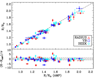
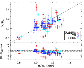
In Figure 2, we compare the values of the radius and mass estimated from these scaling relations with the results obtained from AMP (see §4.3). In the top of each panel we plot the actual values from each method, while in the bottom we show the differences between the methods in units of the statistical uncertainty, $\sigma$ , computed as the quadratic sum of the uncertainties from the two methods being compared. The stellar radii from the two methods are in very good agreement, suggesting that observations of the global oscillation properties combined with an effective temperature can provide reliable estimates of the radius, though with lower precision than when using stellar models to fit the individual frequencies (0.8%, see §4.3). The exponents on the scaling relations for the stellar mass are a factor of 2–3 higher on each observable compared to the scaling relations for the radius, so we expect a larger scatter. Even so, the agreement between methods is good. The scaling relations tend to overestimate the radius by $+\,0.3\,\sigma$ and the mass by $+\,0.4\,\sigma$ relative to the values from AMP, where $\sigma$ depends on the uncertainties given by the scaling relations. The largest deviations are found for subgiants that exhibit mixed modes (KIC 5512589, 7976303, 8228742, 10018963, 11244118), suggesting that the measurement of $\langle\Delta\nu\rangle$ and $\nu_{\rm max}$ with our method can be slightly biased in such cases or that the scaling relations may be less reliable for these stars.

Table 1Global oscillation properties from 1 month of data and model-grid-based results^a^afootnotemark:

KIC	Quarter	$\nu_{\rm max}$ ( $\mu$ Hz)	$\langle\Delta\nu\rangle$ ( $\mu$ Hz)	Method	$R~{}(R_{\odot})$	$M~{}(M_{\odot})$	$t$ (Gyr)
3632418	Q2.3	$1110\pm 20$	$60.63\pm 0.37$	RADIUS	$1.80\pm 0.02$	$1.19\pm 0.04$	$4.20\pm 0.58$
				YB	1.83 ${}^{+0.03}_{-0.05}$	1.22 ${}^{+0.04}_{-0.06}$	4.65 ${}^{+0.88}_{-0.61}$
				SEEK	1.83 ${}^{+0.04}_{-0.03}$	1.28 ${}^{+0.10}_{-0.06}$	2.67 ${}^{+0.42}_{-0.41}$
3656476	Q1	$1940\pm 25$	$93.70\pm 0.22$	RADIUS	$1.38\pm 0.02$	$1.29\pm 0.06$	$5.04\pm 1.56$
				YB	$1.28\pm 0.02$	$1.05\pm 0.04$	8.85 ${}^{+1.62}_{-3.21}$
				SEEK	$1.32\pm 0.02$	1.05 ${}^{+0.06}_{-0.03}$	9.87 ${}^{+1.74}_{-0.96}$
4914923	Q1	$1835\pm 60$	$88.61\pm 0.32$	RADIUS	$1.40\pm 0.02$	$1.21\pm 0.05$	$5.04\pm 1.44$
				YB	1.37 ${}^{+0.02}_{-0.04}$	$1.12\pm 0.05$	6.59 ${}^{+1.30}_{-1.81}$
				SEEK	1.42 ${}^{+0.02}_{-0.04}$	1.20 ${}^{+0.06}_{-0.09}$	4.83 ${}^{+1.43}_{-0.75}$
5184732	Q2.2	$2070\pm 20$	$95.53\pm 0.26$	RADIUS	$1.38\pm 0.02$	$1.33\pm 0.05$	$3.57\pm 1.14$
				YB	$1.31\pm 0.02$	$1.15\pm 0.07$	5.27 ${}^{+1.92}_{-1.61}$
				SEEK	$1.33\pm 0.02$	1.16 ${}^{+0.06}_{-0.02}$	5.07 ${}^{+0.76}_{-0.53}$
5512589	Q2.3	$1240\pm 25$	$68.52\pm 0.33$	RADIUS	$1.60\pm 0.02$	$1.08\pm 0.04$	$8.76\pm 1.14$
				YB	1.60 ${}^{+0.02}_{-0.03}$	1.05 ${}^{+0.04}_{-0.03}$	8.83 ${}^{+1.18}_{-1.88}$
				SEEK	1.64 ${}^{+0.04}_{-0.03}$	1.11 ${}^{+0.12}_{-0.08}$	8.75 ${}^{+1.21}_{-5.19}$
6106415	Q2.2	$2285\pm 20$	$103.82\pm 0.29$	RADIUS	$1.21\pm 0.01$	$1.07\pm 0.03$	$5.11\pm 0.80$
				YB	1.24 ${}^{+0.02}_{-0.01}$	1.10 ${}^{+0.04}_{-0.03}$	4.96 ${}^{+1.20}_{-0.92}$
				SEEK	$1.33\pm 0.03$	1.16 ${}^{+0.06}_{-0.10}$	5.07 ${}^{+0.50}_{-0.45}$
6116048	Q2.2	$2120\pm 20$	$100.14\pm 0.22$	RADIUS	$1.16\pm 0.01$	$0.86\pm 0.03$	$11.54\pm 1.18$
				YB	1.24 ${}^{+0.01}_{-0.02}$	$1.03\pm 0.03$	7.23 ${}^{+1.36}_{-1.38}$
				SEEK	1.19 ${}^{+0.04}_{-0.03}$	0.93 ${}^{+0.07}_{-0.05}$	7.02 ${}^{+1.84}_{-1.42}$
6603624	Q1	$2405\pm 50$	$110.28\pm 0.25$	RADIUS	$1.18\pm 0.02$	$1.10\pm 0.04$	$8.23\pm 1.67$
				YB	$1.13\pm 0.01$	1.01 ${}^{+0.06}_{-0.04}$	8.62 ${}^{+1.82}_{-1.55}$
				SEEK	$1.18\pm 0.02$	1.09 ${}^{+0.04}_{-0.06}$	7.71 ${}^{+0.57}_{-0.26}$
6933899	Q2.1	$1370\pm 30$	$72.15\pm 0.25$	RADIUS	$1.59\pm 0.02$	$1.15\pm 0.04$	$6.31\pm 1.13$
				YB	$1.57\pm 0.02$	$1.10\pm 0.04$	7.08 ${}^{+1.66}_{-1.11}$
				SEEK	$1.60\pm 0.03$	1.15 ${}^{+0.09}_{-0.05}$	5.40 ${}^{+1.71}_{-1.81}$
7680114	Q2.3	$1660\pm 25$	$85.13\pm 0.14$	RADIUS	$1.39\pm 0.02$	$1.08\pm 0.05$	$7.80\pm 1.53$
				YB	1.35 ${}^{+0.03}_{-0.02}$	1.03 ${}^{+0.04}_{-0.03}$	8.91 ${}^{+1.91}_{-1.10}$
				SEEK	1.44 ${}^{+0.02}_{-0.03}$	1.17 ${}^{+0.07}_{-0.05}$	6.93 ${}^{+2.21}_{-3.99}$
7976303	Q1	$910\pm 25$	$50.95\pm 0.37$	RADIUS	$1.93\pm 0.02$	$1.04\pm 0.03$	$5.57\pm 0.61$
				YB	2.07 ${}^{+0.05}_{-0.07}$	1.10 ${}^{+0.05}_{-0.08}$	5.65 ${}^{+1.35}_{-0.45}$
				SEEK	1.98 ${}^{+0.03}_{-0.05}$	1.05 ${}^{+0.08}_{-0.04}$	5.00 ${}^{+0.93}_{-0.62}$
8006161	Q2.2	$3545\pm 140$	$148.21\pm 0.19$	RADIUS	$0.96\pm 0.01$	$1.07\pm 0.03$	$4.44\pm 1.73$
				YB	$0.91\pm 0.01$	0.96 ${}^{+0.08}_{-0.04}$	5.06 ${}^{+2.11}_{-2.35}$
				SEEK	$0.93\pm 0.02$	$1.00\pm 0.02$	5.46 ${}^{+0.30}_{-0.84}$
8228742	Q1	$1160\pm 40$	$63.15\pm 0.32$	RADIUS	$1.70\pm 0.02$	$1.08\pm 0.04$	$6.50\pm 0.72$
				YB	1.75 ${}^{+0.05}_{-0.06}$	1.18 ${}^{+0.05}_{-0.06}$	5.52 ${}^{+1.01}_{-0.95}$
				SEEK	1.73 ${}^{+0.05}_{-0.02}$	1.17 ${}^{+0.05}_{-0.02}$	2.77 ${}^{+1.58}_{-0.10}$
8379927	Q2.1	$2880\pm 65$	$120.86\pm 0.43$	RADIUS	$1.01\pm 0.01$	$0.84\pm 0.03$	$11.21\pm 1.24$
				YB	$1.13\pm 0.02$	$1.10\pm 0.06$	3.22 ${}^{+2.00}_{-1.69}$
				SEEK	$1.06\pm 0.03$	0.98 ${}^{+0.05}_{-0.08}$	4.71 ${}^{+0.93}_{-0.85}$
8760414	Q1	$2510\pm 95$	$116.24\pm 0.56$	RADIUS	$1.01\pm 0.01$	$0.78\pm 0.01$	$13.64\pm 0.22$
				YB	1.04 ${}^{+0.02}_{-0.01}$	0.82 ${}^{+0.01}_{-0.01}$	12.60 ${}^{+0.67}_{-0.01}$
				SEEK	$1.03\pm 0.02$	$0.83\pm 0.02$	$11.90\pm 0.10$
10018963	Q2.3	$985\pm 10$	$55.99\pm 0.35$	RADIUS	$1.81\pm 0.07$	$1.04\pm 0.12$	$5.13\pm 1.22$
				YB	1.90 ${}^{+0.06}_{-0.03}$	1.18 ${}^{+0.09}_{-0.06}$	4.65 ${}^{+0.39}_{-0.80}$
				SEEK	1.93 ${}^{+0.10}_{-0.08}$	1.24 ${}^{+0.21}_{-0.14}$	3.69 ${}^{+0.87}_{-1.53}$
10516096	Q1	$1710\pm 15$	$84.15\pm 0.36$	RADIUS	$1.36\pm 0.03$	$1.00\pm 0.05$	$8.13\pm 1.52$
				YB	$1.18\pm 0.03$	$1.02\pm 0.04$	7.77 ${}^{+1.33}_{-1.59}$
				SEEK	$1.41\pm 0.03$	1.05 ${}^{+0.10}_{-0.05}$	7.36 ${}^{+1.74}_{-2.04}$
10963065	Q2.3	$2160\pm 35$	$103.61\pm 0.41$	RADIUS	$1.17\pm 0.02$	$0.95\pm 0.04$	$7.62\pm 1.54$
				YB	$1.19\pm 0.03$	1.02 ${}^{+0.06}_{-0.07}$	7.07 ${}^{+1.64}_{-1.95}$
				SEEK	$1.21\pm 0.02$	1.03 ${}^{+0.07}_{-0.05}$	4.99 ${}^{+1.26}_{-0.77}$
11244118	Q2.1	$1405\pm 20$	$71.68\pm 0.16$	RADIUS	$1.71\pm 0.03$	$1.44\pm 0.07$	$3.95\pm 1.21$
				YB	1.57 ${}^{+0.03}_{-0.02}$	1.14 ${}^{+0.05}_{-0.06}$	7.50 ${}^{+1.08}_{-1.18}$
				SEEK	$1.63\pm 0.02$	$1.29\pm 0.02$	1.79 ${}^{+0.10}_{-0.13}$
11713510	Q1	$1235\pm 15$	$69.22\pm 0.20$	RADIUS	$\cdots$	$\cdots$	$\cdots$
				YB	$\cdots$	$\cdots$	$\cdots$
				SEEK	$1.60\pm 0.06$	1.04 ${}^{+0.14}_{-0.07}$	7.33 ${}^{+1.14}_{-1.47}$
12009504	Q1	$1825\pm 20$	$88.10\pm 0.42$	RADIUS	$1.34\pm 0.02$	$1.03\pm 0.05$	$6.77\pm 1.15$
				YB	$1.39\pm 0.02$	1.14 ${}^{+0.04}_{-0.03}$	5.02 ${}^{+0.97}_{-0.64}$
				SEEK	$1.40\pm 0.03$	1.18 ${}^{+0.08}_{-0.03}$	1.40 ${}^{+1.07}_{-0.47}$
12258514	Q1	$1475\pm 30$	$74.75\pm 0.23$	RADIUS	$1.56\pm 0.03$	$1.17\pm 0.05$	$5.62\pm 1.12$
				YB	1.55 ${}^{+0.03}_{-0.04}$	$1.16\pm 0.06$	$5.91\pm 1.31$
				SEEK	$1.65\pm 0.02$	1.37 ${}^{+0.03}_{-0.04}$	2.30 ${}^{+0.24}_{-0.10}$

4.2. Model-grid-based results

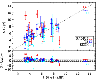
The three model-grid-based methods yielded estimates of the radius, mass, and age for most of the stars in our sample, except for one case where [Fe/H] was not available. These results are listed in Table 1, along with the global oscillation properties that were used as observational constraints. In Figure 3 we compare all of these results to the values obtained by AMP, again comparing the actual values and the differences in units of the statistical uncertainty, $\sigma$ , computed as the quadratic sum of the uncertainties from the two methods being compared. The horizontal coordinates for YB and SEEK have been shifted slightly to the left and to the right respectively (by $\pm$ 0.02 $R_{\odot}$ , $\pm$ 0.02 $M_{\odot}$ and $\pm$ 0.1 Gyr) to prevent the points from different methods overlapping.

The top panel of Figure 3 shows that the different results for the radius agree quite well. By using additional information from spectroscopy, these methods generally improve upon the precision that is possible from empirical scaling relations. The median statistical uncertainties on the radius are 1.4% for RADIUS, ${}^{+\,3.0\%}_{-\,1.6\%}$ for YB, and ${}^{+\,4.9\%}_{-\,2.1\%}$ for SEEK. Although there are some outliers, the absolute level of agreement between the various methods is also quite encouraging. The mean systematic offsets (or relative accuracy) for each of the methods relative to AMP are $-\,1.4\,\sigma$ for RADIUS, $-\,1.2\,\sigma$ for YB and $+\,0.01\,\sigma$ for SEEK, implying a general tendency for the model-grid-based methods to slightly underestimate the stellar radius. These differences are related to the method used to find the best fit and to the different physics included in the stellar models. Note that SEEK and AMP use very similar input physics (See § 3.4).

The middle panel of Figure 3 shows a larger dispersion in the values of the mass derived from model-grid-based methods compared to the radius, but the overall agreement is still reasonable. The three methods all yield a median mass precision in the range 4–6%, again providing some improvement over empirical scaling relations. There is some indication of a mass-dependent systematic error in the results from model-grid-based methods compared to the values obtained with AMP, with the former more severely underestimating the mass at higher masses. However, the relative accuracy is still reasonable with mean systematic offset relative to AMP of $-1.5\,\sigma$ for RADIUS, $-1\,\sigma$ for YB and $-0.2\,\sigma$ for SEEK. Most of the stars that show significant disagreement between the values of the radius and mass derived from model-grid-based methods and those derived from fitting the individual frequencies with AMP are evolved stars with mixed modes. This underscores the potential for slight biases in the analysis of such targets when fitting only the global oscillation properties with stellar models. The larger systematic offsets in radius and mass for the grid-based methods compared to the scaling relations, in terms of $\sigma$ , is related to the fact that $\sigma$ depends on the internal uncertainties.

Finally, the bottom panel of Figure 3 compares the stellar ages estimated by the different methods. The scatter in the derived values is even larger than for the mass, but when the differences are normalized by the quoted uncertainties the overall agreement looks more reasonable. The median age precision from the model-grid-based methods ranges from 15 to 21%, and the mean offset relative to AMP is $+1.5\,\sigma$ for RADIUS, $+0.8\,\sigma$ for YB and $-0.2\,\sigma$ for SEEK. Once again there is some indication of a trend in the systematic errors, with the model-grid-based methods more seriously overestimating the age for the youngest stars. For main sequence stars, the small separation provides the strongest constraint on the age in the absence of fitting the individual frequencies (White et al., 2011a). However, not all of the model-grid-based methods include the small separation as a constraint. This is the case for RADIUS, which exhibits the largest mean systematic offset in the ages compared to AMP. Only one of the four grids employed by the YB method tabulates the small separation, so this method is known to provide less reliable ages for single stars (Gai et al., 2011). SEEK is the only method that fully incorporates the observed small separation in the fitting, yielding ages that are most consistent with AMP.

4.3. AMP results

The most precise results for the radius, mass, and age came from using AMP to fit the individual oscillation frequencies, along with the spectroscopic and other observational constraints (see §2). The empirical correction for surface effects and the corrected model frequencies are tabulated in Appendix A (available in the online material) with the observed frequencies for each target. An example is shown in Table 2.1, where we include the model frequencies for several radial orders above and below the range of observed modes to facilitate the identification of newly detected modes in the longer data sets that are expected for these stars in the future.

Table 2Properties of the optimal models and surface correction from AMP results¹¹For each star, we give the radius (

R

), the mass (

M

), the age (

t

), the metallicity (

Z

), the initial He mass fraction (

Y_{i}

), the mixing-length parameter (

\alpha

), position of the base of the convection zone (

r_{\rm CZ}

), and the size of the surface correction at

\nu_{\rm max}

(

a_{0}

) in

\mu

Hz for the optimal model from AMP. The normalized

\chi^{2}_{\rm seis}

is calculated from Eq. (4). Quoted errors include only the statistical uncertainties. See §4 for a discussion of the systematics.

KIC	$R~{}(R_{\odot})$	$M~{}(M_{\odot})$	$t$ (Gyr)	$Z$	$Y_{\rm i}$	$\alpha$	$r_{\rm CZ}(R)$	$a_{0}$	$\chi_{\rm seis}^{2}$
3632418	1.84 $\pm$ 0.01	1.28 $\pm$ 0.01	3.16 $\pm$ 0.05	0.0121 $\pm$ 0.0001	0.256 $\pm$ 0.002	1.68 $\pm$ 0.02	0.851 ${}^{+0.003}_{-0.002}$	$-$ 1.96	5.9
3656476	1.32 $\pm$ 0.03	1.09 $\pm$ 0.01	7.71 $\pm$ 0.22	0.0309 $\pm$ 0.0024	0.278 $\pm$ 0.001	1.96 $\pm$ 0.06	0.677 ${}^{+0.006}_{-0.010}$	$-$ 4.87	3.2
4914923	1.37 $\pm$ 0.05	1.10 $\pm$ 0.01	6.18 $\pm$ 0.18	0.0203 $\pm$ 0.0020	0.267 $\pm$ 0.001	1.90 $\pm$ 0.07	0.725 ${}^{+0.013}_{-0.025}$	$-$ 4.91	6.1
5184732	1.36 $\pm$ 0.01	1.25 $\pm$ 0.01	3.98 $\pm$ 0.11	0.0413 $\pm$ 0.0026	0.280 $\pm$ 0.007	1.96 $\pm$ 0.08	0.728 ${}^{+0.007}_{-0.007}$	$-$ 3.92	7.2
5512589	1.67 $\pm$ 0.01	1.16 $\pm$ 0.01	7.68 $\pm$ 0.04	0.0203 $\pm$ 0.0004	0.234 $\pm$ 0.001	1.86 $\pm$ 0.02	0.728 ${}^{+0.010}_{-0.010}$	$-$ 2.57	4.7
6106415	1.24 $\pm$ 0.01	1.12 $\pm$ 0.02	4.72 $\pm$ 0.12	0.0173 $\pm$ 0.0014	0.246 $\pm$ 0.013	2.00 $\pm$ 0.08	0.750 ${}^{+0.007}_{-0.005}$	$-$ 4.24	4.6
6116048	1.26 $\pm$ 0.01	1.12 $\pm$ 0.02	5.26 $\pm$ 0.13	0.0134 $\pm$ 0.0013	0.220 $\pm$ 0.017	1.94 $\pm$ 0.07	0.762 ${}^{+0.007}_{-0.010}$	$-$ 3.82	12.5
6603624	1.15 $\pm$ 0.01	1.01 $\pm$ 0.01	8.51 $\pm$ 0.23	0.0299 $\pm$ 0.0027	0.284 $\pm$ 0.010	1.84 $\pm$ 0.07	0.672 ${}^{+0.003}_{-0.003}$	$-$ 4.71	1.9
6933899	1.58 $\pm$ 0.01	1.10 $\pm$ 0.01	6.28 $\pm$ 0.15	0.0191 $\pm$ 0.0008	0.282 $\pm$ 0.001	1.98 $\pm$ 0.05	0.714 ${}^{+0.010}_{-0.010}$	$-$ 3.29	3.6
7680114	1.45 $\pm$ 0.03	1.19 $\pm$ 0.01	5.92 $\pm$ 0.20	0.0210 $\pm$ 0.0010	0.240 $\pm$ 0.013	2.00 $\pm$ 0.14	0.712 ${}^{+0.008}_{-0.009}$	$-$ 2.32	5.9
7976303	2.03 $\pm$ 0.05	1.17 $\pm$ 0.02	5.81 $\pm$ 0.03	0.0100 $\pm$ 0.0010	0.225 $\pm$ 0.001	1.66 $\pm$ 0.01	0.755 ${}^{+0.010}_{-0.010}$	$-$ 1.81	7.7
8006161	0.93 $\pm$ 0.00	1.00 $\pm$ 0.01	4.28 $\pm$ 0.12	0.0309 $\pm$ 0.0026	0.258 $\pm$ 0.015	1.84 $\pm$ 0.09	0.685 ${}^{+0.002}_{-0.003}$	$-$ 6.64	4.2
8228742	1.84 $\pm$ 0.01	1.31 $\pm$ 0.01	4.26 $\pm$ 0.02	0.0173 $\pm$ 0.0002	0.228 $\pm$ 0.001	1.76 $\pm$ 0.01	0.827 ${}^{+0.001}_{-0.001}$	$-$ 2.60	9.8
8379927	1.11 $\pm$ 0.02	1.09 $\pm$ 0.03	3.28 $\pm$ 0.16	0.0162 $\pm$ 0.0029	0.234 $\pm$ 0.032	1.66 $\pm$ 0.16	0.758 ${}^{+0.010}_{-0.018}$	$-$ 4.55	3.8
8760414	1.02 $\pm$ 0.01	0.81 $\pm$ 0.01	13.35 $\pm$ 0.38	0.0034 $\pm$ 0.0004	0.220 $\pm$ 0.018	1.82 $\pm$ 0.08	0.721 ${}^{+0.010}_{-0.012}$	$-$ 5.30	6.5
10018963	1.91 $\pm$ 0.01	1.17 $\pm$ 0.01	3.66 $\pm$ 0.02	0.0107 $\pm$ 0.0001	0.291 $\pm$ 0.001	2.12 $\pm$ 0.01	0.825 ${}^{+0.001}_{-0.001}$	$-$ 1.59	12.6
10516096	1.42 $\pm$ 0.03	1.12 $\pm$ 0.03	6.41 $\pm$ 0.27	0.0147 $\pm$ 0.0019	0.232 $\pm$ 0.022	1.88 $\pm$ 0.13	0.745 ${}^{+0.018}_{-0.018}$	$-$ 3.64	1.1
10963065	1.20 $\pm$ 0.09	1.03 $\pm$ 0.03	3.90 $\pm$ 0.04	0.0107 $\pm$ 0.0012	0.271 $\pm$ 0.020	1.66 $\pm$ 0.10	0.809 ${}^{+0.015}_{-0.015}$	$-$ 5.39	3.0
11244118	1.55 $\pm$ 0.01	1.01 $\pm$ 0.01	8.93 $\pm$ 0.04	0.0280 $\pm$ 0.0001	0.318 $\pm$ 0.002	2.16 $\pm$ 0.01	0.598 ${}^{+0.010}_{-0.010}$	$-$ 0.91	6.2
11713510	1.57 $\pm$ 0.01	1.00 $\pm$ 0.00	7.82 $\pm$ 0.04	0.0100 $\pm$ 0.0001	0.265 $\pm$ 0.001	2.10 $\pm$ 0.01	0.690 ${}^{+0.001}_{-0.010}$	$-$ 3.17	4.7
12009504	1.43 $\pm$ 0.04	1.26 $\pm$ 0.02	3.54 $\pm$ 0.12	0.0168 $\pm$ 0.0015	0.220 $\pm$ 0.007	1.86 $\pm$ 0.11	0.809 ${}^{+0.006}_{-0.017}$	$-$ 3.24	4.7
12258514	1.59 $\pm$ 0.01	1.22 $\pm$ 0.01	4.49 $\pm$ 0.09	0.0197 $\pm$ 0.0005	0.262 $\pm$ 0.004	1.78 $\pm$ 0.05	0.755 ${}^{+0.005}_{-0.004}$	$-$ 3.05	14.4

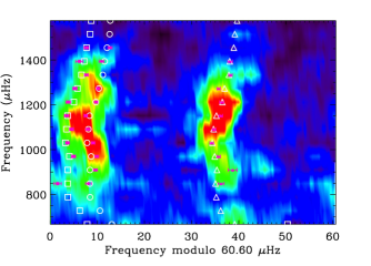
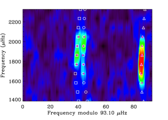
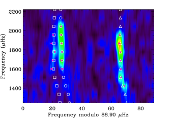
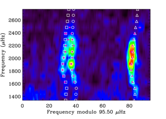
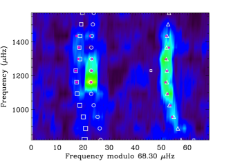
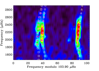
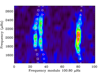
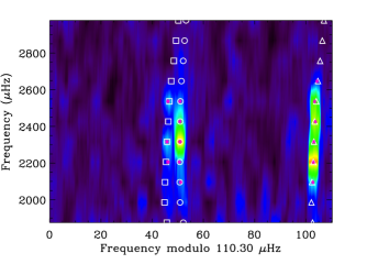
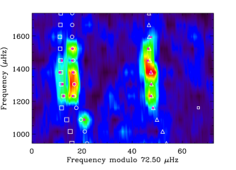
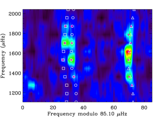
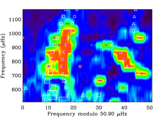
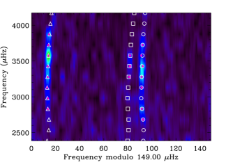
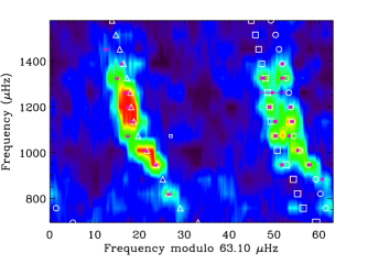
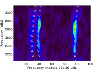
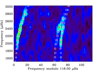
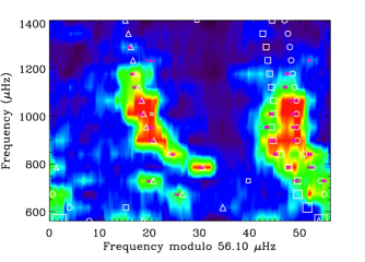
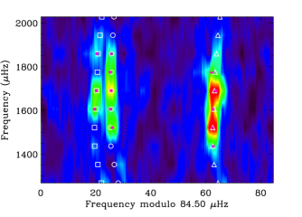
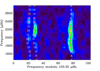
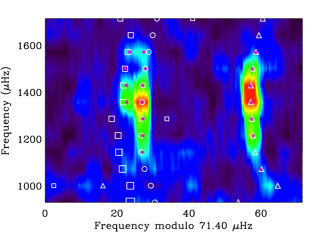
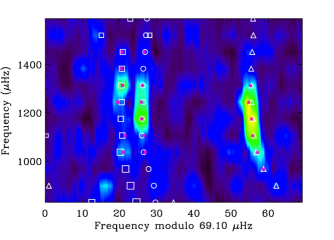
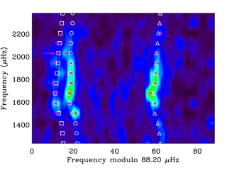
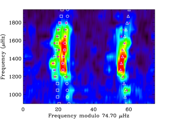
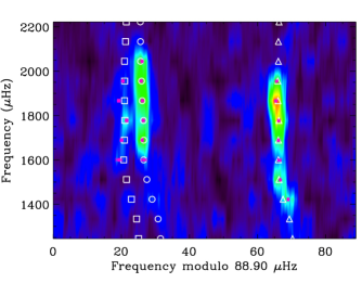
In Figure 4 we show a sample échelle diagram where the observed and model frequencies are compared graphically. In this representation of the data, we divide the oscillation spectrum into segments of length $\langle\Delta\nu\rangle$ and stack them so that modes with the same spherical degree are aligned almost vertically, with quadrupole ( $\ell=2$ ) and radial ( $\ell=0$ ) modes together on one side of the diagram and dipole ( $\ell=1$ ) modes on the other side. Against the background of the smoothed power spectrum, the observed frequencies are shown as solid pink symbols with error bars and the model frequencies are shown as open white symbols. Without the empirical correction for surface effects, the offset between the observations and the model at high frequencies would be up to $\sim$ 8 $\mu$ Hz, so incorporating this correction into our model-fitting procedure was essential to obtain a reasonable agreement. The example shown in Figure 4 is typical of the quality we obtained with AMP, and similar échelle diagrams are included in Appendix B (available in the online material) for each of the 22 stars in our sample.

The properties of the optimal models from AMP are listed in Table 2, including the values and statistical uncertainties of the adjustable model parameters ( $M,Z,Y_{\rm i},\alpha,t$ ), as well as the stellar radius, the magnitude of the surface correction at $\nu_{\rm max}$ ( $a_{0}$ ), an estimate of the model fractional radius at the base of the surface convection zone ( $r_{\rm CZ}$ ), and the value of the normalized $\chi^{2}_{\rm seis}$ from Eq. (4). The spectroscopic and other properties of the models obtained by AMP are listed in Table 2.1 with the corresponding observational constraints and the value of the normalized $\chi^{2}_{\rm spec}$ from Eq. (5). By fitting the individual oscillation frequencies instead of the global oscillation properties, we have further improved the precision on the radius, mass, and age. The median value of the internal uncertainties on the radius is 0.8%, a factor of two better than the best of the model-grid-based methods. For the mass AMP yields a median precision of 1.2%, a factor of five improvement over the model-grid-based results. Most significantly, the asteroseismic ages from AMP have a median statistical uncertainty of 2.5%, nearly an order of magnitude more precise than the model-grid-based methods. Indeed, the strongest constraints on the stellar age come from the observation of mixed modes in subgiants (Metcalfe et al., 2010; Deheuvels et al., 2010), where the age precision can be better than 1%.

The absolute accuracy of the derived stellar properties (i.e. the influence of possible systematic errors) is more difficult to assess than the internal precision. However, the level of agreement between the results from AMP and the empirical scaling relations and model-grid-based methods (see Figures 2 and 3) suggests that the systematic errors are comparable to the statistical uncertainties on the differences between various methods. The largest offsets from the AMP values for the radius, mass, and age were $\sim$ 1.5 $\,\sigma$ for the RADIUS method, which uses models with the simplified EFF equation of state. The smallest differences ( $\sim$ 0.2 $\,\sigma$ ) came from the SEEK method, which uses nearly the same models as AMP but without including diffusion and gravitational settling of helium. The uncertainties quoted by the YB method include a contribution from the dispersion of the results across four different model grids, and thus incorporate some systematics which typically agree with the AMP results at the $\sim$ 1 $\,\sigma$ level. Even so, we note that there may be additional uncertainties and errors in the modeling methods and physics, which could contribute to systematic errors on the inferred properties.

We attempted to quantify the possible systematic errors arising from our treatment of surface effects by modifying the weighting scheme that AMP uses when fitting the oscillation frequencies. The default scheme is to weight each frequency according to its statistical uncertainty. An alternative is to treat the empirical surface correction as a systematic error in the models (Guenther & Brown, 2004), and to combine half of this systematic in quadrature with the statistical uncertainty before determining the value of the normalized $\chi^{2}_{\rm seis}$ . The surface correction is calculated and applied just as before, but the weights of the highest frequencies are dramatically reduced and AMP is essentially biased towards fitting the low frequencies, where the surface correction is almost negligible. For unevolved stars in the asymptotic regime where the ridges in the échelle diagram are nearly vertical, models that fit well at lower frequencies will usually also fit the higher frequency modes. The alternate weighting scheme is not appropriate for stars that do not show asymptotic ridges (e.g. subgiants with mixed modes) because a fit to the low frequency modes will not generally lead to a reasonable match at higher frequencies. We repeated our fitting with AMP using this alternate weighting scheme for the subset of stars in our sample that showed clean vertical ridges in the échelle diagram (KIC 5184732, 6106415, 6116048, 6603624, 8006161, 10516096, 10963065). The mean offsets between the resulting sets of model parameters were $\Delta M\,=\,+\,0.01\,\ M_{\odot}$ , $\Delta t\,=\,-\,0.25$ Gyr, $\Delta Z\,=\,+\,0.0005$ , $\Delta Y_{\rm i}\,=\,+\,0.008$ , and $\Delta\alpha\,=\,-\,0.06$ suggesting that the changes are comparable to the mean uncertainties and our treatment of surface effects does not strongly bias the results. Note that the mean offsets may not be appropriate in every case and at best represent a fraction of the true systematic uncertainties, so we only include the statistical uncertainties in Table 2.

Fitting the individual frequencies gives AMP access to information that is not available from the global oscillation properties, so it can provide additional information such as the composition and mixing-length for the optimal models. The metallicity is primarily constrained by the spectroscopic [Fe/H], but it also has a strong influence on the stellar structure. If there is a conflict between the spectroscopic and asteroseismic constraints, the result will be an optimal model that does not satisfy either set of constraints very well. The two stars with the largest values of the normalized $\chi^{2}_{\rm spec}$ in Table 2.1 also have the lowest spectroscopic metallicities: KIC 7976303 with $[{\rm Fe/H}]=-0.52$ and KIC 8760414 with $[{\rm Fe/H}]=-1.19$ . In both cases AMP identified a reasonable match to the asteroseismic constraints (normalized $\chi^{2}_{\rm seis}\sim 7$ , see Table 2), but only by deviating significantly from the spectroscopic constraints. These problems could be related to the observed spectra, the abundance analysis or inadequacies in the stellar models underlying AMP.

Extreme values of the derived stellar properties are generally the sign of a problem with one or more of the observational constraints. In addition to the lowest metallicity, KIC 8760414 also has the lowest derived mass and the oldest inferred age in the sample, and it is one of several stars with an initial helium mass fraction well below the standard Big Bang nucleosynthesis value of $Y_{\rm i}=0.248$ (Spergel et al., 2007). We allowed AMP to search these low values of $Y_{\rm i}$ to allow for possible systematic errors, which is a common problem in stellar modeling (Casagrande et al., 2007; Troisi et al., 2011). Low values of $Y_{\rm i}$ are also found for KIC 8228742 (the highest derived mass) and KIC 7976303 (the largest radius and lowest mixing-length). The largest value of $Y_{\rm i}$ is found for KIC 11244118, which also has the highest mixing-length.

The radial extent of the convection zone ( $r_{\rm CZ}$ ) is important to characterize dynamo processes and to determine the surface amplitudes of gravity modes. The values of $r_{\rm CZ}$ listed in Table 2 are estimates from the optimal model of AMP, thus for a given physics. Their internal errors have been computed with the 1 $\sigma$ models. An analysis of the acoustic glitches is necessary to yield a more precise and accurate estimate (Mazumdar et al. in preparation).

The stars with the largest values of the normalized $\chi^{2}_{\rm seis}$ in Table 2 either have exceptional precision for some frequencies or a potential misidentification of one or more oscillation modes. For example, the échelle diagrams of KIC 6116048 (see Figure B7) and KIC 12258514 (see Figure B22) in Appendix B show that the AMP model is in very good agreement with the observed frequencies, but the disagreements involve some frequencies with very small error bars. For KIC 10018963 (Figure B16), the AMP model reproduces the observed pattern of frequencies almost exactly (including an $\ell=1$ avoided crossing) except for the highest frequency $\ell=0$ mode and the second highest $\ell=1$ mode, which both deviate significantly from the expected asymptotic behavior. Even with the careful procedure for identifying a minimal list of frequencies for model-fitting (see §2.1), the low signal-to-noise ratio at the highest and lowest frequencies sometimes leads to confused or spurious mode identifications. Longer data sets with better signal to noise will ultimately resolve such ambiguities.

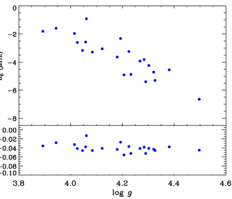
With this first application of the empirical surface correction to a large sample of solar-type stars, we can explore the behavior of the derived surface correction amplitude $a_{0}$ . We performed linear regressions to search for any correlation of $a_{0}$ with various combinations of $\log T_{\rm eff}$ , $\log g$ , and [Fe/H]. We identified a strong correlation with the asteroseismic $\log g$ (see upper panel of Figure 5), and statistically insignificant correlations with $T_{\rm eff}$ and metallicity. There may still be a correlation with $T_{\rm eff}$ , but the small 0.07 dex-range of $T_{\rm eff}$ in this sample (compared to the 0.6 dex-range in $\log g$ and 1.6 dex-range in [Fe/H]) makes it undetectable. In the lower panel of Figure 5 we show $a_{0}/\langle\Delta\nu\rangle$ versus $\log g$ , revealing that the distribution is relatively flat. This finding, that $a_{0}$ is roughly a fixed fraction of $\langle\Delta\nu\rangle$ for most stars, is entirely consistent with the conclusion by White et al. (2011b) that $\epsilon$ [the phase shift in the asymptotic relation, see their Eq. (1)] differs from theoretical models by a roughly constant offset. Whether these results will provide some insight into the deficiencies of stellar models relative to 3D convection simulations (Trampedach & Stein, 2011) remains to be seen.

5. CONCLUSIONS

We have completed the first uniform asteroseismic analysis of a large sample of 22 solar-type stars with the highest signal-to-noise ratio, observed for 1 month each during the first year of the Kepler mission. By fitting the individual frequencies instead of the global oscillation properties, we have improved the internal statistical precision on the derived values of the stellar radius, mass, and age. This result has implications for the study of exoplanet host stars, where these quantities can improve the characterization of the transiting planetary system. Although the absolute accuracy is more difficult to assess, the excellent agreement between the empirical scaling relations and several different fitting methods suggests that the systematic uncertainty is comparable to the statistical precision.

Adopting the results from the Asteroseismic Modeling Portal (AMP) as the reference for our comparisons, we quantified the precision and accuracy relative to AMP of asteroseismic determinations of radius, mass, and age that are possible using various methods. Empirical scaling relations based on the global oscillation properties ( $\langle\Delta\nu\rangle$ , $\nu_{\rm max}$ ) and $T_{\rm eff}$ can provide estimates of the stellar radius to a precision of 3% and the stellar mass to a precision of 9%. There is a tendency for scaling relations to slightly overestimate both the radius ( $+\,0.3\,\sigma$ ) and the mass ( $+\,0.4\,\sigma$ ) relative to AMP results (where $\sigma$ is the quadratic sum of the uncertainties from the two methods being compared). Model-grid-based methods can use additional observational constraints ( $\log g$ , [Fe/H], $L$ ) to achieve a radius precision as good as 1.4%, a mass precision of 4–6% and an age precision of 15–21%. These methods tend to slightly underestimate the radius (up to $-1.4\,\sigma$ ) and the mass (up to $-\,1.5\,\sigma$ ), while slightly overestimating the age (up to $+\,1.5\,\sigma$ ) compared to AMP results. AMP incorporates an empirical correction for surface effects (Kjeldsen et al., 2008) to provide a fit to the individual frequencies instead of the global oscillation properties by computing $\sim\,10^{5}$ models for each star, yielding a radius precision of 0.8%, a mass precision of 1.2% and an age precision of 2.5%. These results demonstrate that the precision gradually improves as more information is used in the fitting. An attempt to quantify the possible systematic errors associated with our treatment of surface effects resulted in mean offsets for the values of the adjustable model parameters for stars with clean mode ridges, ( $\Delta M\,=\,+0.01\,\ M_{\odot}$ , $\Delta t\,=\,-\,0.25$ Gyr, $\Delta Z\,=\,+\,0.0005$ , $\Delta Y_{\rm i}\,=\,+\,0.008$ , and $\Delta\alpha\,=\,-\,0.06$ ) that are comparable to the statistical uncertainties. By using the additional information contained in the individual frequencies, AMP also yields the stellar composition and mixing-length. Further improvements of the physics of the models such as including rotation and non-adiabatic effects may eliminate the necessity of using an empirical surface correction. The AMP website⁴⁴4The AMP website is at http://amp.ucar.edu/ contains an archive with complete details for the 22 models we present in this paper, including profiles of the interior structure and a full list of low-degree oscillation frequencies. The source code is also available⁵⁵5The AMP source code is at https://proxy.subversion.ucar.edu/AMP/, but as a service to the community it can be run directly on TeraGrid supercomputers from the website.

The largest outliers from our uniform model-fitting approach with AMP (see Tables 2.1 and 2) appear to arise from complications in the data analysis. Even with a careful procedure for validating the frequencies and the identification of modes extracted from the oscillation power spectrum, there remain some difficulties at the highest and lowest frequencies where the signal-to-noise ratio becomes marginal. One or two misidentified or spurious frequencies can boost the value of $\chi^{2}_{\rm seis}$ and bias the resulting model-fit. The longer data sets on these targets that will be obtained by Kepler in the future promise to improve the signal-to-noise ratio and resolve these few ambiguities. The typical values of the normalized $\chi^{2}_{\rm seis}$ are still larger than 1, which may be due to the physics used in the models but also to the influence of stellar magnetic cycles or underestimated uncertainties on the frequencies. Stellar activity is known to induce systematic shifts in the p-mode frequencies (García et al., 2010; Salabert et al., 2011) with a magnitude comparable to the typical statistical uncertainties for our sample. Stars observed near the the maximum of their magnetic cycles may show elevated values of the normalized $\chi^{2}_{\rm seis}$ and slight biases in their derived properties. The stars in our sample with the lowest metallicities ([Fe/H] $\,<\,-\,0.3$ ) presented the greatest challenge for AMP to reconcile the asteroseismic and spectroscopic constraints. This may be due to complications in the spectroscopic analysis for metal-poor stars, deficiencies in our stellar models at low metallicity, or both. Additional spectroscopic data and independent modeling efforts will ultimately address the source of these issues with low metallicity stars. The feedback loop between new asteroseismic observations and model development will gradually improve our understanding of stellar evolution.

After completing an asteroseismic survey of nearly 2000 solar-type stars during the first year of its mission, Kepler began collecting longer data sets for several hundred of the best targets. A preview of what is possible with extended observations can be found in Mathur et al. (2011), Campante et al. (2011), Creevey et al. (2012), Brandão et al. (in preparation) and Doğan et al. (in preparation), who performed analysis and modeling of several stars that were observed for 8 months during the survey phase of the mission. These targets are relatively faint compared to the brightest stars that are being observed during the specific target phase of the mission, so we can expect many new surprises as Kepler continues its census of the galactic neighborhood.

Funding for this Discovery mission is provided by NASA’s Science Mission Directorate. This work was supported in part by NASA grant NNX09AE59G and by White Dwarf Research Corporation through the Pale Blue Dot project. The authors wish to thank the entire Kepler team, without whom these results would not be possible. We also thank all funding councils and agencies that have supported the activities of KASC Working Group 1, and the International Space Science Institute (ISSI). The research leading to these results has received funding from the European Community’s Seventh Framework Programme (FP7/2007-2013) under grant agreement no. 269194 (IRSES/ASK). Computational time on Kraken at the National Institute of Computational Sciences was provided through NSF TeraGrid allocation TG-AST090107. Funding to integrate AMP with TeraGrid resources was provided by the TeraGrid Science Gateways program. Computational time at NCAR was provided by NSF MRI Grants CNS-0421498, CNS-0420873, and CNS-0420985, NSF sponsorship of the National Center for Atmospheric Research, the University of Colorado, and a grant from the IBM Shared University Research program.

References

Aerts et al. (2010) Aerts, C., Christensen-Dalsgaard, J., & Kurtz, D. W. 2010, Asteroseismology, ed. Aerts, C., Christensen-Dalsgaard, J., & Kurtz, D. W.
Alexander & Ferguson (1994) Alexander, D. R., & Ferguson, J. W. 1994, ApJ, 437, 879
Ammons et al. (2006) Ammons, S. M., Robinson, S. E., Strader, J., Laughlin, G., Fischer, D., & Wolf, A. 2006, ApJ, 638, 1004
Anderson et al. (1990) Anderson, E. R., Duvall, Jr., T. L., & Jefferies, S. M. 1990, ApJ, 364, 699
Ballot et al. (2011a) Ballot, J., Barban, C., & van’t Veer-Menneret, C. 2011a, A&A, 531, A124
Ballot et al. (2011b) Ballot, J., et al. 2011b, A&A, 530, A97
Basu et al. (2010) Basu, S., Chaplin, W. J., & Elsworth, Y. 2010, ApJ, 710, 1596
Basu et al. (2011) Basu, S., et al. 2011, ApJ, 729, L10
Bedding et al. (2011) Bedding, T. R., et al. 2011, Nature, 471, 608
Belkacem et al. (2011) Belkacem, K., Goupil, M. J., Dupret, M. A., Samadi, R., Baudin, F., Noels, A., & Mosser, B. 2011, A&A, 530, A142
Böhm-Vitense (1958) Böhm-Vitense, E. 1958, ZAp, 46, 108
Borucki et al. (2010) Borucki, W. J., et al. 2010, Science, 327, 977
Broomhall et al. (2010) Broomhall, A.-M., Chaplin, W. J., Elsworth, Y., Appourchaux, T., & New, R. 2010, MNRAS, 406, 767
Brown & Gilliland (1994) Brown, T. M., & Gilliland, R. L. 1994, ARA&A, 32, 37
Brown et al. (1991) Brown, T. M., Gilliland, R. L., Noyes, R. W., & Ramsey, L. W. 1991, ApJ, 368, 599
Brown et al. (2011) Brown, T. M., Latham, D. W., Everett, M. E., & Esquerdo, G. A. 2011, AJ, 142, 112
Broyden (1970) Broyden, C. 1970, Journal Inst. Math. Applic., 6, 76
Bruntt et al. (2010a) Bruntt, H., et al. 2010a, MNRAS, 405, 1907
Bruntt et al. (2010b) —. 2010b, A&A, 519, A51
Bruntt et al. (2011) —. 2011, MNRAS, submitted
Campante et al. (2011) Campante, T. L., et al. 2011, A&A, 534, A6
Casagrande et al. (2007) Casagrande, L., Flynn, C., Portinari, L., Girardi, L., & Jimenez, R. 2007, MNRAS, 382, 1516
Casagrande et al. (2010) Casagrande, L., Ramírez, I., Meléndez, J., Bessell, M., & Asplund, M. 2010, A&A, 512, A54
Chaplin et al. (2011) Chaplin, W. J., et al. 2011, Science, 332, 213
Christensen-Dalsgaard (2008a) Christensen-Dalsgaard, J. 2008a, Ap&SS, 316, 13
Christensen-Dalsgaard (2008b) —. 2008b, Ap&SS, 316, 113
Christensen-Dalsgaard et al. (2007) Christensen-Dalsgaard, J., Arentoft, T., Brown, T. M., Gilliland, R. L., Kjeldsen, H., Borucki, W. J., & Koch, D. 2007, Communications in Asteroseismology, 150, 350
Christensen-Dalsgaard & Thompson (1997) Christensen-Dalsgaard, J., & Thompson, M. J. 1997, MNRAS, 284, 527
Christensen-Dalsgaard et al. (2010) Christensen-Dalsgaard, J., et al. 2010, ApJ, 713, L164
Cox (2000) Cox, A. N. 2000, Allen’s astrophysical quantities (New York: AIP Press; Springer, 2000)
Creevey et al. (2012) Creevey, O. L., et al. 2012, A&A, 537, A111
Deheuvels et al. (2010) Deheuvels, S., et al. 2010, A&A, 515, A87
Demarque et al. (2008) Demarque, P., Guenther, D. B., Li, L. H., Mazumdar, A., & Straka, C. W. 2008, Ap&SS, 316, 31
Demarque et al. (2004) Demarque, P., Woo, J.-H., Kim, Y.-C., & Yi, S. K. 2004, ApJS, 155, 667
Dotter et al. (2008) Dotter, A., Chaboyer, B., Jevremović, D., Kostov, V., Baron, E., & Ferguson, J. W. 2008, ApJS, 178, 89
Eggleton et al. (1973) Eggleton, P. P., Faulkner, J., & Flannery, B. P. 1973, A&A, 23, 325
Fletcher (1970) Fletcher, R. 1970, Computer Journal, 13, 317
Flower (1996) Flower, P. J. 1996, ApJ, 469, 355
Gai et al. (2011) Gai, N., Basu, S., Chaplin, W. J., & Elsworth, Y. 2011, ApJ, 730, 63
García et al. (2010) García, R. A., Mathur, S., Salabert, D., Ballot, J., Régulo, C., Metcalfe, T. S., & Baglin, A. 2010, Science, 329, 1032
García et al. (2011) García, R. A., et al. 2011, MNRAS, 414, L6
Gaulme et al. (2010) Gaulme, P., et al. 2010, A&A, 524, A47
Gilliland et al. (2010) Gilliland, R. L., et al. 2010, ApJ, 713, L160
Goldfarb (1970) Goldfarb, D. 1970, Mathematics of Computing, 24, 23
Grevesse & Noels (1993) Grevesse, N., & Noels, A. 1993, in Origin and evolution of the elements: proceedings of a symposium in honour of H. Reeves, held in Paris, June 22-25, 1992. Edited by N. Prantzos, E. Vangioni-Flam and M. Casse. Published by Cambridge University Press, Cambridge, England, 1993, p.14, ed. N. Prantzos, E. Vangioni-Flam, & M. Casse, 14
Grevesse & Sauval (1998) Grevesse, N., & Sauval, A. J. 1998, Space Sci. Rev., 85, 161
Grigahcène et al. (2005) Grigahcène, A., Dupret, M.-A., Gabriel, M., Garrido, R., & Scuflaire, R. 2005, A&A, 434, 1055
Guenther & Brown (2004) Guenther, D. B., & Brown, K. I. T. 2004, ApJ, 600, 419
Handberg & Campante (2011) Handberg, R., & Campante, T. L. 2011, A&A, 527, A56
Harvey (1985) Harvey, J. 1985, in ESA Special Publication, Vol. 235, Future Missions in Solar, Heliospheric & Space Plasma Physics, ed. E. Rolfe & B. Battrick, 199
Hazlewood & Woitaszek (2011) Hazlewood, V., & Woitaszek, M. 2011, in TeraGrid 2011, Salt Lake City, Utah, USA
Huber et al. (2010) Huber, D., et al. 2010, ApJ, 723, 1607
Iglesias & Rogers (1996) Iglesias, C. A., & Rogers, F. J. 1996, ApJ, 464, 943
Jenkins et al. (2010) Jenkins, J. M., et al. 2010, ApJ, 713, L87
Kjeldsen & Bedding (1995) Kjeldsen, H., & Bedding, T. R. 1995, A&A, 293, 87
Kjeldsen et al. (2008) Kjeldsen, H., Bedding, T. R., & Christensen-Dalsgaard, J. 2008, ApJ, 683, L175
Kurucz (1991) Kurucz, R. L. 1991, in NATO ASIC Proc. 341: Stellar Atmospheres - Beyond Classical Models, ed. L. Crivellari, I. Hubeny, & D. G. Hummer, 441
Marigo et al. (2008) Marigo, P., Girardi, L., Bressan, A., Groenewegen, M. A. T., Silva, L., & Granato, G. L. 2008, A&A, 482, 883
Mathur et al. (2011) Mathur, S., et al. 2011, ApJ, 733, 95
Metcalfe & Charbonneau (2003) Metcalfe, T. S., & Charbonneau, P. 2003, Journal of Computational Physics, 185, 176
Metcalfe et al. (2009) Metcalfe, T. S., Creevey, O. L., & Christensen-Dalsgaard, J. 2009, ApJ, 699, 373
Metcalfe et al. (2010) Metcalfe, T. S., et al. 2010, ApJ, 723, 1583
Michaud & Proffitt (1993) Michaud, G., & Proffitt, C. R. 1993, in Astronomical Society of the Pacific Conference Series, Vol. 40, IAU Colloq. 137: Inside the Stars, ed. W. W. Weiss & A. Baglin, 246–259
Moya et al. (2010) Moya, A., Amado, P. J., Barrado, D., García Hernández, A., Aberasturi, M., Montesinos, B., & Aceituno, F. 2010, MNRAS, 405, L81
Peirce (1852) Peirce, B. 1852, AJ, 2, 161
Pinsonneault et al. (2011) Pinsonneault, M., An, D., Molenda-Żakowicz, J., Chaplin, W. J., Metcalfe, T. S., & Bruntt, H. 2011, ApJ, submitted
Quirion et al. (2010) Quirion, P.-O., Christensen-Dalsgaard, J., & Arentoft, T. 2010, ApJ, 725, 2176
Rogers & Iglesias (1995) Rogers, F. J., & Iglesias, C. A. 1995, in Astronomical Society of the Pacific Conference Series, Vol. 78, Astrophysical Applications of Powerful New Databases, ed. S. J. Adelman & W. L. Wiese, 31
Rogers & Nayfonov (2002) Rogers, F. J., & Nayfonov, A. 2002, ApJ, 576, 1064
Salabert et al. (2011) Salabert, D., Régulo, C., Ballot, J., García, R. A., & Mathur, S. 2011, A&A, 530, A127
Shanno (1970) Shanno, D. 1970, Mathematics of Computing, 24, 647
Soderblom (2010) Soderblom, D. R. 2010, ARA&A, 48, 581
Spergel et al. (2007) Spergel, D. N., et al. 2007, ApJS, 170, 377
Stello et al. (2009a) Stello, D., Chaplin, W. J., Basu, S., Elsworth, Y., & Bedding, T. R. 2009a, MNRAS, 400, L80
Stello et al. (2009b) Stello, D., et al. 2009b, ApJ, 700, 1589
Stello et al. (2010) —. 2010, ApJ, 713, L182
Suárez et al. (2010) Suárez, J. C., Goupil, M. J., Reese, D. R., Samadi, R., Lignières, F., Rieutord, M., & Lochard, J. 2010, ApJ, 721, 537
Torres (2010) Torres, G. 2010, AJ, 140, 1158
Toutain & Appourchaux (1994) Toutain, T., & Appourchaux, T. 1994, A&A, 289, 649
Trampedach & Stein (2011) Trampedach, R., & Stein, R. F. 2011, ApJ, 731, 78
Troisi et al. (2011) Troisi, F., et al. 2011, PASP, 123, 879
van Leeuwen (2007a) van Leeuwen, F. 2007a, Astrophysics and Space Science Library, Vol. 350, Hipparcos, the New Reduction of the Raw Data, ed. F. van Leeuwen
van Leeuwen (2007b) —. 2007b, A&A, 474, 653
Verner et al. (2011) Verner, G. A., et al. 2011, MNRAS, 892
White et al. (2011a) White, T. R., Bedding, T. R., Stello, D., Christensen-Dalsgaard, J., Huber, D., & Kjeldsen, H. 2011a, ApJ, 743, 161
White et al. (2011b) White, T. R., et al. 2011b, ApJ, 742, L3
Woitaszek et al. (2009) Woitaszek, M., Metcalfe, T., & Shorrock, I. 2009, in GCE ’09: Proceedings of the 5th Grid Computing Environments Workshop, Portland, Oregon, USA, 1–7

Appendix A A. FREQUENCY TABLES

Observed and model frequencies for KIC 3632418⁺⁺ $\nu_{\rm obs}$ is the observed frequency, $\nu_{\rm corr}$ is the model frequency from AMP after applying the surface corrections, and $a_{\nu}$ is the size of the surface correction. Same note apply to Tables A to A.

$\ell$	$n\tablenotemark{*}$	$\nu_{\rm obs}$ ( $\mu$ Hz)	$\nu_{\rm corr}$ ( $\mu$ Hz)	$a_{\nu}$ ( $\mu$ Hz)
0	10	$\cdots$	679.65	$-$ 0.24
0	11	$\cdots$	737.76	$-$ 0.34
0	12	$\cdots$	796.24	$-$ 0.48
0	13	$856.50\pm 0.61$	856.79	$-$ 0.65
0	14	$918.59\pm 0.42$	917.42	$-$ 0.88
0	15	$979.48\pm 0.38$	978.29	$-$ 1.15
0	16	$1039.31\pm 0.35$	1038.03	$-$ 1.49
0	17	$1098.75\pm 0.42$	1098.89	$-$ 1.90
0	18	$1158.95\pm 0.34$	1159.75	$-$ 2.40
0	19	$1221.73\pm 0.36$	1221.67	$-$ 3.01
0	20	$1282.72\pm 0.32$	1282.92	$-$ 3.71
0	21	$1340.86\pm 0.39$	1344.34	$-$ 4.55
0	22	$1404.69\pm 0.53$	1405.35	$-$ 5.51
0	23	$1467.09\pm 0.46$	1466.45	$-$ 6.63
0	24	$\cdots$	1527.60	$-$ 7.92
0	25	$\cdots$	1588.33	$-$ 9.39
1	10	$\cdots$	705.74	$-$ 0.28
1	11	$\cdots$	763.37	$-$ 0.40
1	12	$\cdots$	823.02	$-$ 0.55
1	13	$884.65\pm 0.60$	883.45	$-$ 0.74
1	14	$947.70\pm 0.92$	944.35	$-$ 0.99
1	15	$1005.31\pm 0.37$	1004.47	$-$ 1.29
1	16	$1064.46\pm 0.39$	1064.57	$-$ 1.66
1	17	$1125.57\pm 0.36$	1125.44	$-$ 2.11
1	18	$1187.57\pm 0.39$	1186.66	$-$ 2.65
1	19	$1248.38\pm 0.45$	1248.50	$-$ 3.30
1	20	$1308.33\pm 0.35$	1309.58	$-$ 4.06
1	21	$1371.44\pm 0.37$	1371.09	$-$ 4.95
1	22	$1431.96\pm 0.50$	1431.88	$-$ 5.98
1	23	$\cdots$	1493.34	$-$ 7.18
1	24	$\cdots$	1554.14	$-$ 8.54
1	25	$\cdots$	1615.22	$-$ 10.10
2	10	$\cdots$	733.46	$-$ 0.34
2	11	$\cdots$	791.54	$-$ 0.46
2	12	$849.94\pm 0.79$	852.08	$-$ 0.64
2	13	$\cdots$	912.69	$-$ 0.86
2	14	$974.52\pm 0.45$	973.66	$-$ 1.13
2	15	$1033.86\pm 0.41$	1033.41	$-$ 1.46
2	16	$1095.32\pm 0.45$	1094.23	$-$ 1.87
2	17	$1154.85\pm 0.46$	1155.10	$-$ 2.36
2	18	$1215.82\pm 0.50$	1217.00	$-$ 2.96
2	19	$1277.83\pm 0.44$	1278.38	$-$ 3.66
2	20	$\cdots$	1339.81	$-$ 4.48
2	21	$1399.98\pm 0.76$	1400.99	$-$ 5.44
2	22	$1462.06\pm 0.48$	1462.11	$-$ 6.55
2	23	$\cdots$	1523.45	$-$ 7.83
2	24	$\cdots$	1584.27	$-$ 9.29
2	25	$\cdots$	1645.33	$-$ 10.96

Observed and model frequencies for KIC 3656476

$\ell$	$n$	$\nu_{\rm obs}$ ( $\mu$ Hz)	$\nu_{\rm corr}$ ( $\mu$ Hz)	$a_{\nu}$ ( $\mu$ Hz)
0	14	$\cdots$	1442.87	$-$ 1.39
0	15	$\cdots$	1535.03	$-$ 1.81
0	16	$\cdots$	1626.69	$-$ 2.32
0	17	1719.75 $\pm$ 0.23	1719.21	$-$ 2.95
0	18	1812.50 $\pm$ 0.14	1812.61	$-$ 3.70
0	19	1905.16 $\pm$ 0.30	1905.82	$-$ 4.59
0	20	1998.70 $\pm$ 0.13	1998.96	$-$ 5.65
0	21	2092.69 $\pm$ 0.26	2092.17	$-$ 6.88
0	22	$\cdots$	2185.27	$-$ 8.30
0	23	$\cdots$	2278.73	$-$ 9.96
1	14	$\cdots$	1483.50	$-$ 1.56
1	15	$\cdots$	1575.36	$-$ 2.02
1	16	1668.63 $\pm$ 0.20	1667.71	$-$ 2.58
1	17	1761.00 $\pm$ 0.20	1760.72	$-$ 3.26
1	18	1854.17 $\pm$ 0.08	1854.30	$-$ 4.08
1	19	1947.69 $\pm$ 0.24	1947.88	$-$ 5.05
1	20	2040.96 $\pm$ 0.15	2041.06	$-$ 6.18
1	21	2134.21 $\pm$ 0.22	2134.50	$-$ 7.50
1	22	$\cdots$	2228.16	$-$ 9.03
1	23	$\cdots$	2321.71	$-$ 10.80
2	14	$\cdots$	1529.09	$-$ 1.78
2	15	$\cdots$	1620.93	$-$ 2.29
2	16	$\cdots$	1713.70	$-$ 2.91
2	17	1807.82 $\pm$ 0.14	1807.36	$-$ 3.65
2	18	1901.10 $\pm$ 0.23	1900.86	$-$ 4.54
2	19	1994.28 $\pm$ 0.16	1994.36	$-$ 5.59
2	20	2088.39 $\pm$ 0.29	2087.88	$-$ 6.81
2	21	$\cdots$	2181.32	$-$ 8.24
2	22	$\cdots$	2275.15	$-$ 9.89
2	23	$\cdots$	2368.99	$-$ 11.79

Observed and model frequencies for KIC 4914923

$\ell$	$n$	$\nu_{\rm obs}$ ( $\mu$ Hz)	$\nu_{\rm corr}$ ( $\mu$ Hz)	$a_{\nu}$ ( $\mu$ Hz)
0	13	$\cdots$	1276.12	$-$ 1.04
0	14	$\cdots$	1364.28	$-$ 1.39
0	15	$\cdots$	1451.43	$-$ 1.81
0	16	$\cdots$	1538.78	$-$ 2.32
0	17	1626.83 $\pm$ 0.77	1626.76	$-$ 2.95
0	18	1715.26 $\pm$ 0.24	1715.67	$-$ 3.72
0	19	1804.44 $\pm$ 0.30	1804.51	$-$ 4.62
0	20	1893.09 $\pm$ 0.33	1893.02	$-$ 5.68
0	21	1981.63 $\pm$ 0.33	1981.73	$-$ 6.93
0	22	2070.74 $\pm$ 0.30	2070.32	$-$ 8.38
0	23	$\cdots$	2159.22	$-$ 10.05
0	24	$\cdots$	2248.07	$-$ 11.98
1	13	$\cdots$	1314.87	$-$ 1.18
1	14	$\cdots$	1402.85	$-$ 1.56
1	15	1491.40 $\pm$ 0.24	1489.86	$-$ 2.02
1	16	1577.98 $\pm$ 0.12	1577.59	$-$ 2.59
1	17	1666.62 $\pm$ 0.49	1666.31	$-$ 3.28
1	18	1755.24 $\pm$ 0.28	1755.23	$-$ 4.10
1	19	1844.23 $\pm$ 0.32	1844.26	$-$ 5.08
1	20	1932.32 $\pm$ 0.30	1932.91	$-$ 6.22
1	21	2021.42 $\pm$ 0.30	2021.73	$-$ 7.55
1	22	$\cdots$	2110.80	$-$ 9.11
1	23	$\cdots$	2199.71	$-$ 10.90
1	24	$\cdots$	2288.79	$-$ 12.96
2	13	$\cdots$	1357.97	$-$ 1.36
2	14	$\cdots$	1445.35	$-$ 1.78
2	15	$\cdots$	1532.79	$-$ 2.29
2	16	1619.51 $\pm$ 0.90	1620.88	$-$ 2.91
2	17	1709.17 $\pm$ 0.33	1710.00	$-$ 3.66
2	18	1799.55 $\pm$ 0.17	1799.04	$-$ 4.56
2	19	1886.13 $\pm$ 0.22	1887.82	$-$ 5.62
2	20	1976.24 $\pm$ 0.23	1976.78	$-$ 6.85
2	21	$\cdots$	2065.62	$-$ 8.29
2	22	$\cdots$	2154.82	$-$ 9.96
2	23	$\cdots$	2243.94	$-$ 11.89
2	24	$\cdots$	2332.79	$-$ 14.08

Observed and model frequencies for KIC 5184732

$\ell$	$n$	$\nu_{\rm obs}$ ( $\mu$ Hz)	$\nu_{\rm corr}$ ( $\mu$ Hz)	$a_{\nu}$ ( $\mu$ Hz)
0	13	$\cdots$	1376.70	$-$ 0.69
0	14	$\cdots$	1472.42	$-$ 0.92
0	15	$\cdots$	1568.22	$-$ 1.21
0	16	1661.99 $\pm$ 0.26	1662.74	$-$ 1.56
0	17	1757.40 $\pm$ 0.22	1756.60	$-$ 1.97
0	18	1851.65 $\pm$ 0.32	1851.20	$-$ 2.47
0	19	1946.49 $\pm$ 0.30	1946.45	$-$ 3.06
0	20	2042.89 $\pm$ 0.23	2042.45	$-$ 3.77
0	21	2138.02 $\pm$ 0.26	2138.20	$-$ 4.59
0	22	2234.82 $\pm$ 0.28	2233.65	$-$ 5.55
0	23	2329.25 $\pm$ 0.21	2329.26	$-$ 6.65
0	24	2424.02 $\pm$ 0.22	2424.69	$-$ 7.91
0	25	2518.26 $\pm$ 0.41	2520.59	$-$ 9.36
0	26	$\cdots$	2616.39	$-$ 11.00
0	27	$\cdots$	2712.03	$-$ 12.86
1	13	$\cdots$	1420.43	$-$ 0.79
1	14	$\cdots$	1516.55	$-$ 1.05
1	15	1612.73 $\pm$ 0.14	1611.79	$-$ 1.36
1	16	1705.47 $\pm$ 0.29	1706.26	$-$ 1.74
1	17	1801.06 $\pm$ 0.27	1800.39	$-$ 2.19
1	18	1895.75 $\pm$ 0.26	1895.61	$-$ 2.73
1	19	1991.29 $\pm$ 0.26	1991.66	$-$ 3.38
1	20	2087.57 $\pm$ 0.18	2087.69	$-$ 4.14
1	21	2182.61 $\pm$ 0.33	2183.82	$-$ 5.03
1	22	2278.57 $\pm$ 0.26	2279.48	$-$ 6.05
1	23	2374.59 $\pm$ 0.16	2375.35	$-$ 7.24
1	24	2471.22 $\pm$ 0.25	2471.47	$-$ 8.59
1	25	2570.78 $\pm$ 0.74	2567.48	$-$ 10.13
1	26	$\cdots$	2663.79	$-$ 11.89
1	27	$\cdots$	2759.62	$-$ 13.87
2	13	$\cdots$	1465.02	$-$ 0.90
2	14	$\cdots$	1561.02	$-$ 1.19
2	15	1655.03 $\pm$ 0.39	1655.73	$-$ 1.53
2	16	1749.44 $\pm$ 0.32	1749.83	$-$ 1.94
2	17	1844.33 $\pm$ 0.22	1844.55	$-$ 2.43
2	18	1940.21 $\pm$ 0.35	1939.99	$-$ 3.02
2	19	2036.42 $\pm$ 0.30	2036.28	$-$ 3.72
2	20	2133.04 $\pm$ 0.45	2132.29	$-$ 4.54
2	21	2229.00 $\pm$ 0.34	2228.10	$-$ 5.49
2	22	2326.08 $\pm$ 0.40	2324.00	$-$ 6.58
2	23	2419.70 $\pm$ 0.86	2419.73	$-$ 7.84
2	24	$\cdots$	2515.98	$-$ 9.28
2	25	$\cdots$	2612.08	$-$ 10.92
2	26	$\cdots$	2708.08	$-$ 12.78
2	27	$\cdots$	2804.07	$-$ 14.87

Observed and model frequencies for KIC 5512589

$\ell$	$n$	$\nu_{\rm obs}$ ( $\mu$ Hz)	$\nu_{\rm corr}$ ( $\mu$ Hz)	$a_{\nu}$ ( $\mu$ Hz)
0	11	$\cdots$	846.20	$-$ 0.50
0	12	$\cdots$	914.19	$-$ 0.70
0	13	$\cdots$	981.66	$-$ 0.95
0	14	$\cdots$	1048.46	$-$ 1.26
0	15	$\cdots$	1115.80	$-$ 1.64
0	16	1184.09 $\pm$ 0.33	1183.92	$-$ 2.12
0	17	1252.54 $\pm$ 0.37	1252.37	$-$ 2.71
0	18	1321.08 $\pm$ 0.20	1320.77	$-$ 3.40
0	19	$\cdots$	1389.05	$-$ 4.23
0	20	1456.89 $\pm$ 0.20	1457.55	$-$ 5.21
0	21	$\cdots$	1526.25	$-$ 6.37
0	22	$\cdots$	1594.88	$-$ 7.71
1	11	$\cdots$	877.12	$-$ 0.58
1	12	$\cdots$	944.19	$-$ 0.80
1	13	1010.26 $\pm$ 0.24	1010.94	$-$ 1.08
1	14	1077.93 $\pm$ 0.23	1077.50	$-$ 1.42
1	15	1145.16 $\pm$ 0.29	1144.93	$-$ 1.84
1	16	1212.63 $\pm$ 0.27	1213.18	$-$ 2.36
1	17	1281.51 $\pm$ 0.40	1281.43	$-$ 2.99
1	18	1349.42 $\pm$ 0.35	1349.64	$-$ 3.74
1	19	1418.84 $\pm$ 0.27	1417.98	$-$ 4.63
1	20	1486.16 $\pm$ 0.24	1486.45	$-$ 5.68
1	21	$\cdots$	1555.14	$-$ 6.91
1	22	$\cdots$	1623.78	$-$ 8.33
2	11	$\cdots$	976.18	$-$ 0.93
2	12	$\cdots$	1043.09	$-$ 1.23
2	13	$\cdots$	1110.42	$-$ 1.61
2	14	1178.50 $\pm$ 0.31	1178.48	$-$ 2.08
2	15	1246.45 $\pm$ 0.28	1246.49	$-$ 2.65
2	16	$\cdots$	1275.37	$-$ 2.93
2	17	1315.78 $\pm$ 0.21	1316.39	$-$ 3.35
2	18	1384.28 $\pm$ 0.37	1384.42	$-$ 4.17
2	19	1451.69 $\pm$ 0.25	1452.98	$-$ 5.14
2	20	$\cdots$	1521.76	$-$ 6.28
2	21	$\cdots$	1590.52	$-$ 7.62
2	22	$\cdots$	1659.28	$-$ 9.16

Observed and model frequencies for KIC 6106415

$\ell$	$n$	$\nu_{\rm obs}$ ( $\mu$ Hz)	$\nu_{\rm corr}$ ( $\mu$ Hz)	$a_{\nu}$ ( $\mu$ Hz)
0	13	$\cdots$	1497.25	$-$ 0.70
0	14	$\cdots$	1601.16	$-$ 0.93
0	15	$\cdots$	1704.69	$-$ 1.21
0	16	1807.96 $\pm$ 0.39	1807.03	$-$ 1.56
0	17	1910.30 $\pm$ 0.26	1909.72	$-$ 1.98
0	18	2012.90 $\pm$ 0.26	2013.26	$-$ 2.48
0	19	2118.00 $\pm$ 0.30	2117.43	$-$ 3.08
0	20	2221.41 $\pm$ 0.18	2221.81	$-$ 3.79
0	21	2325.32 $\pm$ 0.32	2325.86	$-$ 4.62
0	22	2429.08 $\pm$ 0.31	2430.12	$-$ 5.58
0	23	2534.38 $\pm$ 0.73	2534.44	$-$ 6.69
0	24	2638.90 $\pm$ 0.26	2639.04	$-$ 7.97
0	25	2743.07 $\pm$ 0.20	2743.73	$-$ 9.44
0	26	$\cdots$	2848.29	$-$ 11.10
0	27	$\cdots$	2952.85	$-$ 12.98
1	13	$\cdots$	1544.71	$-$ 0.80
1	14	$\cdots$	1648.65	$-$ 1.05
1	15	1752.63 $\pm$ 0.43	1751.72	$-$ 1.37
1	16	1855.04 $\pm$ 0.50	1854.36	$-$ 1.74
1	17	1957.84 $\pm$ 0.30	1957.46	$-$ 2.20
1	18	2060.89 $\pm$ 0.20	2061.73	$-$ 2.75
1	19	2166.23 $\pm$ 0.22	2166.16	$-$ 3.40
1	20	2270.09 $\pm$ 0.27	2270.64	$-$ 4.17
1	21	2374.17 $\pm$ 0.32	2374.97	$-$ 5.06
1	22	2478.74 $\pm$ 0.22	2479.36	$-$ 6.09
1	23	2582.75 $\pm$ 0.20	2584.11	$-$ 7.28
1	24	2688.70 $\pm$ 0.20	2688.84	$-$ 8.64
1	25	$\cdots$	2793.73	$-$ 10.20
1	26	$\cdots$	2898.39	$-$ 11.97
1	27	$\cdots$	3002.96	$-$ 13.96
2	13	$\cdots$	1593.10	$-$ 0.91
2	14	$\cdots$	1696.85	$-$ 1.19
2	15	$\cdots$	1799.39	$-$ 1.53
2	16	1902.18 $\pm$ 0.30	1902.25	$-$ 1.95
2	17	2006.72 $\pm$ 0.33	2005.92	$-$ 2.44
2	18	2111.65 $\pm$ 1.43	2110.34	$-$ 3.04
2	19	2213.81 $\pm$ 0.30	2214.97	$-$ 3.74
2	20	2319.41 $\pm$ 0.47	2319.30	$-$ 4.56
2	21	2423.39 $\pm$ 0.28	2423.82	$-$ 5.52
2	22	2527.51 $\pm$ 0.28	2528.38	$-$ 6.63
2	23	2632.08 $\pm$ 0.55	2633.27	$-$ 7.90
2	24	2738.48 $\pm$ 1.07	2738.21	$-$ 9.35
2	25	$\cdots$	2843.05	$-$ 11.01
2	26	$\cdots$	2947.86	$-$ 12.88
2	27	$\cdots$	3052.37	$-$ 14.99

Observed and model frequencies for KIC 6116048

$\ell$	$n$	$\nu_{\rm obs}$ ( $\mu$ Hz)	$\nu_{\rm corr}$ ( $\mu$ Hz)	$a_{\nu}$ ( $\mu$ Hz)
0	13	$\cdots$	1448.56	$-$ 0.75
0	14	$\cdots$	1549.10	$-$ 1.00
0	15	1650.26 $\pm$ 0.24	1648.95	$-$ 1.31
0	16	1747.66 $\pm$ 0.34	1748.03	$-$ 1.68
0	17	1847.35 $\pm$ 0.25	1847.82	$-$ 2.13
0	18	1948.04 $\pm$ 0.28	1948.25	$-$ 2.68
0	19	2048.94 $\pm$ 0.21	2049.32	$-$ 3.33
0	20	2150.34 $\pm$ 0.24	2150.21	$-$ 4.10
0	21	2249.91 $\pm$ 0.17	2251.07	$-$ 4.99
0	22	2351.45 $\pm$ 0.19	2352.11	$-$ 6.04
0	23	2452.29 $\pm$ 0.23	2453.26	$-$ 7.24
0	24	2556.29 $\pm$ 0.57	2554.67	$-$ 8.63
0	25	$\cdots$	2655.93	$-$ 10.21
0	26	$\cdots$	2757.23	$-$ 12.02
1	13	$\cdots$	1494.19	$-$ 0.86
1	14	$\cdots$	1594.46	$-$ 1.13
1	15	1692.68 $\pm$ 0.34	1694.19	$-$ 1.47
1	16	1793.30 $\pm$ 0.26	1793.61	$-$ 1.88
1	17	1892.81 $\pm$ 0.32	1893.92	$-$ 2.37
1	18	1994.81 $\pm$ 0.35	1995.02	$-$ 2.97
1	19	2096.10 $\pm$ 0.24	2096.16	$-$ 3.67
1	20	2196.79 $\pm$ 0.30	2197.36	$-$ 4.50
1	21	2297.39 $\pm$ 0.17	2298.39	$-$ 5.46
1	22	2399.20 $\pm$ 0.23	2399.78	$-$ 6.58
1	23	2501.36 $\pm$ 0.15	2501.21	$-$ 7.87
1	24	2602.15 $\pm$ 0.73	2602.76	$-$ 9.36
1	25	$\cdots$	2704.26	$-$ 11.04
1	26	$\cdots$	2805.56	$-$ 12.96
2	13	$\cdots$	1541.40	$-$ 0.98
2	14	$\cdots$	1641.42	$-$ 1.28
2	15	$\cdots$	1740.73	$-$ 1.65
2	16	1840.35 $\pm$ 0.27	1840.65	$-$ 2.10
2	17	1941.93 $\pm$ 0.22	1941.27	$-$ 2.64
2	18	2042.93 $\pm$ 0.28	2042.59	$-$ 3.29
2	19	$\cdots$	2143.74	$-$ 4.05
2	20	2242.98 $\pm$ 0.19	2244.90	$-$ 4.94
2	21	2345.13 $\pm$ 0.18	2346.19	$-$ 5.97
2	22	2446.48 $\pm$ 0.21	2447.62	$-$ 7.17
2	23	$\cdots$	2549.30	$-$ 8.55
2	24	$\cdots$	2650.84	$-$ 10.13
2	25	$\cdots$	2752.43	$-$ 11.92
2	26	$\cdots$	2853.75	$-$ 13.95

Observed and model frequencies for KIC 6603624

$\ell$	$n$	$\nu_{\rm obs}$ ( $\mu$ Hz)	$\nu_{\rm corr}$ ( $\mu$ Hz)	$a_{\nu}$ ( $\mu$ Hz)
0	16	$\cdots$	1927.24	$-$ 1.84
0	17	$\cdots$	2036.29	$-$ 2.33
0	18	2146.80 $\pm$ 0.24	2146.45	$-$ 2.92
0	19	2256.65 $\pm$ 0.19	2256.81	$-$ 3.62
0	20	2367.18 $\pm$ 0.16	2367.11	$-$ 4.45
0	21	2477.43 $\pm$ 0.26	2477.54	$-$ 5.42
0	22	2587.77 $\pm$ 0.30	2587.93	$-$ 6.54
0	23	$\cdots$	2698.61	$-$ 7.84
0	24	$\cdots$	2809.61	$-$ 9.33
0	25	$\cdots$	2920.45	$-$ 11.03
1	16	$\cdots$	1977.72	$-$ 2.05
1	17	$\cdots$	2087.55	$-$ 2.59
1	18	2198.45 $\pm$ 0.25	2198.06	$-$ 3.23
1	19	2308.94 $\pm$ 0.11	2308.91	$-$ 4.00
1	20	2419.42 $\pm$ 0.22	2419.43	$-$ 4.89
1	21	2530.33 $\pm$ 0.18	2530.01	$-$ 5.93
1	22	2640.34 $\pm$ 0.25	2640.94	$-$ 7.14
1	23	2751.55 $\pm$ 0.22	2751.91	$-$ 8.53
1	24	$\cdots$	2863.04	$-$ 10.12
1	25	$\cdots$	2974.22	$-$ 11.94
2	16	$\cdots$	2030.22	$-$ 2.30
2	17	$\cdots$	2140.71	$-$ 2.89
2	18	2252.16 $\pm$ 0.20	2251.40	$-$ 3.59
2	19	2362.09 $\pm$ 0.19	2362.10	$-$ 4.41
2	20	$\cdots$	2472.89	$-$ 5.37
2	21	2583.10 $\pm$ 0.24	2583.59	$-$ 6.49
2	22	$\cdots$	2694.64	$-$ 7.79
2	23	$\cdots$	2805.95	$-$ 9.28
2	24	$\cdots$	2917.10	$-$ 10.98
2	25	$\cdots$	3028.28	$-$ 12.91

Observed and model frequencies for KIC 6933899

$\ell$	$n$	$\nu_{\rm obs}$ ( $\mu$ Hz)	$\nu_{\rm corr}$ ( $\mu$ Hz)	$a_{\nu}$ ( $\mu$ Hz)
0	12	$\cdots$	964.47	$-$ 0.73
0	13	$\cdots$	1036.06	$-$ 0.99
0	14	1108.35 $\pm$ 0.23	1107.03	$-$ 1.32
0	15	$\cdots$	1177.69	$-$ 1.72
0	16	1248.76 $\pm$ 0.26	1249.27	$-$ 2.21
0	17	1321.90 $\pm$ 0.20	1321.86	$-$ 2.82
0	18	1393.80 $\pm$ 0.28	1394.23	$-$ 3.56
0	19	1466.05 $\pm$ 0.26	1466.45	$-$ 4.42
0	20	1538.53 $\pm$ 0.29	1538.74	$-$ 5.45
0	21	$\cdots$	1611.01	$-$ 6.65
0	22	$\cdots$	1683.57	$-$ 8.05
0	23	$\cdots$	1756.06	$-$ 9.67
1	12	$\cdots$	996.14	$-$ 0.84
1	13	$\cdots$	1067.13	$-$ 1.12
1	14	$\cdots$	1137.39	$-$ 1.48
1	15	1208.28 $\pm$ 0.24	1208.41	$-$ 1.92
1	16	1280.00 $\pm$ 0.21	1280.25	$-$ 2.46
1	17	1352.56 $\pm$ 0.29	1352.66	$-$ 3.12
1	18	1424.84 $\pm$ 0.30	1425.02	$-$ 3.91
1	19	1496.21 $\pm$ 0.28	1497.01	$-$ 4.84
1	20	1568.85 $\pm$ 0.20	1569.29	$-$ 5.93
1	21	1642.44 $\pm$ 0.48	1641.74	$-$ 7.22
1	22	$\cdots$	1714.18	$-$ 8.71
1	23	$\cdots$	1786.67	$-$ 10.43
2	12	$\cdots$	1101.35	$-$ 1.29
2	13	$\cdots$	1171.81	$-$ 1.68
2	14	$\cdots$	1226.40	$-$ 2.05
2	15	1245.11 $\pm$ 0.31	1244.98	$-$ 2.18
2	16	1317.14 $\pm$ 0.35	1316.70	$-$ 2.78
2	17	1388.62 $\pm$ 0.42	1389.06	$-$ 3.50
2	18	1461.93 $\pm$ 0.27	1461.40	$-$ 4.36
2	19	$\cdots$	1533.75	$-$ 5.37
2	20	$\cdots$	1606.13	$-$ 6.56
2	21	$\cdots$	1678.85	$-$ 7.95
2	22	$\cdots$	1751.47	$-$ 9.56
2	23	$\cdots$	1823.86	$-$ 11.41

Observed and model frequencies for KIC 7680114

$\ell$	$n$	$\nu_{\rm obs}$ ( $\mu$ Hz)	$\nu_{\rm corr}$ ( $\mu$ Hz)	$a_{\nu}$ ( $\mu$ Hz)
0	12	$\cdots$	1141.41	$-$ 0.47
0	13	$\cdots$	1226.52	$-$ 0.63
0	14	$\cdots$	1311.38	$-$ 0.84
0	15	1395.31 $\pm$ 0.34	1395.12	$-$ 1.10
0	16	$\cdots$	1479.03	$-$ 1.42
0	17	1563.84 $\pm$ 0.23	1563.69	$-$ 1.80
0	18	$\cdots$	1648.91	$-$ 2.26
0	19	1734.23 $\pm$ 0.20	1734.39	$-$ 2.81
0	20	$\cdots$	1819.51	$-$ 3.45
0	21	1904.40 $\pm$ 0.42	1904.78	$-$ 4.21
0	22	$\cdots$	1990.31	$-$ 5.09
0	23	$\cdots$	2075.82	$-$ 6.10
1	12	$\cdots$	1178.87	$-$ 0.53
1	13	$\cdots$	1263.91	$-$ 0.72
1	14	1348.35 $\pm$ 0.34	1348.40	$-$ 0.95
1	15	1431.62 $\pm$ 0.35	1432.23	$-$ 1.23
1	16	$\cdots$	1516.41	$-$ 1.58
1	17	1601.26 $\pm$ 0.20	1601.72	$-$ 1.99
1	18	1686.44 $\pm$ 0.22	1687.21	$-$ 2.49
1	19	1773.26 $\pm$ 0.16	1772.69	$-$ 3.09
1	20	1856.72 $\pm$ 0.21	1858.23	$-$ 3.78
1	21	1943.50 $\pm$ 0.43	1943.70	$-$ 4.59
1	22	$\cdots$	2029.62	$-$ 5.53
1	23	$\cdots$	2115.60	$-$ 6.62
2	12	$\cdots$	1220.39	$-$ 0.62
2	13	$\cdots$	1305.43	$-$ 0.83
2	14	$\cdots$	1389.39	$-$ 1.08
2	15	$\cdots$	1473.48	$-$ 1.39
2	16	1558.10 $\pm$ 0.30	1558.27	$-$ 1.77
2	17	$\cdots$	1643.74	$-$ 2.23
2	18	1729.78 $\pm$ 0.19	1729.50	$-$ 2.78
2	19	$\cdots$	1814.90	$-$ 3.42
2	20	1900.20 $\pm$ 0.26	1900.50	$-$ 4.17
2	21	$\cdots$	1986.34	$-$ 5.04
2	22	$\cdots$	2072.21	$-$ 6.05
2	23	$\cdots$	2158.38	$-$ 7.22

Observed and model frequencies for KIC 7976303

$\ell$	$n$	$\nu_{\rm obs}$ ( $\mu$ Hz)	$\nu_{\rm corr}$ ( $\mu$ Hz)	$a_{\nu}$ ( $\mu$ Hz)
0	7	$\cdots$	428.79	$-$ 0.07
0	8	$\cdots$	479.66	$-$ 0.12
0	9	$\cdots$	528.42	$-$ 0.18
0	10	$\cdots$	577.44	-0.26
0	11	$\cdots$	627.71	-0.38
0	12	$\cdots$	678.30	-0.52
0	13	729.13 $\pm$ 0.18	728.39	-0.71
0	14	779.48 $\pm$ 0.26	778.68	-0.95
0	15	830.04 $\pm$ 0.26	829.97	-1.25
0	16	882.16 $\pm$ 0.33	881.59	-1.62
0	17	933.59 $\pm$ 0.37	933.28	-2.07
0	18	983.99 $\pm$ 0.42	984.78	-2.61
0	19	1036.33 $\pm$ 0.34	1036.51	-3.25
0	20	1086.52 $\pm$ 0.75	1088.38	-4.02
0	21	$\cdots$	1140.21	-4.92
0	22	$\cdots$	1192.07	-5.97
1	7	$\cdots$	583.51	$-$ 0.27
1	8	$\cdots$	612.05	$-$ 0.34
1	9	649.80 $\pm$ 0.16	649.66	$-$ 0.44
1	10	692.39 $\pm$ 0.20	690.43	-0.57
1	11	$\cdots$	721.29	-0.68
1	12	759.58 $\pm$ 0.23	758.16	-0.85
1	13	805.38 $\pm$ 0.27	804.62	-1.09
1	14	854.16 $\pm$ 0.22	854.07	-1.41
1	15	903.80 $\pm$ 0.24	903.90	-1.80
1	16	948.85 $\pm$ 0.61	951.05	-2.24
1	17	$\cdots$	979.48	-2.55
1	18	1013.00 $\pm$ 0.23	1012.85	-2.94
1	19	1061.42 $\pm$ 1.23	1061.59	-3.61
1	20	$\cdots$	1112.50	-4.42
1	21	$\cdots$	1163.71	-5.38
1	22	$\cdots$	1215.07	-6.49
2	7	$\cdots$	677.98	$-$ 0.52
2	8	$\cdots$	723.63	$-$ 0.69
2	9	773.74 $\pm$ 0.39	773.36	$-$ 0.92
2	10	$\cdots$	786.08	-0.99
2	11	826.06 $\pm$ 0.30	825.46	-1.22
2	12	876.81 $\pm$ 0.19	877.00	-1.58
2	13	930.49 $\pm$ 1.98	928.64	-2.02
2	14	$\cdots$	967.18	-2.41
2	15	979.50 $\pm$ 0.44	980.78	-2.56
2	16	$\cdots$	1032.16	-3.19
2	17	$\cdots$	1083.99	-3.95
2	18	$\cdots$	1135.83	-4.84
2	19	$\cdots$	1187.66	-5.87
2	20	$\cdots$	1239.11	-7.07
2	21	$\cdots$	1278.26	-8.09
2	22	$\cdots$	1291.96	-8.48

Observed and model frequencies for KIC 8006161

$\ell$	$n$	$\nu_{\rm obs}$ ( $\mu$ Hz)	$\nu_{\rm corr}$ ( $\mu$ Hz)	$a_{\nu}$ ( $\mu$ Hz)
0	15	$\cdots$	2476.80	-1.43
0	16	$\cdots$	2626.06	-1.84
0	17	2774.54 $\pm$ 0.28	2774.63	-2.33
0	18	2922.60 $\pm$ 0.19	2922.73	-2.91
0	19	$\cdots$	3071.09	-3.61
0	20	3220.53 $\pm$ 0.15	3220.31	-4.42
0	21	3369.42 $\pm$ 0.20	3369.51	-5.37
0	22	3519.32 $\pm$ 0.15	3518.69	-6.48
0	23	3667.14 $\pm$ 0.18	3668.07	-7.75
0	24	3817.15 $\pm$ 0.22	3817.31	-9.20
0	25	$\cdots$	3966.87	-10.87
0	26	$\cdots$	4116.67	-12.75
1	15	$\cdots$	2547.27	-1.62
1	16	$\cdots$	2696.41	-2.06
1	17	2844.48 $\pm$ 0.28	2844.51	-2.59
1	18	2993.69 $\pm$ 0.18	2993.08	-3.23
1	19	3141.94 $\pm$ 0.18	3141.96	-3.98
1	20	3291.51 $\pm$ 0.22	3291.17	-4.86
1	21	3440.39 $\pm$ 0.21	3440.73	-5.88
1	22	3590.09 $\pm$ 0.16	3589.97	-7.06
1	23	3738.87 $\pm$ 0.22	3739.33	-8.42
1	24	3888.40 $\pm$ 0.23	3888.99	-9.97
1	25	$\cdots$	4038.60	-11.74
1	26	$\cdots$	4188.48	-13.75
2	15	$\cdots$	2613.54	-1.80
2	16	$\cdots$	2762.60	-2.29
2	17	$\cdots$	2910.98	-2.86
2	18	$\cdots$	3059.70	-3.55
2	19	$\cdots$	3209.24	-4.36
2	20	3359.14 $\pm$ 0.24	3358.73	-5.30
2	21	3508.69 $\pm$ 0.22	3508.28	-6.39
2	22	3657.76 $\pm$ 0.14	3657.95	-7.66
2	23	$\cdots$	3807.46	$-$ 9.10
2	24	$\cdots$	3957.32	$-$ 10.75
2	25	$\cdots$	4107.36	$-$ 12.63
2	26	$\cdots$	4257.26	$-$ 14.75

Observed and model frequencies for KIC 8228742

$\ell$	$n$	$\nu_{\rm obs}$ ( $\mu$ Hz)	$\nu_{\rm corr}$ ( $\mu$ Hz)	$a_{\nu}$ ( $\mu$ Hz)
0	10	$\cdots$	699.24	$-$ 0.30
0	11	$\cdots$	758.58	$-$ 0.42
0	12	$\cdots$	818.63	$-$ 0.58
0	13	$\cdots$	880.54	$-$ 0.80
0	14	$\cdots$	942.59	$-$ 1.07
0	14	944.08 $\pm$ 0.32	1004.05	$-$ 1.40
0	15	1004.35 $\pm$ 0.38	1065.28	$-$ 1.81
0	16	1064.80 $\pm$ 0.20	1127.02	$-$ 2.30
0	17	1126.01 $\pm$ 0.20	1189.68	$-$ 2.91
0	18	1189.75 $\pm$ 0.36	1252.60	$-$ 3.63
0	19	1252.44 $\pm$ 0.34	1315.24	$-$ 4.49
0	21	1376.93 $\pm$ 0.44	1377.77	$-$ 5.49
0	22	1439.99 $\pm$ 0.33	1440.01	$-$ 6.65
0	23	$\cdots$	1502.34	$-$ 8.00
0	24	$\cdots$	1564.68	$-$ 9.55
1	10	$\cdots$	727.12	$-$ 0.35
1	11	$\cdots$	786.23	$-$ 0.49
1	12	846.85 $\pm$ 0.47	846.62	$-$ 0.67
1	13	$\cdots$	908.56	$-$ 0.91
1	14	970.05 $\pm$ 0.29	970.15	$-$ 1.21
1	15	1030.69 $\pm$ 0.29	1031.19	$-$ 1.57
1	16	1090.06 $\pm$ 0.36	1092.32	$-$ 2.01
1	17	1153.87 $\pm$ 0.18	1154.50	$-$ 2.56
1	18	1216.20 $\pm$ 0.27	1217.01	$-$ 3.21
1	19	1278.99 $\pm$ 0.38	1279.94	$-$ 3.99
1	20	1340.05 $\pm$ 0.31	1342.28	$-$ 4.90
1	21	1404.11 $\pm$ 0.24	1404.63	$-$ 5.97
1	22	1463.82 $\pm$ 0.43	1466.86	$-$ 7.21
1	23	$\cdots$	1529.09	$-$ 8.64
1	24	$\cdots$	1591.32	$-$ 10.28
2	10	$\cdots$	813.59	$-$ 0.57
2	11	$\cdots$	875.48	$-$ 0.78
2	12	$\cdots$	937.63	$-$ 1.04
2	13	998.21 $\pm$ 0.27	999.16	$-$ 1.37
2	14	$\cdots$	1060.26	$-$ 1.77
2	15	$\cdots$	1099.62	$-$ 2.07
2	16	1122.98 $\pm$ 0.20	1122.66	$-$ 2.26
2	17	1186.00 $\pm$ 0.37	1185.00	$-$ 2.86
2	18	1247.81 $\pm$ 0.30	1247.84	$-$ 3.57
2	19	1311.57 $\pm$ 2.87	1310.57	$-$ 4.42
2	20	1372.52 $\pm$ 0.50	1373.12	$-$ 5.41
2	21	$\cdots$	1435.41	$-$ 6.56
2	22	$\cdots$	1497.81	$-$ 7.89
2	23	$\cdots$	1560.20	$-$ 9.43
2	24	$\cdots$	1622.36	$-$ 11.19

Observed and model frequencies for KIC 8379927

$\ell$	$n$	$\nu_{\rm obs}$ ( $\mu$ Hz)	$\nu_{\rm corr}$ ( $\mu$ Hz)	$a_{\nu}$ ( $\mu$ Hz)
0	16	$\cdots$	2085.25	-1.15
0	17	$\cdots$	2203.80	-1.45
0	18	$\cdots$	2322.63	$-$ 1.82
0	19	2443.18 $\pm$ 0.40	2442.56	$-$ 2.26
0	20	2563.01 $\pm$ 0.41	2562.91	$-$ 2.78
0	21	2683.13 $\pm$ 0.46	2683.22	$-$ 3.39
0	22	2803.35 $\pm$ 0.50	2803.64	$-$ 4.09
0	23	2925.06 $\pm$ 0.40	2923.99	$-$ 4.90
0	24	3045.39 $\pm$ 0.41	3044.79	$-$ 5.84
0	25	3163.41 $\pm$ 1.01	3165.66	$-$ 6.90
0	26	$\cdots$	3286.75	-8.12
0	27	$\cdots$	3407.79	-9.49
1	16	$\cdots$	2140.63	-1.28
1	17	$\cdots$	2259.27	-1.62
1	18	2379.27 $\pm$ 0.37	2378.92	$-$ 2.02
1	19	2499.28 $\pm$ 0.43	2499.11	$-$ 2.49
1	20	2621.04 $\pm$ 0.47	2619.76	$-$ 3.06
1	21	2740.32 $\pm$ 0.61	2740.12	$-$ 3.71
1	22	2860.25 $\pm$ 0.40	2860.67	$-$ 4.46
1	23	2980.77 $\pm$ 0.36	2981.34	$-$ 5.33
1	24	3102.47 $\pm$ 0.63	3102.24	$-$ 6.33
1	25	3224.03 $\pm$ 1.02	3223.42	$-$ 7.46
1	26	$\cdots$	3344.49	-8.75
1	27	$\cdots$	3465.69	-10.21
2	16	$\cdots$	2193.50	-1.42
2	17	$\cdots$	2312.44	-1.79
2	18	2433.29 $\pm$ 0.80	2432.58	$-$ 2.22
2	19	2550.50 $\pm$ 0.54	2553.12	$-$ 2.73
2	20	2670.72 $\pm$ 0.90	2673.72	$-$ 3.34
2	21	2794.20 $\pm$ 0.87	2794.37	$-$ 4.03
2	22	2916.35 $\pm$ 0.89	2914.96	$-$ 4.84
2	23	3034.41 $\pm$ 0.40	3035.99	$-$ 5.76
2	24	3155.79 $\pm$ 0.92	3157.07	$-$ 6.82
2	25	$\cdots$	3278.42	-8.03
2	26	$\cdots$	3399.66	-9.39
2	27	$\cdots$	3520.87	$-$ 10.93

Observed and model frequencies for KIC 8760414

$\ell$	$n$	$\nu_{\rm obs}$ ( $\mu$ Hz)	$\nu_{\rm corr}$ ( $\mu$ Hz)	$a_{\nu}$ ( $\mu$ Hz)
0	12	$\cdots$	1577.29	-0.73
0	13	$\cdots$	1693.67	-0.99
0	14	$\cdots$	1809.50	$-$ 1.32
0	15	1925.25 $\pm$ 0.30	1924.83	$-$ 1.72
0	16	2041.41 $\pm$ 0.22	2041.04	$-$ 2.21
0	17	2157.65 $\pm$ 0.24	2157.77	$-$ 2.80
0	18	2274.77 $\pm$ 0.27	2274.53	$-$ 3.52
0	19	2391.59 $\pm$ 0.22	2391.68	$-$ 4.37
0	20	2508.99 $\pm$ 0.30	2508.90	$-$ 5.37
0	21	2625.21 $\pm$ 1.01	2626.49	$-$ 6.54
0	22	$\cdots$	2744.33	-7.91
0	23	$\cdots$	2862.11	-9.48
0	24	$\cdots$	2980.06	-11.30
1	12	$\cdots$	1627.26	-0.83
1	13	$\cdots$	1743.66	$-$ 1.12
1	14	1861.28 $\pm$ 0.28	1859.71	$-$ 1.48
1	15	1977.93 $\pm$ 0.30	1976.09	$-$ 1.92
1	16	2093.68 $\pm$ 0.24	2092.99	$-$ 2.46
1	17	2210.49 $\pm$ 0.23	2210.55	$-$ 3.11
1	18	2328.40 $\pm$ 0.22	2328.07	$-$ 3.89
1	19	2445.78 $\pm$ 0.24	2445.80	$-$ 4.81
1	20	2563.84 $\pm$ 0.32	2563.96	$-$ 5.89
1	21	2681.49 $\pm$ 0.29	2682.14	$-$ 7.16
1	22	2801.14 $\pm$ 0.31	2800.61	$-$ 8.63
1	23	$\cdots$	2919.03	-10.33
1	24	$\cdots$	3037.33	-12.27
2	12	$\cdots$	1684.78	-0.97
2	13	$\cdots$	1801.15	-1.29
2	14	1917.83 $\pm$ 0.33	1916.99	$-$ 1.69
2	15	2034.84 $\pm$ 0.35	2033.79	$-$ 2.17
2	16	2151.69 $\pm$ 0.42	2151.09	$-$ 2.77
2	17	2267.52 $\pm$ 0.33	2268.51	$-$ 3.48
2	18	2385.04 $\pm$ 0.26	2386.31	$-$ 4.32
2	19	2503.32 $\pm$ 0.30	2504.17	$-$ 5.32
2	20	$\cdots$	2622.41	$-$ 6.50
2	21	2741.28 $\pm$ 0.44	2740.87	$-$ 7.86
2	22	$\cdots$	2859.26	-9.44
2	23	$\cdots$	2977.80	-11.26
2	24	$\cdots$	3096.10	$-$ 13.33

Observed and model frequencies for KIC 10018963

$\ell$	$n$	$\nu_{\rm obs}$ ( $\mu$ Hz)	$\nu_{\rm corr}$ ( $\mu$ Hz)	$a_{\nu}$ ( $\mu$ Hz)
0	8	$\cdots$	514.69	$-$ 0.10
0	9	$\cdots$	568.94	$-$ 0.15
0	10	$\cdots$	621.11	$-$ 0.22
0	11	$\cdots$	673.86	$-$ 0.31
0	12	$\cdots$	728.06	$-$ 0.44
0	13	784.10 $\pm$ 0.38	783.45	$-$ 0.60
0	14	837.56 $\pm$ 0.66	837.92	$-$ 0.80
0	15	893.52 $\pm$ 0.32	892.33	$-$ 1.05
0	16	946.33 $\pm$ 0.32	947.10	$-$ 1.36
0	17	1002.41 $\pm$ 0.36	1003.06	$-$ 1.74
0	18	1058.36 $\pm$ 0.37	1059.15	$-$ 2.20
0	19	1114.47 $\pm$ 0.80	1115.23	$-$ 2.74
0	20	1169.08 $\pm$ 0.37	1170.94	$-$ 3.39
0	21	1225.66 $\pm$ 0.67	1226.69	$-$ 4.14
0	22	1286.04 $\pm$ 0.29	1282.48	$-$ 5.02
0	23	$\cdots$	1338.30	$-$ 6.04
0	24	$\cdots$	1394.02	$-$ 7.22
1	8	$\cdots$	614.78	$-$ 0.21
1	9	$\cdots$	651.71	$-$ 0.27
1	10	698.70 $\pm$ 0.41	699.74	$-$ 0.37
1	11	749.10 $\pm$ 0.30	750.06	$-$ 0.50
1	12	$\cdots$	786.75	$-$ 0.61
1	13	815.66 $\pm$ 0.38	816.04	$-$ 0.71
1	14	866.04 $\pm$ 0.32	865.33	$-$ 0.92
1	15	917.89 $\pm$ 0.39	918.43	$-$ 1.19
1	16	973.88 $\pm$ 0.39	973.01	$-$ 1.52
1	17	1027.96 $\pm$ 0.31	1028.60	$-$ 1.94
1	18	1084.09 $\pm$ 0.31	1084.34	$-$ 2.43
1	19	1138.93 $\pm$ 0.30	1139.91	$-$ 3.01
1	20	1194.62 $\pm$ 0.32	1195.38	$-$ 3.70
1	21	1254.33 $\pm$ 0.88	1250.90	$-$ 4.51
1	22	1306.20 $\pm$ 0.27	1306.56	$-$ 5.44
1	23	$\cdots$	1362.15	$-$ 6.52
1	24	$\cdots$	1417.65	$-$ 7.76
2	8	$\cdots$	722.80	$-$ 0.42
2	9	$\cdots$	769.01	$-$ 0.55
2	10	778.67 $\pm$ 0.76	778.87	$-$ 0.59
2	11	833.08 $\pm$ 0.35	833.16	$-$ 0.78
2	12	886.62 $\pm$ 0.40	887.57	$-$ 1.03
2	13	941.97 $\pm$ 0.29	942.31	$-$ 1.33
2	14	997.11 $\pm$ 0.40	998.11	$-$ 1.70
2	15	$\cdots$	1030.22	$-$ 1.95
2	16	1054.10 $\pm$ 0.38	1054.67	$-$ 2.16
2	17	$\cdots$	1110.62	$-$ 2.69
2	18	$\cdots$	1166.31	$-$ 3.33
2	19	$\cdots$	1222.05	$-$ 4.07
2	20	$\cdots$	1277.80	$-$ 4.94
2	21	$\cdots$	1333.56	$-$ 5.95
2	22	$\cdots$	1388.99	$-$ 7.10
2	23	$\cdots$	1431.95	$-$ 8.11
2	24	$\cdots$	1446.96	$-$ 8.49

Observed and model frequencies for KIC 10516096

$\ell$	$n$	$\nu_{\rm obs}$ ( $\mu$ Hz)	$\nu_{\rm corr}$ ( $\mu$ Hz)	$a_{\nu}$ ( $\mu$ Hz)
0	14	$\cdots$	1295.57	$-$ 1.11
0	15	$\cdots$	1378.67	$-$ 1.45
0	16	$\cdots$	1461.93	$-$ 1.87
0	17	1547.00 $\pm$ 0.31	1546.24	$-$ 2.38
0	18	1630.77 $\pm$ 0.47	1630.99	$-$ 2.99
0	19	1715.57 $\pm$ 0.30	1715.53	$-$ 3.72
0	20	1799.68 $\pm$ 0.35	1800.18	$-$ 4.58
0	21	1884.64 $\pm$ 0.24	1884.73	$-$ 5.59
0	22	$\cdots$	1969.66	$-$ 6.76
0	23	$\cdots$	2054.56	$-$ 8.12
1	14	$\cdots$	1331.88	$-$ 1.25
1	15	$\cdots$	1414.93	$-$ 1.62
1	16	1499.09 $\pm$ 0.40	1498.89	$-$ 2.08
1	17	1583.32 $\pm$ 0.25	1583.45	$-$ 2.64
1	18	1668.06 $\pm$ 0.38	1668.43	$-$ 3.30
1	19	1753.54 $\pm$ 0.36	1753.07	$-$ 4.09
1	20	1836.67 $\pm$ 0.75	1837.84	$-$ 5.01
1	21	$\cdots$	1922.82	$-$ 6.09
1	22	$\cdots$	2007.82	$-$ 7.35
1	23	$\cdots$	2093.05	$-$ 8.80
2	14	$\cdots$	1372.70	$-$ 1.43
2	15	$\cdots$	1456.02	$-$ 1.84
2	16	$\cdots$	1540.47	$-$ 2.34
2	17	1624.96 $\pm$ 0.38	1625.37	$-$ 2.95
2	18	1710.18 $\pm$ 0.33	1710.15	$-$ 3.67
2	19	$\cdots$	1795.02	$-$ 4.53
2	20	1879.36 $\pm$ 0.41	1879.79	$-$ 5.53
2	21	$\cdots$	1964.99	$-$ 6.69
2	22	$\cdots$	2050.13	$-$ 8.04
2	23	$\cdots$	2135.28	$-$ 9.60

Observed and model frequencies for KIC 10963065

$\ell$	$n$	$\nu_{\rm obs}$ ( $\mu$ Hz)	$\nu_{\rm corr}$ ( $\mu$ Hz)	$a_{\nu}$ ( $\mu$ Hz)
0	13	$\cdots$	1475.57	$-$ 1.06
0	14	$\cdots$	1578.53	$-$ 1.42
0	15	$\cdots$	1681.39	$-$ 1.86
0	16	$\cdots$	1782.93	$-$ 2.39
0	17	1887.16 $\pm$ 0.35	1884.85	$-$ 3.04
0	18	$\cdots$	1987.45	$-$ 3.82
0	19	2092.57 $\pm$ 0.34	2091.16	$-$ 4.76
0	20	2196.23 $\pm$ 0.46	2194.76	$-$ 5.86
0	21	2299.80 $\pm$ 0.36	2298.29	$-$ 7.15
0	22	2401.53 $\pm$ 0.88	2401.44	$-$ 8.65
0	23	2504.36 $\pm$ 0.92	2504.78	$-$ 10.39
0	24	$\cdots$	2608.06	$-$ 12.38
0	25	$\cdots$	2711.47	$-$ 14.66
0	26	$\cdots$	2814.62	$-$ 17.26
1	13	$\cdots$	1522.49	$-$ 1.21
1	14	$\cdots$	1625.62	$-$ 1.61
1	15	1729.93 $\pm$ 0.76	1727.97	$-$ 2.09
1	16	1831.08 $\pm$ 0.33	1829.69	$-$ 2.67
1	17	1933.63 $\pm$ 0.38	1931.99	$-$ 3.38
1	18	2037.06 $\pm$ 0.31	2035.41	$-$ 4.23
1	19	2140.88 $\pm$ 0.29	2139.27	$-$ 5.25
1	20	2243.14 $\pm$ 0.43	2243.11	$-$ 6.44
1	21	2346.77 $\pm$ 0.38	2346.55	$-$ 7.83
1	22	2450.71 $\pm$ 0.44	2450.02	$-$ 9.44
1	23	$\cdots$	2553.44	$-$ 11.29
1	24	2659.00 $\pm$ 0.92	2657.03	$-$ 13.42
1	25	$\cdots$	2760.42	$-$ 15.86
1	26	$\cdots$	2863.71	$-$ 18.62
2	13	$\cdots$	1569.91	$-$ 1.38
2	14	$\cdots$	1672.90	$-$ 1.82
2	15	1776.26 $\pm$ 0.43	1774.59	$-$ 2.35
2	16	$\cdots$	1876.60	$-$ 2.98
2	17	1981.33 $\pm$ 0.47	1979.26	$-$ 3.75
2	18	$\cdots$	2083.13	$-$ 4.68
2	19	2188.75 $\pm$ 0.48	2186.93	$-$ 5.77
2	20	$\cdots$	2290.73	$-$ 7.05
2	21	2393.70 $\pm$ 0.90	2394.10	$-$ 8.54
2	22	2496.91 $\pm$ 0.49	2497.68	$-$ 10.26
2	23	$\cdots$	2601.18	$-$ 12.24
2	24	$\cdots$	2704.85	$-$ 14.51
2	25	$\cdots$	2808.24	$-$ 17.09
2	26	$\cdots$	2911.48	$-$ 20.02

Observed and model frequencies for KIC 11244118

$\ell$	$n$	$\nu_{\rm obs}$ ( $\mu$ Hz)	$\nu_{\rm corr}$ ( $\mu$ Hz)	$a_{\nu}$ ( $\mu$ Hz)
0	12	$\cdots$	958.62	$-$ 0.18
0	13	$\cdots$	1028.93	$-$ 0.24
0	14	$\cdots$	1098.57	$-$ 0.32
0	15	1169.40 $\pm$ 0.19	1169.03	$-$ 0.42
0	16	1240.96 $\pm$ 0.23	1240.42	$-$ 0.54
0	17	1312.33 $\pm$ 0.20	1311.95	$-$ 0.69
0	18	1383.54 $\pm$ 0.19	1383.48	$-$ 0.86
0	19	1455.00 $\pm$ 0.17	1455.20	$-$ 1.07
0	20	1527.27 $\pm$ 0.09	1527.20	$-$ 1.32
0	21	1598.17 $\pm$ 0.20	1599.50	$-$ 1.60
0	22	$\cdots$	1672.04	$-$ 1.94
0	23	$\cdots$	1744.62	$-$ 2.33
1	12	$\cdots$	1015.61	$-$ 0.23
1	13	$\cdots$	1064.17	$-$ 0.28
1	14	1130.71 $\pm$ 0.15	1131.02	$-$ 0.36
1	15	$\cdots$	1200.66	$-$ 0.47
1	16	1271.55 $\pm$ 0.12	1271.52	$-$ 0.60
1	17	1342.50 $\pm$ 0.20	1342.60	$-$ 0.76
1	18	1413.89 $\pm$ 0.19	1413.67	$-$ 0.94
1	19	1484.90 $\pm$ 0.22	1485.13	$-$ 1.17
1	20	1556.91 $\pm$ 0.12	1557.12	$-$ 1.43
1	21	1629.23 $\pm$ 0.30	1629.29	$-$ 1.74
1	22	$\cdots$	1701.53	$-$ 2.09
1	23	$\cdots$	1773.97	$-$ 2.50
2	12	$\cdots$	1162.85	$-$ 0.41
2	13	$\cdots$	1234.05	$-$ 0.53
2	14	$\cdots$	1303.65	$-$ 0.67
2	15	$\cdots$	1318.97	$-$ 0.70
2	16	1379.22 $\pm$ 0.24	1378.17	$-$ 0.85
2	17	1450.53 $\pm$ 0.20	1449.64	$-$ 1.05
2	18	1521.53 $\pm$ 0.18	1521.53	$-$ 1.29
2	19	1594.29 $\pm$ 0.20	1593.75	$-$ 1.58
2	20	$\cdots$	1665.95	$-$ 1.91
2	21	$\cdots$	1734.44	$-$ 2.27
2	22	$\cdots$	1754.52	$-$ 2.39
2	23	$\cdots$	1813.46	$-$ 2.75

Observed and model frequencies for KIC 11713510

$\ell$	$n$	$\nu_{\rm obs}$ ( $\mu$ Hz)	$\nu_{\rm corr}$ ( $\mu$ Hz)	$a_{\nu}$ ( $\mu$ Hz)
0	9	$\cdots$	723.13	$-$ 0.32
0	10	$\cdots$	790.40	$-$ 0.47
0	11	$\cdots$	858.82	$-$ 0.67
0	12	$\cdots$	927.48	$-$ 0.94
0	13	$\cdots$	995.16	$-$ 1.27
0	14	1063.30 $\pm$ 0.30	1062.95	$-$ 1.68
0	15	1132.11 $\pm$ 0.25	1131.58	$-$ 2.20
0	16	1200.54 $\pm$ 0.20	1200.77	$-$ 2.84
0	17	1269.60 $\pm$ 0.20	1270.13	$-$ 3.63
0	18	1339.00 $\pm$ 0.20	1339.15	$-$ 4.56
0	19	1408.34	$-$ 5.67
0	20	1477.72 $\pm$ 0.23	1477.94	$-$ 6.99
0	21	$\cdots$	1547.28	$-$ 8.54
0	22	$\cdots$	1616.64	$-$ 10.34
1	9	$\cdots$	815.90	$-$ 0.54
1	10	$\cdots$	863.66	$-$ 0.69
1	11	$\cdots$	899.27	$-$ 0.82
1	12	$\cdots$	960.38	$-$ 1.09
1	13	1026.06 $\pm$ 0.24	1026.06	$-$ 1.44
1	14	1093.54 $\pm$ 0.23	1093.12	$-$ 1.90
1	15	1161.32 $\pm$ 0.19	1161.68	$-$ 2.47
1	16	1230.12 $\pm$ 0.19	1230.49	$-$ 3.16
1	17	1298.44 $\pm$ 0.20	1299.28	$-$ 4.00
1	18	1368.02 $\pm$ 0.23	1368.32	$-$ 5.00
1	19	$\cdots$	1437.33	$-$ 6.20
1	20	$\cdots$	1506.69	$-$ 7.61
1	21	$\cdots$	1576.13	$-$ 9.26
1	22	$\cdots$	1645.13	$-$ 11.17
2	9	$\cdots$	921.21	$-$ 0.91
2	10	$\cdots$	988.99	$-$ 1.23
2	11	1057.45 $\pm$ 0.24	1056.65	$-$ 1.64
2	12	$\cdots$	1105.97	$-$ 2.00
2	13	1126.97 $\pm$ 0.30	1126.28	$-$ 2.16
2	14	$\cdots$	1194.99	$-$ 2.79
2	15	1263.28 $\pm$ 0.24	1264.36	$-$ 3.56
2	16	1333.67 $\pm$ 0.21	1333.36	$-$ 4.47
2	17	1402.38 $\pm$ 0.28	1402.58	$-$ 5.57
2	18	1471.76 $\pm$ 0.27	1471.93	$-$ 6.87
2	19	$\cdots$	1535.28	$-$ 8.25
2	20	$\cdots$	1548.25	$-$ 8.56
2	21	$\cdots$	1612.15	$-$ 10.22
2	22	$\cdots$	1681.21	$-$ 12.28

Observed and model frequencies for KIC 12009504

$\ell$	$n$	$\nu_{\rm obs}$ ( $\mu$ Hz)	$\nu_{\rm corr}$ ( $\mu$ Hz)	$a_{\nu}$ ( $\mu$ Hz)
0	13	$\cdots$	1256.66	$-$ 0.66
0	14	$\cdots$	1344.46	$-$ 0.88
0	15	$\cdots$	1432.20	$-$ 1.15
0	16	1520.45 $\pm$ 0.35	1518.97	$-$ 1.49
0	17	1605.08 $\pm$ 0.45	1605.93	$-$ 1.89
0	18	1693.98 $\pm$ 0.39	1693.47	$-$ 2.37
0	19	1782.95 $\pm$ 0.29	1782.03	$-$ 2.95
0	20	1870.99 $\pm$ 0.48	1870.51	$-$ 3.64
0	21	1959.16 $\pm$ 0.39	1959.06	$-$ 4.44
0	22	2045.03 $\pm$ 0.49	2047.20	$-$ 5.37
0	23	2134.63 $\pm$ 0.45	2135.71	$-$ 6.45
0	24	$\cdots$	2224.05	$-$ 7.69
0	25	$\cdots$	2312.74	$-$ 9.11
0	26	$\cdots$	2401.03	$-$ 10.72
1	13	$\cdots$	1296.71	$-$ 0.75
1	14	$\cdots$	1384.51	$-$ 1.00
1	15	1472.88 $\pm$ 0.42	1472.03	$-$ 1.30
1	16	$\cdots$	1558.70	$-$ 1.66
1	17	1646.92 $\pm$ 0.32	1646.15	$-$ 2.10
1	18	1733.12 $\pm$ 0.36	1734.23	$-$ 2.63
1	19	1823.44 $\pm$ 0.44	1823.12	$-$ 3.26
1	20	1911.88 $\pm$ 0.34	1911.69	$-$ 4.00
1	21	2001.10 $\pm$ 0.66	2000.32	$-$ 4.86
1	22	2088.63 $\pm$ 0.66	2088.68	$-$ 5.86
1	23	$\cdots$	2177.40	$-$ 7.01
1	24	2267.22 $\pm$ 0.45	2266.02	$-$ 8.34
1	25	$\cdots$	2354.81	$-$ 9.85
1	26	$\cdots$	2443.31	$-$ 11.56
2	13	$\cdots$	1337.62	$-$ 0.86
2	14	$\cdots$	1425.40	$-$ 1.13
2	15	1511.32 $\pm$ 0.53	1512.33	$-$ 1.46
2	16	1598.96 $\pm$ 0.48	1599.30	$-$ 1.85
2	17	1686.99 $\pm$ 0.40	1686.94	$-$ 2.33
2	18	1774.35 $\pm$ 0.71	1775.57	$-$ 2.91
2	19	1864.26	$-$ 3.59
2	20	1951.19 $\pm$ 0.58	1952.99	$-$ 4.38
2	21	2038.35 $\pm$ 3.64	2041.36	$-$ 5.31
2	22	2129.31 $\pm$ 0.96	2130.05	$-$ 6.38
2	23	$\cdots$	2218.63	$-$ 7.61
2	24	$\cdots$	2307.53	$-$ 9.02
2	25	$\cdots$	2396.09	$-$ 10.62
2	26	$\cdots$	2484.79	$-$ 12.44

Observed and model frequencies for KIC 12258514

$\ell$	$n$	$\nu_{\rm obs}$ ( $\mu$ Hz)	$\nu_{\rm corr}$ ( $\mu$ Hz)	$a_{\nu}$ ( $\mu$ Hz)
0	11	$\cdots$	922.36	$-$ 0.41
0	12	$\cdots$	996.14	$-$ 0.57
0	13	$\cdots$	1070.83	$-$ 0.77
0	14	$\cdots$	1145.34	$-$ 1.03
0	15	1219.82 $\pm$ 0.20	1218.95	$-$ 1.35
0	16	1292.77 $\pm$ 0.21	1292.48	$-$ 1.73
0	17	1367.21 $\pm$ 0.28	1367.08	$-$ 2.20
0	18	1442.04 $\pm$ 0.23	1442.17	$-$ 2.77
0	19	1517.53 $\pm$ 0.25	1517.54	$-$ 3.46
0	20	1591.43 $\pm$ 0.18	1592.46	$-$ 4.26
0	21	1667.31 $\pm$ 0.18	1667.38	$-$ 5.19
0	22	1741.93 $\pm$ 0.24	1742.40	$-$ 6.28
0	23	1817.16 $\pm$ 0.38	1817.41	$-$ 7.54
0	24	$\cdots$	1892.64	$-$ 9.00
0	25	$\cdots$	1967.46	$-$ 10.65
1	11	$\cdots$	954.73	$-$ 0.47
1	12	$\cdots$	1028.93	$-$ 0.65
1	13	1104.63 $\pm$ 0.22	1103.80	$-$ 0.88
1	14	$\cdots$	1177.76	$-$ 1.16
1	15	1251.97 $\pm$ 0.17	1251.34	$-$ 1.51
1	16	1325.50 $\pm$ 0.18	1325.25	$-$ 1.93
1	17	1399.99 $\pm$ 0.29	1400.27	$-$ 2.44
1	18	1475.50 $\pm$ 0.18	1475.68	$-$ 3.06
1	19	1550.27 $\pm$ 0.17	1550.91	$-$ 3.80
1	20	1626.08 $\pm$ 0.14	1626.09	$-$ 4.66
1	21	1699.19 $\pm$ 0.26	1701.06	$-$ 5.66
1	22	1775.18 $\pm$ 0.20	1776.46	$-$ 6.83
1	23	1853.13 $\pm$ 0.18	1851.73	$-$ 8.18
1	24	$\cdots$	1927.11	$-$ 9.73
1	25	$\cdots$	2002.30	$-$ 11.50
2	11	$\cdots$	990.60	$-$ 0.55
2	12	$\cdots$	1065.31	$-$ 0.75
2	13	$\cdots$	1139.98	$-$ 1.01
2	14	1213.14 $\pm$ 0.24	1213.70	$-$ 1.32
2	15	1287.89 $\pm$ 0.32	1287.32	$-$ 1.70
2	16	1361.50 $\pm$ 0.26	1361.96	$-$ 2.17
2	17	1439.16 $\pm$ 0.31	1437.18	$-$ 2.73
2	18	1514.19 $\pm$ 0.26	1512.75	$-$ 3.41
2	19	1586.45 $\pm$ 0.22	1587.87	$-$ 4.20
2	20	1662.61 $\pm$ 0.21	1663.04	$-$ 5.13
2	21	1737.88 $\pm$ 0.38	1738.27	$-$ 6.22
2	22	1813.59 $\pm$ 0.41	1813.57	$-$ 7.47
2	23	$\cdots$	1889.10	$-$ 8.92
2	24	$\cdots$	1964.25	$-$ 10.58
2	25	$\cdots$	2039.47	$-$ 12.46