Boolean decision problems with competing interactions on
scale-free networks:
Critical thermodynamics
Abstract
We study the critical behavior of Boolean variables on scale-free networks with competing interactions (Ising spin glasses). Our analytical results for the disorder–network-decay-exponent phase diagram are verified using Monte Carlo simulations. When the probability of positive (ferromagnetic) and negative (antiferromagnetic) interactions is the same, the system undergoes a finite-temperature spin-glass transition if the exponent that describes the decay of the interaction degree in the scale-free graph is strictly larger than 3. However, when the exponent is equal to or less than 3, a spin-glass phase is stable for all temperatures. The robustness of both the ferromagnetic and spin-glass phases suggests that Boolean decision problems on scale-free networks are quite stable to local perturbations. Finally, we show that for a given decay exponent spin glasses on scale-free networks seem to obey universality. Furthermore, when the decay exponent of the interaction degree is larger than 4 in the spin-glass sector, the universality class is the same as for the mean-field Sherrington-Kirkpatrick Ising spin glass.
pacs:
75.50.Lk, 75.40.Mg, 05.50.+q, 64.60.-iI Introduction and Motivation
Networks play an integral role in all fields of science, as well as numerous industrial applications. Virtually any process or group of interacting entities can be described by a network. In particular, the study of scale-free networks (i.e., networks where the degree distribution follows a power law) found a renewed interest in the last decades after it had been shown that the internet follows such a network topology Albert et al. (1999). Since then, there have been numerous studies showing that a multitude of networks ranging from computer networks, to protein-protein interaction networks, semantic networks and, in particular social networks such as citation networks or sexual partner networks are also well-described by scale-free networks Albert and Barabási (2002).
Scale-free networks have edge degrees distributed according to a power law , with the probability for a node to have neighbors satisfying
| (1) |
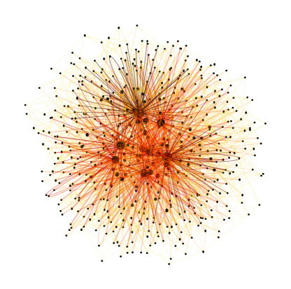
A typical network is shown in Fig. 1: While few nodes have many edges connecting them to other nodes, many nodes have few edges; the distribution of these following a power law. Although there have been several studies of Boolean variables on scale-free networks with social interaction networks in mind, most studies have focused on “friend” networks such as, for example, the Facebook com (a) network where person can “friend” person . Friendship can then be defined via a network edge between and with a positive weight. However, other networks exist where two persons and can either be “friends” or “foes” (i.e., a network with both positive- and negative-weight bonds). This appears, for example, in the slashdot network com (b) or when studying the robustness of opinion formation in, for example, an election process. The latter type of network is rarely studied, possibly due to the difficulties introduced by the negative-weighted edges in the system. However, they find wide applicability to many fields of science such as the aforementioned social networks, as well as other applications such as interaction networks between proteins or genes.
Why are Boolean problems on these scale-free networks interesting? Because they can be seen as the simplest model to study how general consensus forms on such a network for a decision problem with two possible outcomes. By placing Boolean variables on each node of the system, one can study either equilibrium or nonequilibrium properties of the thermodynamics of the Boolean variables and thus see how stable a given state of the system is. Generalizations to more complex decision problems can be readily accomplished by replacing the Boolean variables with, for example, -state Potts variables Yeomans (1992).
The entities interacting on a real network may have complex interactions, but models typically focus on connectivity in randomly occupied networks or on networks with uniform interactions between the entities. As illustrated above and as suggested in different studies Antall et al. (2006); Leskovec et al. (2010), many real networks possess both friend and foe interactions among the degrees of freedom. Because the network intrinsically has loops, this leads to frustration between the Boolean variables, quickly complicating the study of such systems.
Here, we study the critical behavior of the random-bond Ising model on scale-free networks. The model maps directly onto a friend or foe network (random bonds) with Boolean variables (Ising spins). Crucially, both ferromagnetic and antiferromagnetic interactions are allowed. Although many of the networks of experimental importance are dynamic and out-of-equilibrium, a thorough understanding of the equilibrium model provides a first step into the understanding of generic problems associated with networks with random interactions.
Monte Carlo simulations of Ising spins on scale-free networks and complex random graphs with uniform antiferromagnetic interactions Bartolozzi et al. (2006); Herrero (2009); Weigel and Johnston (2007) have shown that a stable spin-glass phase exists. Similarly, studies of a random-field ferromagnetic Ising model Imry and Ma (1975); Sethna et al. (1993) on scale-free graphs Lee et al. (2006) show that for the spins are always ordered (i.e., consensus is stable to local perturbations), whereas for a phase transition between a paramagnetic and ferromagnetic phase exists as a function of the random-field strength.
Surprisingly, for the case of a pure Ising spin glass defined on a scale-free graph no detailed numerical results exist with most results relying on analytical approximations and mean-field calculations Mooij and Kappen (2004); Kim et al. (2005); Ferreira et al. (2010); Ostilli et al. (2011). The detailed mean-field study by Kim et al. Kim et al. (2005) showed that for the critical temperature of the system diverges (i.e., the spins are stable to arbitrary local perturbations), whereas for a finite-temperature transition from a paramagnetic to a spin-glass state exists. In this work we improve on the results by Kim et al. by expanding the approach of Leone et al. Leone et al. (2002) for ferromagnetic systems to spin glasses. We present analytical results backed up by numerical results (using large-scale Monte Carlo simulations) for both Gaussian-distributed and bimodal edge weights between the Ising spins. We show that when the probability of positive (ferromagnetic) interactions and the probability for negative (antiferromagnetic) interactions is the same, the system undergoes a finite-temperature spin-glass transition if , in agreement with previous results Kim et al. (2005). However, when , a spin-glass (SG) phase is stable for all temperatures. Finally, in the cases where both spin-glass and ferromagnetic (FM) order would be expected (), only spin-glass order is present. Relating back to the social Gedankenexperiment, this would suggest that for certain networks the opinion of the individual is robust towards local perturbations and cannot be affected by global consensus.
In addition, we show that spin glasses on scale-free networks seem to obey universality. This means that, in the pure spin-glass case, the type of the interaction does not seem to affect the nature of the order when opinion forms. Furthermore, for Kim et al. (2005) spin glasses on scale-free networks have the same universality class as the mean-field Sherrington-Kirkpatrick Sherrington and Kirkpatrick (1975) Ising spin glass com (c).
In Sec. II we introduce the Hamiltonian studied, followed by how the networks are constructed in Sec. III. In Sec. IV we present analytical results and construct a – (network strength versus fraction of ferromagnetic bonds) phase diagram. Details about the simulations are shown in Sec. V, followed by numerical results in Sec. VI and concluding remarks.
II Model
The Hamiltonian of the Edwards-Anderson Ising spin glass Edwards and Anderson (1975); Binder and Young (1986) defined on a scale-free graph is given by
| (2) |
where the Ising spins lie on a scale-free graph with sites and interactions
| (3) |
In Eq. (3) if a bond is present between spin and and otherwise. denotes the mean connectivity of the underlying graph. The connectivity of site , , is sampled from the scale-free distribution, Eq. (1). The bond values are drawn from either a Gaussian distribution with zero mean and standard deviation unity, that is,
| (4) |
or a bimodal distribution defined via
| (5) |
In Sec. III we describe in detail how the scale-free graphs as shown in Fig. 1 are generated for the simulations.
III Generating scale-free graphs
One standard approach for the generation of scale-free networks is preferential attachment Barabasi and Albert (1999). In this physically inspired growth process, a new node is added to the graph at each step, and the probability of attaching to previously existing nodes depends on their edge degrees. This is believed to mimic the creation of scale-free networks in a wide variety of processes, where newcomers are more likely to associate with already-popular members of the network. The frustration that must be present for the disordered problem to be nontrivial requires that there be loops present in the network. The new nodes must therefore attach to multiple pre-existing nodes in this particular growth process. The simplest implementation of preferential attachment, where the probability of attaching to a node of edge degree is proportional to produces a power-law distribution of edge degrees with exponent . It is possible to modify the exponent, at least in the limit, by changing the function giving the probability of attachment Krapivsky et al. (2000); Krapivsky and Redner (2001).
Another technique for generating scale-free networks is to extend the classical “configuration model” Bender and Canfield (1978); Newman (2003); Catanzaro et al. (2005). Here, an edge degree distribution is chosen according to a power law of exponent and a graph is chosen randomly from the ensemble of all possible graphs consistent with the chosen edge degree distribution. The chosen graph is then fixed in time for a given sample (i.e., it is a quenched random graph). The procedure for generating the graphs starts by assigning stubs for each node, where is drawn from the distribution [Eq. (1)], and randomly pairing the stubs. These pairings make up the edges in the graph. If the resulting graph is valid (in our case, we do not allow double edges, and only connected graphs are considered), then it is accepted and may be used for simulation.
In practice, we use a slightly different approach which is much faster but is known to cause the selection of graphs to be slightly nonuniform Klein-Hennig and Hartmann (2011); com (d). If, during the pairing process, a connection is to be made between two stubs corresponding to the same node, this is not allowed. In the method described above, all edges are removed and the pairing starts from the beginning. Here, we simply reject the pairing and move on. This is not expected to affect our results significantly: The degree distribution is fixed independently of this method. In practice, the preferential attachment graphs are quite different than these random graphs, yet our tests give qualitatively similar results for the two cases. The results presented in this paper are from simulations using the quenched random graphs as defined above.
The graph-generation technique used in our simulations works for general degree distributions, although the acceptance rate may be prohibitively low for some graphs. For application to scale-free graphs, an upper bound is imposed on the allowed edge degrees, . Although we can generate graphs with exceeding , the ensemble is poorly defined in this case: Even randomly chosen graphs cannot be uncorrelated Burda and Krzywicki (2003); Boguñá et al. (2004); Catanzaro et al. (2005). We also set a lower bound on the edge degree . This eliminates spins which could be easily integrated out of the system and do not contribute to the frustration properties: dangling spins with only one attachment, and (possibly long) loops of spins which are not connected with any other spins.
IV Analytical results
Analytical results for spin glasses on scale-free networks were obtained previously Kim et al. (2005), and here we adapt a calculation for the Ising ferromagnet on a scale-free graph to the spin-glass case Leone et al. (2002).
IV.1 Replica approach
We use the replica approach and at first consider the disorder average of the replicated partition function for integer powers of
The double angular brackets denote an average only over the quenched interaction variables and . At the moment the connectivities are fixed. The constraints on these quantities, which are necessary to impose a scale-free degree distribution, will be introduced later [see Eq. (10)] as done byt the authors of Ref. Leone et al. (2002). In Eq. (IV.1) is a normalization constant and the inverse temperature. After an appropriate continuation to small values of the expression in Eq. (IV.1) is related to the free energy of the model via
| (7) |
Using a representation of the -function, the integrals in Eq. (IV.1) factorize resulting in
where is an Ising spin with components. The order parameters
| (9) |
and their conjugated fields allow one to perform the trace over the spin variables in Eq. (IV.1). After replacing the connectivity-dependent site averages with the appropriate averages over the degree distribution we obtain
| (10) | |||||
The partition function then acquires the form
| (11) |
with the trial free energy
where the average over the distribution is represented as . The integral in Eq. (11) can be evaluated with the method of steepest descent leading to a self-consistent equation for the order parameters :
| (13) |
Finding stable solutions to this equation in the limit would lead to the free energy of the model at all temperatures. This problem remains to be solved for general spin-glass Hamiltonians. However, here we are interested only in the transition temperature of the system. In this case the simplest replica symmetric analysis is sufficient.
IV.2 Replica-symmetric solution
Due to the Boolean nature of the Ising spins, the replica-symmetric solution of Eq. (13) only depends on the sum of the components of . The parametrization
| (14) |
allows one to perform the limit straightforwardly, which leads to the self-consistent equation for the local-field distribution
| (15) | |||||
with defined as
| (16) |
As pointed out in Ref. Leone et al. (2002) and calculated in Ref. Wemmenhove et al. (2005) this equation can be derived within the cavity framework Mézard and Parisi (2001). When connecting a new site to the system, one has to take into account the heterogeneity of the graph, which is reflected in the distribution on the right-hand side of Eq. (15). The spin-glass order parameter , where represents a thermal average, is related to the local-field distribution via
whereas the magnetization is given by
The expressions for the order parameters are derived by using real replicas of the system. Following the notation of Viana and Bray we also introduce the quantities
| (19) |
and remind the reader, that the inequality holds for all even .
The -function is always a solution of the self-consistent equation, Eq. (15). Due to the vanishing of all local fields, and consequently of the order parameters and , this solution intuitively corresponds to the paramagnetic phase. Based on physical grounds, we expect this solution to be unstable below a critical temperature, which thus signals a transition to a frozen low-temperature phase.
We first test the stability of this paramagnetic solution towards a spin-glass transition. To this end we introduce a distribution with a small on the right-hand side of Eq. (15). If the corresponding quantity of the resulting distribution on the left-hand side exceeds , the paramagnetic solution becomes unstable and the system undergoes a spin-glass transition. The critical temperature is given by the equation
| (20) |
To detect a transition towards a ferromagnetic phase a similar procedure using a distribution with a small can be applied. This leads to the stability criterion to determine , that is,
| (21) |
When lowering the temperature the system enters the frozen phase with the higher . Within the low-temperature phase no conjectures can be made from this “paramagnetic” analysis. Note that the usual procedure to determine (which relies on the moments of the distribution ) fails here for small values of the scale-free decay parameter (), because in this region the moments cease to exist.
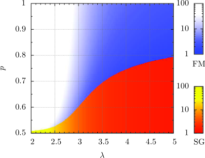
For a bimodal bond distribution [Eq. (5)] with minimum connectivity the solutions of Eqs. (20) and (21) are visualized in Fig. 2. The color represents the value of the critical temperature. The darker the color, the smaller the numerical value. Note that both transition temperatures diverge for , because the second moment of the degree distribution is infinite. In the blue-white region (top shaded region of the graph) the system is always ferromagnetic with increasing for . In the red-yellow region (bottom shaded region of the graph) the system is a spin glass at all finite temperatures with increasing for . For the particular case of for and finite for .
IV.3 Comparison to the static model
We briefly compare our result to previous calculations. In the work of Kim et al. Kim et al. (2005) the “static” model was used. In this approach a probability , is assigned to each vertex to obtain a scale-free graph with degree and mean connectivity . The results derived for the phase boundaries in Ref. Kim et al. (2005) rely on a truncation scheme which confines the number of the order parameters to the “most important” ones Viana and Bray (1985). At the replica-symmetric level, this approximation is equivalent to the assumption of Gaussian local fields, which can be avoided, using a variant of the approach described above.
Starting from Eq. (10) in Ref. Kim et al. (2005) we proceed using the order parameters
| (22) |
and their conjugated variables . The functions which still depend on the vertex weights can be transformed to integrals in the thermodynamic limit according to
In the last step we performed a substitution which directly leads to the scale-free distribution relevant for the static model
| (23) |
The partition function of the static model reduces to a saddle-point integral [see Eq. (11)] with a scale-free dependent part in the the trial free energy (IV.1):
Using the saddle-point equations and the replica-symmetric Ansatz, we obtain a self-consistent equation for the distribution of local fields
This equation is a generalization of the replica-symmetric equations for the Viana-Bray model Viana and Bray (1985); Monasson (1998) where the mean connectivity is sampled from the distribution . Moreover, the equation is similar to the self-consistent equation [Eq. (15)], where the connectivities are sampled from the distribution . This last approach is a generalization of the fixed-connectivity model to arbitrary degree distributions, and we prefer it due to its generality. The paramagnetic solution is a solution of Eq. (IV.3) which becomes unstable towards a spin-glass transition at the critical temperature
| (25) | |||||
The transition to a ferromagnetic phase occurs at the critical temperature
| (26) |
In the last line of Eq. (25) we performed the integrals which are convergent for only. This representation coincides with the predictions for the critical temperature in Ref. Kim et al. (2005). Here the results were obtained without resorting to a truncation scheme. Predictions for the de Almeida Thouless line de Almeida and Thouless (1978) relying on Gaussian approximations Cizeau and Bouchaud (1993) can lead to results which were shown to be wrong Neri et al. (2010); Janzen et al. (2010). The investigation of the phase boundaries in the presence of an external magnetic field seems promising in this approach, and will be reported elsewhere.
IV.4 Critical exponents
We now turn to the computation of the critical exponent which governs the growth of the order parameter close to the transition temperature. The order parameter is proportional to , here is the reduced temperature (i.e., and a critical exponent).
Note that close to all are small, as is close to a function. This allows us to neglect with large in this region while keeping the dominant terms (i.e., for the spin-glass transition and for the ferromagnetic transition). In particular, close to the order parameters and are proportional to and , respectively. It is therefore sufficient to investigate how these quantities evolve from zero below .
We start with the spin-glass transition and derive a self-consistent equation for :
| (27) |
where are Taylor coefficients of . To obtain Eq. (27) we use the self-consistent equation [Eq. (15)] for and employ a series expansion in terms of the . We then evaluate all averages with respect to and and finally perform the aforementioned approximation (i.e., neglect all with ).
If we recover the Sherrington-Kirkpatrick mean-field critical exponents by truncating the second sum after the contribution on the right hand side of the equation, which amounts to
that is,
| (28) |
For the average in the denominator of the last equation diverges and the usual technique to extract the critical exponent does not work.
For we note that due to the combinatorial factor in Eq. (27) the lower (important) powers of have a prefactor proportional to , such that the divergent part () depends on the combination only. We assume that this is the important dependence and introduce a function in the following way:
In the last line we scaled out by a substitution leading to the lower integration bound . The quadratic dependence of at the origin due to the fact that the series expansion starts with allows one to put for . Inserting the above steps into Eq. (27) we obtain
This means
| (29) |
which agrees with the result of Kim et al. Kim et al. (2005) derived within the static approximation. The limiting case needs some special care, leading to logarithmic corrections [i.e., ].
To reproduce the results for the critical exponent in the ferromagnetic sector, which were calculated by the authors of Ref. Leone et al. (2002), the same technique can be used. In particular
| (30) |
This means the system is in the mean-field universality class for because, within
For we face the same problem as in the spin-glass sector when , because the average in the denominator diverges. Performing analogous considerations leads to
| (31) |
Finally, for , .
Summarizing, for [] in the SG [FM] sector, the critical exponents agree with the mean-field case, whereas for [] in the SG [FM] sector the critical exponents depend on the exponent .
V Numerical details
We validate the aforementioned analytical results using Monte Carlo simulations. In particular, the numerical results show the strength of the different corrections to scaling depending on the choice of the exponent of the scale-free network.
V.1 Observables
To determine the location of both the ferromagnetic and spin-glass phase transitions we measure first the Binder cumulant Binder (1981) defined via
| (32) |
In Eq. (32), represents an average over the disorder via , the random graphs via , and Monte Carlo time (i.e., ). Furthermore, is either the magnetization in the ferromagnetic sector defined via
| (33) |
or the spin-glass overlap in the spin-glass sector given by
| (34) |
In Eq. (34), “” and “” represent two copies of the system with the same disorder. The Binder ratio is dimensionless and thus has the simple scaling form
| (35) |
where represents the transition temperature. The expression in Eq. (35) is valid in the non-mean-field region (i.e., for in the spin-glass sector and in the ferromagnetic sector Kim et al. (2005)). In the spin-glass mean-field region () Eq. (35) is replaced by Larson et al. (2010)
| (36) |
Note that the two-point finite-size correlation length Cooper et al. (1982); Palassini and Caracciolo (1999); Ballesteros et al. (2000); Martín-Mayor et al. (2002) typically used to pinpoint transitions in glassy systems cannot be used here because the spins are placed on a lattice that has no geometry.
The calculation of the Binder ratio allows one to determine and the critical exponent for both the spin-glass and ferromagnetic sectors. However, to fully characterize the critical behavior of the model, a second critical exponent has to be computed Yeomans (1992). We have also computed the susceptibility given by
| (37) |
In the ferromagnetic case we therefore measure
| (38) |
with the magnetization given by Eq. (33), whereas in the spin-glass case we measure
| (39) |
with the spin-glass overlap defined in Eq. (34). In general, the scaling behavior of the susceptibility is given by
| (40) |
where a simple finite-size scaling yields the exponent . Unfortunately, fluctuations in the data are huge and thus the determination of the critical exponent is not possible. However, in the mean-field regime, the finite-size scaling form presented in Eq. (40) is replaced by
| (41) |
Therefore, curves of should have the same scaling behavior as the Binder ratio [Eq.(36)]: When data for different system sizes cross at a point (up to scaling corrections).
V.2 Equilibration and simulation parameters
The simulations are done using the parallel tempering Monte Carlo method Hukushima and Nemoto (1996). For the pure spin glass we first simulate the system with Gaussian disorder to obtain an idea of the equilibration behavior when the Ising model with disorder is defined on a scale-free graph. Furthermore, in the Gaussian case we can perform a rigorous equilibration test Katzgraber et al. (2001, 2009) where the energy per spin [ with defined in Eq. (2)] is compared to an expression derived from the link overlap [defined below in Eq. (42)]. The data for both the energy per spin and the energy per spin computed from the link overlap,
| (42) |
where
| (43) |
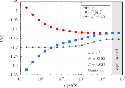
have to coincide when the system is in thermal equilibrium. In Eqs. (42) and (43) is the number of nonzero bonds of a given sample. Note that the expression in Eq. (42) is valid for the spin-glass sector, however, it represents a conservative bound for the ferromagnetic sector Katzgraber et al. (2001). Furthermore, is inside the disorder average because the number of bonds fluctuates from sample to sample. Sample data are shown in Fig. 3. Once the data for the squared order parameter (shifted for better viewing in Fig. 3) are also in thermal equilibrium.
For the bimodal disorder distribution and the ferromagnetic sector the aforementioned equilibration test cannot be used. In this case we preform a logarithmic binning of all observables. Once the data for the last three bins agree within error bars we deem the system to be in thermal equilibrium. The simulation parameters are shown in Table 1.
| Gauss | |||||||
|---|---|---|---|---|---|---|---|
| Gauss | |||||||
| Gauss | |||||||
| Gauss | |||||||
| Gauss | |||||||
| Gauss | |||||||
| Gauss | |||||||
| Gauss | |||||||
| Gauss | |||||||
| Gauss | |||||||
| Gauss | |||||||
| Gauss |
VI Numerical results
We first study Gaussian disorder where we have a strong equilibration test to ensure that the data are in thermal equilibrium. Corrections to scaling are very large for this model despite the large number of samples studied.
VI.1 Gaussian disorder
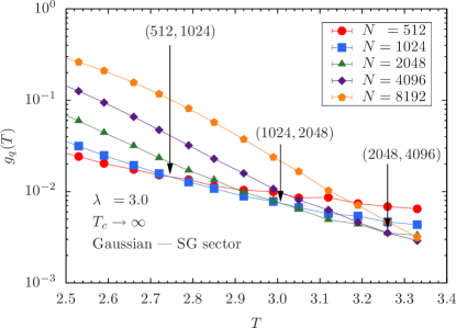
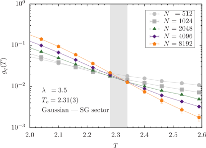
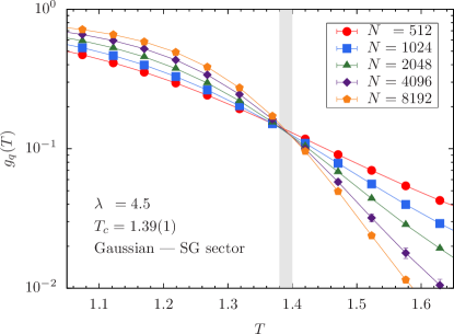
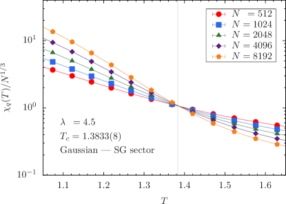
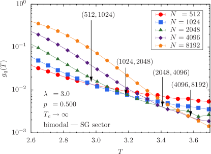
Figure 4 shows data for the Binder ratio for Gaussian disorder and , right at the onset (see Fig. 2) where the critical temperature for the spin-glass (SG) sector starts to diverge. The crossing temperatures between lines for / pairs grow with the system size in agreement with the analytic calculations. To prevent for the SG sector to diverge, the bonds would have to be re-scaled. Furthermore, there is no transition in the ferromagnetic sector (not shown), in agreement with the analytical calculations.
In Fig. 5 we show data for . In agreement with the analytical predictions is finite, albeit with huge corrections to scaling. We estimate . Note that this estimate is computed via a finite-size scaling of the data and only takes statistical fluctuations into account. We have no control over finite-size corrections. A crude extrapolation suggests that the critical temperature will likely be larger than the quoted analytical value which we treat as a lower bound. This is a generic problem for the estimates of the critical temperature made in the spin-glass sector. Again, there is no transition in the ferromagnetic sector.
Finally, Fig. 6 shows data for . The top panel shows the Binder ratio as a function of temperature. The data cross at . Using Eq. (36) [i.e., fixing “” in Eq. (35)] we obtain , which agrees within error bars with the previous estimate. This result is verified by data on the scaled spin-glass susceptibility (bottom panel of Fig. 6) where the data also cross in the same region. A finite-size scaling analysis of gives , a value of higher precision than when using the Binder ratio. For all values of studied where the estimates for the critical exponent are listed in Table 2. Note that for , “” in the scaling form. However, we have allowed for the value to fluctuate when estimating as well.
VI.2 Bimodal disorder
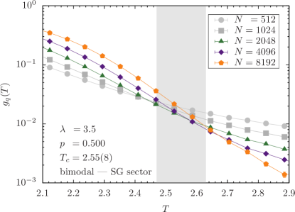
Figure 7 shows data for the Binder ratio for bimodal disorder with and . The chosen value of is right at the onset (see Fig. 2) where the critical temperature for the spin-glass SG starts to diverge. As for the Gaussian case presented in Sec. VI.1, crossing points between lines for / pairs grow with the system size in agreement with the analytic calculations (i.e., ). Furthermore, for the FM sector there is no transition (not shown).
In Fig. 8 we show data for and . In agreement with the analytical predictions is finite, albeit with large corrections to scaling. We estimate . Again, there is no ferromagnetic transition (not shown).
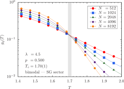
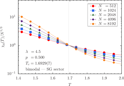
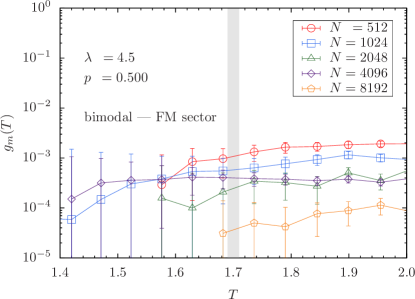
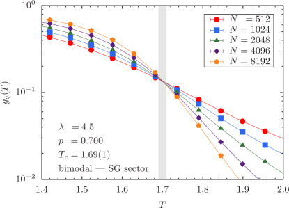
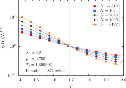
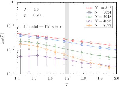
We now study in detail for different concentrations of ferromagnetic bonds . Figure 9 shows data for the Binder ratio for and for both SG and FM sectors. For the SG sector (top panel), the data cross cleanly at [ when Eq. (36) is used]. The center panel shows data for the scaled spin-glass susceptibility. We obtain , in agreement with the estimate from the Binder ratio, albeit with higher precision. However, for the FM sector (bottom panel) the data strongly suggest that is not defined, in agreement with the analytic predictions. For the phase boundary between the FM and the SG sector lies somewhere between and , see Fig. 2. Therefore, we expect that for we only have SG order, whereas for the system orders ferromagnetically.
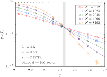
The case for is shown in Fig. 10. Like for , the data for the SG sector show a clear transition, whereas the data for the FM sector suggest that there is no transition. Note that the estimates for agree within error bars with the estimates for , suggesting that the phase diagram does not depend on in the SG regime, in agreement with the analytical calculations. For there is no SG order (not shown, in agreement with the analytical results). Moreover, , see Fig. 11.
VI.3 Universality?
To determine if two systems share the same universality class two independent critical exponents need to be computed. However, fluctuations in the data are large and therefore estimating the critical exponent from a finite-size scaling analysis of the susceptibility is difficult. Even worse, is not properly defined for mean-field models and only , , and are available.
As shown above in Sec. IV, as well as the work of Kim et al. Kim et al. (2005) and Dorogovtsev et al. Dorogovtsev et al. (2008), the critical exponents for spin glasses and ferromagnets on scale-free graphs depend on the exponent . In particular, for the spin-glass sector is predicted to share the same universality class as the mean-field Sherrington-Kirkpatrick model. For one can show that for the critical exponent one finds . Similar predictions exist for the ferromagnetic sector where mean-field behavior is recovered for . However, it remains to be determined if the type of disorder (e.g., Gaussian or bimodal) might change the critical exponents.
We compute the critical exponents in an unbiased fashion and with a statistical error bar by letting and be parameters. Close to the transition temperature the scaling function can be represented by a third-order polynomial. This is typically a very good approximation. If the optimal values of the critical parameters and are chosen, then data for different system sizes should collapse onto a single curve, the scaling function. Therefore, by searching for the optimal fit to a third-order polynomial while minimizing the chi-square of the fit with respect to the critical parameters allows us to determine their optimal values. Statistical error bars to the optimal values are determined by a bootstrap analysis. Note that these error bars take statistical fluctuations into account but cannot properly account for systematic deviations due to corrections to scaling com (e).
| — | — | — | — | |||
| — | — | |||||
| — | — | |||||
| fixed | — | — | ||||
| — | — | — | — | |||
| — | — | |||||
| fixed | — | — | ||||
| — | — | — | — | |||
| — | — | — | ||||
| Gauss | — | — | — | — | ||
| Gauss | — | — | ||||
| Gauss | — | — | ||||
| Gauss | fixed | — | — | |||
| Gauss | — | — | — | — |
To test for universality we estimate the critical exponent and the value of the dimensionless Binder ratio at Katzgraber et al. (2006) (see Table 2). Because fluctuations in are very large and is not properly defined for () in the spin-glass (ferromagnetic) sector we compare in detail in the spin-glass sector. For , , which agrees within error bars with . For , , which agrees within error bars with . In the bimodal case, we find also that agrees within error bars with , thus suggesting the the same universality class might be shared below the spin-glass–to–ferromagnet phase boundary for all values of . The mean-field Viana-Bray model Viana and Bray (1985) resembles a fixed-connectivity random graph and is in the same universality class as the Sherrington-Kirkpatrick model. Recent simulations Wittmann and Young (2012) have shown that for the mean-field universality class , in agreement with our results for .
Summarizing, our results suggest that for a given value of the networks with both Gaussian and bimodal disorder share the same universality class. In addition, for values of the spin-glass sector shares the same universality class as the mean-field Sherrington-Kirkpatrick model.
VII Conclusions
We have studied Boolean (Ising) variables on a scale-free graph with competing interactions. Our analytical and numerical results show that for the critical temperature diverges with the system size. For larger values of the system undergoes a finite-temperature transition between a spin-glass and a paramagnetic phase. The robustness of both the ferromagnetic and spin-glass phases suggest that Boolean decision problems on scale-free networks are quite stable to local (temperature) perturbations. For the case with bimodal disorder, we show that for a large enough fraction of ferromagnetic bonds the system orders ferromagnetically at finite temperatures. Finally, for a given value of universal critical parameters for both Gaussian and bimodal disorder agree, suggesting universal behavior.
Real networks typically have exponents . It would be interesting to study such a network in the future. Furthermore, the effect of “global biases” (field terms) will also be studied. Finally, opinion formation is an intrinsically nonequilibrium process. For example, what are the temporal patterns of the agents on the networks? What are the effects of time-dependent interactions?
Acknowledgements.
We would like to thank Alexander K. Hartmann, M. Niemann, M. Schechter, M. Wittmann and A. P. Young for fruitful discussions. We also thank R. S. Andrist for assistance. H.G.K. acknowledges support from the SNF (Grant No. PP002-114713) and the NSF (Grant No. DMR-1151387). We would like to thank the Texas Advanced Computing Center (TACC) at The University of Texas at Austin for providing HPC resources (Ranger Sun Constellation Linux Cluster), ETH Zurich for CPU time on the Brutus cluster, and Texas A&M University for access to their eos and lonestar clusters.References
- Albert et al. (1999) R. Albert, H. Jeong, and A.-L. Barabási, Internet: Diameter of the World-Wide Web, Nature 401, 130 (1999).
- Albert and Barabási (2002) R. Albert and A.-L. Barabási, Statistical mechanics of complex networks, Rev. Mod. Phys. 74, 47 (2002).
- com (a) http://facebook.com.
- com (b) http://slashdot.org.
- Yeomans (1992) J. M. Yeomans, Statistical Mechanics of Phase Transitions (Oxford University Press, Oxford, 1992).
- Antall et al. (2006) T. Antall, P. L. Krapivsky, and S. Redner, Social balance on networks: The dynamics of friendship and enmity, Physica D 224, 130 (2006).
- Leskovec et al. (2010) J. Leskovec, D. Huttenlocher, and J. Kleinberg, in Proceedings of the 28th ACM Conference on Human Factors in Computing Systems (2010), p. 1361.
- Bartolozzi et al. (2006) M. Bartolozzi, T. Surungan, D. B. Leinweber, and A. G. Williams, Spin-glass behavior of the antiferromagnetic Ising model on a scale-free network, Phys. Rev. B 73, 224419 (2006).
- Herrero (2009) C. P. Herrero, Antiferromagnetic Ising model in scale-free networks, Eur. Phys. J. B 70, 435 (2009).
- Weigel and Johnston (2007) M. Weigel and D. Johnston, Frustration effects in antiferromagnets on planar random graphs, Phys. Rev. B 76, 054408 (2007).
- Imry and Ma (1975) Y. Imry and S.-K. Ma, Random-Field Instability of the Ordered State of Continuous Symmetry, Phys. Rev. Lett. 35, 1399 (1975).
- Sethna et al. (1993) J. P. Sethna, K. Dahmen, S. Kartha, J. A. Krumhansl, B. W. Roberts, and J. D. Shore, Hysteresis and hierarchies: Dynamics of disorder-driven first-order phase transformations, Phys. Rev. Lett. 70, 3347 (1993).
- Lee et al. (2006) S. H. Lee, H. Jeong, and J. D. Noh, Random field Ising model on networks with inhomogeneous connections, Phys. Rev. E 74, 031118 (2006).
- Mooij and Kappen (2004) J. M. Mooij and H. J. Kappen, Spin-glass phase transitions on real-world graphs (2004), (arXiv:cond-mat/0408378).
- Kim et al. (2005) D.-H. Kim, G. J. Rodgers, B. Kahng, and D. Kim, Spin-glass phase transition on scale-free networks, Phys. Rev. E 71, 056115 (2005).
- Ferreira et al. (2010) A. L. Ferreira, J. F. F. Mendes, and M. Ostilli, First- and second-order phase transitions in Ising models on small-world networks: Simulations and comparison with an effective field theory, Phys. Rev. E 82, 011141 (2010).
- Ostilli et al. (2011) M. Ostilli, A. L. Ferreira, and J. F. F. Mendes, Critical behavior and correlations on scale-free small-world networks: Application to network design, Phys. Rev. E 83, 061149 (2011).
- Leone et al. (2002) M. Leone, A. Vázquez, A. Vespignani, and R. Zecchina, Ferromagnetic ordering in graphs with arbitrary degree distribution, Eur. Phys. J. B 28, 191 (2002).
- Sherrington and Kirkpatrick (1975) D. Sherrington and S. Kirkpatrick, Solvable model of a spin glass, Phys. Rev. Lett. 35, 1792 (1975).
- com (c) Note that similar behavior is found in the ferromagnetic sector where the change to the mean-field Ising universality class occurs at Dorogovtsev et al. (2008).
- Edwards and Anderson (1975) S. F. Edwards and P. W. Anderson, Theory of spin glasses, J. Phys. F: Met. Phys. 5, 965 (1975).
- Binder and Young (1986) K. Binder and A. P. Young, Spin glasses: Experimental facts, theoretical concepts and open questions, Rev. Mod. Phys. 58, 801 (1986).
- Barabasi and Albert (1999) A. L. Barabasi and R. Albert, Science 286, 509 (1999).
- Krapivsky et al. (2000) P. L. Krapivsky, S. Redner, and F. Leyvraz, Connectivity of growing random networks, Phys. Rev. Lett. 85, 4629 (2000).
- Krapivsky and Redner (2001) P. L. Krapivsky and S. Redner, Organization of growing random networks, Phys. Rev. E 63, 066123 (2001).
- Bender and Canfield (1978) E. A. Bender and E. R. Canfield, The asymptotic number of labeled graphs with given degree sequences, J. Comb. Theory A 24, 296 (1978).
- Newman (2003) M. E. J. Newman, in Handbook of Graphs and Networks, edited by S. Bornholdt and H. G. Schuster (Wiley-VCH, Berlin, 2003).
- Catanzaro et al. (2005) M. Catanzaro, M. Boguñá, and R. Pastor-Satorras, Generation of uncorrelated random scale-free networks, Phys. Rev. E 71, 027103 (2005).
- Klein-Hennig and Hartmann (2011) H. Klein-Hennig and A. K. Hartmann, Bias in generation of random graphs (2011), (arxiv:cond-mat/1107.5734).
- com (d) Note that the method we use to generate the scale-free graphs also suffers from the bias recently characterized by the authors of Ref. Klein-Hennig and Hartmann (2011). However, for , which are the values we are interested in, this has no effect on the data.
- Burda and Krzywicki (2003) Z. Burda and A. Krzywicki, Uncorrelated random networks, Phys. Rev. E 67, 046118 (2003).
- Boguñá et al. (2004) M. Boguñá, R. Pastor-Satorras, and A. Vespignani, Cut-offs and finite size effects in scale-free networks, Eur. Phys. J. B 38, 205 (2004).
- Wemmenhove et al. (2005) B. Wemmenhove, T. Nikoletopoulos, and J. P. L. Hatchett, Replica symmetry breaking in the ’small world’ spin glass, J. Stat. Mech. P11007 (2005).
- Mézard and Parisi (2001) M. Mézard and G. Parisi, The Bethe lattice spin glass revisited, Eur. Phys. J. B 20, 217 (2001).
- Viana and Bray (1985) L. Viana and A. J. Bray, Phase diagrams for dilute spin glasses, J. Phys. C 18, 3037 (1985).
- Monasson (1998) R. Monasson, Optimization problems and replica symmetry breaking in finite connectivity spin glasses, J. Phys. A 31, 513 (1998).
- de Almeida and Thouless (1978) J. R. L. de Almeida and D. J. Thouless, Stability of the Sherrington-Kirkpatrick solution of a spin glass model, J. Phys. A 11, 983 (1978).
- Cizeau and Bouchaud (1993) P. Cizeau and J. P. Bouchaud, Mean field theory of dilute spin-glasses with power-law interactions, J. Phys. A 26, L187 (1993).
- Neri et al. (2010) I. Neri, F. L. Metz, and D. Bollé, The phase diagram of Lévy spin glasses, J. Stat. Mech. P01010 (2010).
- Janzen et al. (2010) K. Janzen, A. Engel, and M. Mézard, Thermodynamics of the Lévy spin glass, Phys. Rev. E 82, 021127 (2010).
- Binder (1981) K. Binder, Critical properties from Monte Carlo coarse graining and renormalization, Phys. Rev. Lett. 47, 693 (1981).
- Larson et al. (2010) D. Larson, H. G. Katzgraber, M. A. Moore, and A. P. Young, Numerical studies of a one-dimensional 3-spin spin-glass model with long-range interactions, Phys. Rev. B 81, 064415 (2010).
- Cooper et al. (1982) F. Cooper, B. Freedman, and D. Preston, Solving theory with Monte Carlo, Nucl. Phys. B 210, 210 (1982).
- Palassini and Caracciolo (1999) M. Palassini and S. Caracciolo, Universal Finite-Size Scaling Functions in the 3D Ising Spin Glass, Phys. Rev. Lett. 82, 5128 (1999).
- Ballesteros et al. (2000) H. G. Ballesteros, A. Cruz, L. A. Fernandez, V. Martin-Mayor, J. Pech, J. J. Ruiz-Lorenzo, A. Tarancon, P. Tellez, C. L. Ullod, and C. Ungil, Critical behavior of the three-dimensional Ising spin glass, Phys. Rev. B 62, 14237 (2000).
- Martín-Mayor et al. (2002) V. Martín-Mayor, A. Pelissetto, and E. Vicari, Critical structure factor in Ising systems, Phys. Rev. E 66, 026112 (2002).
- Hukushima and Nemoto (1996) K. Hukushima and K. Nemoto, Exchange Monte Carlo method and application to spin glass simulations, J. Phys. Soc. Jpn. 65, 1604 (1996).
- Katzgraber et al. (2001) H. G. Katzgraber, M. Palassini, and A. P. Young, Monte Carlo simulations of spin glasses at low temperatures, Phys. Rev. B 63, 184422 (2001).
- Katzgraber et al. (2009) H. G. Katzgraber, D. Larson, and A. P. Young, Study of the de Almeida-Thouless line using power-law diluted one-dimensional Ising spin glasses, Phys. Rev. Lett. 102, 177205 (2009).
- Dorogovtsev et al. (2008) S. N. Dorogovtsev, A. V. Goltsev, and J. F. F. Mendes, Critical phenomena in complex networks, Rev. Mod. Phys. 80, 1275 (2008).
- com (e) Note that all our numerical estimates for the critical temperatures are approximately 5% above the analytically-determined values. Further studies would be needed to better understand this small deviation. The small systematic deviation could be, for example, attributed to corrections to scaling or the fact that the analytical results take all graphs to be equally weighted, whereas this is not the case in the numerical results. However, we emphasize that the agreement is remarkably good.
- Katzgraber et al. (2006) H. G. Katzgraber, M. Körner, and A. P. Young, Universality in three-dimensional Ising spin glasses: A Monte Carlo study, Phys. Rev. B 73, 224432 (2006).
- Wittmann and Young (2012) M. Wittmann and A. P. Young, Spin glasses in the nonextensive regime, Phys. Rev. E 85, 041104 (2012).