Blind Null-Space Learning for MIMO Underlay Cognitive Radio Networks

Abstract

This paper proposes a blind technique for MIMO cognitive radio Secondary Users (SU) to transmit in the same band simultaneously with a Primary User (PU) under a maximum interference constraint. In the proposed technique, the SU is able to meet the interference constraint of the PU without explicitly estimating the interference channel matrix to the PU and without burdening the PU with any interaction with the SU. The only condition required of the PU is that for a short time interval it uses a power control scheme such that its transmitted power is a monotonic function of the interference inflicted by the SU. During this time interval, the SU iteratively modifies the spatial orientation of its transmitted signal and measures the effect of this modification on the PU’s total transmit power. The entire process is based on energy measurements which is very desirable from an implementation point of view.

I Introduction

The emergence of Multiple Input Multiple Output (MIMO) communication opens new directions and possibilities for Cognitive Radio (CR) networks [ZhangExploiting2008, ScutariCognitive2008, ScutariMIMO2010]. In particular, in underlay CR networks, MIMO technology enables the SU to transmit a significant amount of power simultaneously in the same band with the PU without interfering with him if the SU utilizes separate spatial dimensions than the PU. This spatial separation requires that the interference channel from the SU to the PU be known to the SU. Thus, acquiring this knowledge, or operating without it, is a major issue of active research [HuangDecentralized2011, ZhangRobust2009, ZhangOptimal2011, ChenInterference2011, YiNullspace]. We consider MIMO primary and secondary systems defined as follows: we assume a flat-fading MIMO channel with one primary and multiple SUs. Let ${\bf H}_{1j}\in$ ${\mathbb{C}}^{n_{1}\times n_{j}}$ be the channel matrix between user $j$’s transmitter and the PU’s receiver. In the underlay CR paradigm, SUs are constrained not to exceed a maximum interference level at the PU, i.e.

$$\|{\bf{H}}_{1j}{\bf{x}}_{j}(t)\|^{2}\leq\eta,~{}\forall j\neq 1,$$ (1)

where ${\bf{x}}_{j}$ is SU $j$’s ($j>1$) transmit signal and $\eta>0$ is the maximum interference constraint. If $\eta=0$, the SUs are strictly constrained to transmit only within the null space of the matrix ${\bf{H}}_{1j}$.

The optimal power allocation for the case of a single SU who knows the matrix ${\bf{H}}_{21}$ in addition to its own Channel State Information (CSI) was derived by Zahng and Liang [ZhangExploiting2008]. For the case of multiple SUs, Scutari at al. [ScutariMIMO2010] formulated a competitive game between the secondary users. Assuming that the interference matrix to the PU is known by each SU, they derived conditions for the existence and uniqueness of a Nash Equilibrium point to the game. Zhang et al. [ZhangRobust2009] were the first to take into consideration the fact that the interference matrix ${\bf{H}}_{12}$ may not be perfectly known (but is partially known) to the SU. They proposed Robust Beamforming to assure compliance with the interference constraint of the PU while maximizing the SU’s throughput. Other work for the case of an unknown interference channel with known probability distribution is due to Zhang and So [ZhangOptimal2011], who optimized the SU throughput under a constraint on the maximum probability that the interference to the PU is above a threshold.

The underlay concept of CR in general and MIMO CR in particular is that the SU must be able to mitigate the interference to the PU blindly without any cooperation. Yi [YiNullspace] proposed a solution in the case where the SU learns the channel matrix based on channel reciprocity between the PU where the SU listens to the PU transmitted signal and estimates ${\bf{H}}_{12}$’s null space from the signal’s second order statistics. This work was enhanced by Chen et. al. [ChenInterference2011]. Both works requires channel reciprocity and therefore are restricted to a PU that uses Time Division Duplexing (TDD). Once the SU obtains the null space of ${\bf{H}}_{12}$, it does not interfere with the PU as long as his signal occupies that null space.

Other than in the channel reciprocity case, obtaining the value of ${\bf{H}}_{1j}$ by the SUs (i.e. the interference channel to the PU) requires cooperation from the PU in the estimation phase, e.g. where the SU transmits a training sequence, from which the PU estimates ${\bf{H}}_{1j}$ and feeds it back to the SU. Cooperation of this nature increases system complexity overhead, since it requires a handshake between both systems and in addition, the PU needs to be synchronized to the SU’s training sequence. This is one of the major technical obstacles that prevents underlay CRs from being widespread.

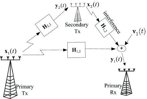
The objective of this work is to design a simple procedure such that MIMO underlay SU can meet the interference constraint to the PU without explicitly estimating the matrix ${\bf{H}}_{1j}$ and without burdening the PU with any handshaking, estimation or synchronization associated with the SUs. In the proposed scheme (see Fig. 1) the PU is not cooperating at all with the SU and operates as if it is the only system in the medium (as current PUs operate today). The only condition required is that for some short time interval (that may be much shorter than the entire learning process), the PU will be using a power control scheme such that its transmitted power is a monotonic function of the interference inflicted by the SU. Under this condition, we propose a learning algorithm in which the SU is gradually reducing the interference to the PU by iteratively modifying the spatial orientation of its transmitted signal and measuring the effect of this modification on the PU’s total transmit power. The entire process is based on energy measurements and on detecting energy variations. Therefore, it does not require any handshake or synchronization between the PU and the SU.

The paper is organized as follows: Section II provides the system description and some notation. Section III presents a blind approach for realizing the Cyclic Jacobi technique for calculating the Eigenvalue Decomposition (EVD) of an unobserved matrix; this will be the building block of the blind null space learning algorithm presented in Section LABEL:Section:BNSL_Algorithm and analyzed in Section LABEL:Complexity_and_Convergence. Simulations and Conclusions are presented in Sections LABEL:Section:Simulation and LABEL:Section:coclusions, respectively.

Figure 1: The addressed cognitive radio scheme. The matrix ${\bf{H}}_{1,2}$ is unknown to the secondary transmitter and ${\bf{v}}_{1}$ (t) is a stationary noise (which may include stationary interference). The interference from the SU, ${\bf H}_{12}{\bf{x}}_{2}(t)$, is treated as noise, i.e. no interference cancellation is performed. The SU measures the energy variations in ${\bf{y}}_{2}(t)$ according to which it varies its transmission scheme until the interference to the PU becomes sufficiently small such that it does not affect ${\bf{y}}_{2}(t)$.

II Problem Formulation

Consider a flat fading MIMO interference channel with a single PU and a single SU without interference cancellation, i.e. each system treats the other system’s signal as noise. The PU’s received signal is given by

$${\bf{y}}_{1}(t)={\bf{H}}_{11}{\bf{x}}_{1}(t)+{\bf{H}}_{12}{\bf{x}}_{2}(t)+{\bf{v}}_{1}(t),\;t\in{\mathbb{N}}$$ (2)

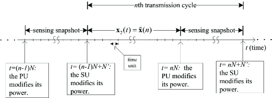
where ${\bf{v}}_{1}(t)$ is a zero mean stationary noise. In this paper all vectors are column vectors. Let ${\bf{A}}$ be an $l\times m$ complex matrix, then, its null space is defined as ${\cal N}({\bf{A}})=\{{\bf{y}}\in\mathbb{C}^{m}:{\bf{A}}{\bf{y}}={\mathbf{0}}\}$ where ${\mathbf{0}}=[0,...,0]^{\rm T}$. For simplicity ${\bf{H}}_{12}$ will be denoted by ${\bf{H}}$ and the matrix ${\bf{H}}^{*}{\bf{H}}$ will be denoted by ${\bf{G}}$. The time line $\mathbb{N}$ will be divided into $N$-length intervals referred to as transmission cycles where, for each cycle, the SU’s signal will be constant (this is required only during the learning process), i.e.

$$\begin{array}[]{lll}{\bf{x}}_{2}((n-1)N+N^{\prime})={\bf{x}}_{2}((n-1)N+1)\\ ~{}~{}~{}~{}~{}~{}~{}~{}~{}~{}~{}~{}=\cdots={\bf{x}}_{2}(Nn+N^{\prime}-1)\triangleq\tilde{\bf{x}}(n),\end{array}$$ (3)

where the time interval $nN<t\leq nN+N^{\prime}-1$ ($N^{\prime}<<N$) is the snapshot in which the SU measures a function

$$q(n)=\frac{1}{N^{\prime}}\sum_{t=Nn}^{Nn+N^{\prime}-1}\|{\bf{y}}_{2}(t)\|^{2}$$ (4)

where ${\bf y}_{2}$ is the observed signal at the secondary transmitter that includes the primary system’s transmitted signal (see Figure 1). The SU’s objective is to learn ${\cal N}({\bf{H}})$ from $\{\tilde{\bf{x}}(n),q(n)\}_{n\in{\mathbb{N}}}$. This learning process is carried out in learning stages where each stage consists of $K$ transmission cycles. We will index each learning stage by $k$. The indexing method is depicted in Figure 2.

Figure 2: The time indexing that is used in this paper. $t$ indexes the basic time unit (pulse time) where $N$ time units constitute a transmission cycle that is indexed by $n$. Furthermore, $K$ transmission cycles constitute a learning phase (this is not illustrated in this figure).

During the learning process, the SU varies the interference to the PU by transmitting a different interfering signal $\tilde{\bf{x}}(n)$. The secondary transmitter measures ${\bf{y}}_{2}(t)$ from which it extracts $q(n)$ in order to monitor the PU’s transmitted power, i.e. $\frac{1}{N^{\prime}}\sum_{t=nN}^{Nn+N^{\prime}-1}\|{\bf{x}}_{1}(t)\|^{2}$. Each transmission cycle, $N$, corresponds to the PU’s power control cycle, i.e. to the time interval between two consecutive power adaptations made by the PU. In fact the actual $q(n)$ is not important as long as it satisfies the following condition.

Assumption 1

Let $k\in{\mathbb{N}}$, then for every $K(k-1)\leq n<kK$ the function $q(n)$ satisfies $q(n)=f_{k}(\|{\bf{H}}\tilde{\bf{x}}(n)\|^{2})$ where $f_{k}:{\mathbb{R}_{+}}\rightarrow{\mathbb{R}_{+}}$ is a sequence of strictly monotonous continuous increasing (decreasing) functions.

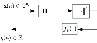
Without loss of generality, we assume that $f_{k}$ is a sequence of monotone increasing functions. The most important trait (that will be used in this paper) that follows from Assumption 1 is that for every $K(k-1)\leq n,m<kK$, $f_{k}(\|{\bf{H}}\tilde{\bf{x}}(n)\|^{2})\geq f_{k}(\|{\bf{H}}\tilde{\bf{x}}(m)\|^{2})$ implies that $\|{\bf{H}}\tilde{\bf{x}}(n)\|^{2}\geq\|{\bf{H}}\tilde{\bf{x}}(m)\|^{2}$. The problem is illustrated in Figure 3. From a system point of view, Assumption 1 means that between two consecutive transmission cycles the primary transmitter’s power can be modified only due to variations in the interference level from the SU that is at the learning process and not in a steady state.

In the following we provide an example for conditions under which Assumption 1 is satisfied. To simplify the exposition, we replace the function $q$ in (4) with

$$q(n)=\frac{1}{N^{\prime}}\sum_{t=nN}^{Nn+N^{\prime}-1}{\rm{E}}\{\|{\bf{y}}_{2}(t)\|^{2}\}$$ (5)

In doing so, we ignore the measurement noise at the secondary transmitter. Such $q(n)$ satisfies Assumption 1 if for example

1. The PU’s signal has the following form: ${\bf x}_{1}(t)=\sqrt{p_{1}(n)}{\bf P}_{1}{\bf s(t)}$ where ${\bf P}_{1}$ is a constant pre-coding matrix, $\text{E}\left\{\mathbf{s}(t)\mathbf{s}{}^{*}(t)\right\}=\mathbf{I}$, and $p_{1}(n)$ is the PU’s power level at the $n^{\rm th}$ cycle. This is satisfied for example if the PU is using beamforming (in this case ${\bf s}(t)$ is a scalar and ${\bf{P}}_{1}$ is a rank 1 matrix), or using a uniform power allocation (in this case ${\bf P}_{1}={\bf I}$) or if the PU has a single antenna at the transmitter.

2. If in addition to condition 1 the PU has an SNR constraint at the receiver or a constant rate constraint. Than $p_{1}(n)$ will be a monotonic increasing function of its total noise plus interference.

3. Assume that condition 1 is satisfied and in addition the PU is using OFDMA in which the current channel is just one of the bins and assume that the PU is using the water filling rule. In that case, $p_{1}(n)$ will be a decreasing function of the interference plus noise.

Under such conditions and assuming that ${\bf{H}}_{21}$ is unchanged between two transmission cycles, we have.

$$\begin{array}[]{lll}q_{p}(n)={\rm{E}}\{\|{\bf{y}}_{2}(t)\|^{2}\}\\ \;\;\;\;\;\;=p_{1}(n){\rm{E}}\{{\bf{H}}_{21}{\bf{P}}_{1}{\bf{s}}(t){\bf{s}}(t)^{*}{\bf{H}}_{21}{\bf{P}}^{*}_{1}\}+{\rm{E}}\{\|{\bf{v}}_{2}(t)\|^{2}\}\\ \;\;\;\;\;\;=p_{1}(n){\rm Tr}\{{\bf{H}}_{21}{\bf{P}}_{1}{\bf{H}}_{21}{\bf{P}}^{*}_{1}\}+{\rm{E}}\{\|{\bf{v}}_{2}(t)\|^{2}\}\\ \;\;\;\;\;\;=a_{1}p_{1}(n)+a_{2}\end{array}$$ (6)

The learning process is carried out as follows: At the first cycle ($n=1$), the SU transmits a low-power signal $\tilde{\bf{x}}(1)$, such that the interference constraint (1) is satisfied and measures the PU’s transmit energy $q(1)$. At the next cycle, the SU transmits $\tilde{\bf{x}}_{2}(2)$ and measures $q(2)$ and so on. Section LABEL:Section:BNSL_Algorithm describes algorithms for the SU to learn the null space of the interference channel matrix ${\bf{H}}$ based on these measurements, i.e. to approximate ${\cal N}({\bf{H}})$ from $\{\tilde{\bf{x}}(n),q(n)\}_{n=1}^{T}$ where the accuracy can be arbitrary small for sufficiently large $T$. The algorithm is not limited to networks with a single SU; it is also valid for networks with multiple SUs as long as only one system modifies its power allocation during its learning process. This fact enables a new SU to join the channel in which multiple SUs coexist with the PU in a steady-state (i.e. a case where each SU meets its interference constraint given in (1)).

III Blind Jacobi Diagonalization

In this section we present a blind approach for realizing the Jacobi technique for calculating the EVD of an unobserved Hermitian matrix ${\bf{G}}$ assuming that only $S({\bf{G}},{\bf{x}})={\bf{x}}^{*}{\bf{G}}{\bf{x}}$ is observed. This algorithm will be the building block of the blind null space learning algorithm that is presented in Section LABEL:Section:BNSL_Algorithm.

III-A The Jacobi Technique

The Jacobi technique obtains the EVD of the Hermitian matrix ${\bf{G}}$ via a series of 2-dimensional rotation that eliminates two off-diagonal elements in each phase (indexed by $k$). It begins with setting ${\bf{A}}_{0}={\bf{G}}$ and then performing the following rotation operations

$${\bf{A}}_{k+1}={\bf{V}}_{k}{\bf{A}}_{k}{\bf{V}}_{k}^{*},k=1,2...$$ (7)

where ${\bf{V}}_{k}={\bf{R}}_{l,m}(\theta,\phi)$ is an $n_{t}\times n_{t}$ unitary rotation matrix whose $p,q$ entry is given by:

$$[{\bf{R}}_{l,m}(\theta,{\mbox{\boldmath$\phi$}})]_{p,q}=\left\{\begin{array}[]{lll}\cos(\theta)&\text{if }&p=q\in\{m,l\}\\ e^{-i\phi}\sin(\theta)&\text{if}&p=m\neq q=l\\ -e^{i\phi}\sin(\theta)&\text{if}&p=l\neq q=m\\ 1&\text{if}&p=q\notin\{m,l\}\\ 0&&\text{otherwise}\end{array}\right.$$ (8)

For each $k$, the vales of $\theta,\phi$ are chosen such that $[{\bf{A}}_{k+1}]_{l,m}=0$, in words, $\theta$ and $\phi$ are chosen to zero ${\bf{A}}_{k}$’s $l,m$ and $m,l$ off diagonal entries. The values of $l,m$ are chosen in step $k$ according to a function $J:{\mathbb{N}}\longrightarrow\{1,...,n_{t}\}\times\{1,...,n_{t}\}$ i.e $J_{k}=(l_{k},m_{k})$. It is the choice of $J_{k}$ that differs between different Jacobi techniques. For example, in the classic Jacobi technique, the off diagonal elements are chosen according to

$$(l_{k},m_{k})=\mathop{\arg\max}\limits_{\tiny\{(l,m):l>m\}}\left(|[{\bf{A}}_{k}]_{l,m}|\right)$$ (9)

which corresponds the maximal off-diagonal entry. In the cyclic Jacobi method the rotation rule is defined as follows:

Definition 1

$J_{k}=(l_{k},m_{k})$ is a function such that $1<l_{k}<n_{t}-1$ and $l_{k}<m_{k}\leq n_{t}$ where each pair $(l,m)$ is chosen once in each cycle. Unless otherwise stated it is assumed that $l_{k}\leq l_{q}$ if $k\leq q$ and that $m_{k}\leq m_{q}$ if $k\leq q$ and $l_{k}=l_{q}$.

For example if $n_{t}=3$ then $J_{1}=(1,2),\;J_{2}=(1,3),J_{3}=(2,3),\;J_{4}=(1,2)...$.

Figure 3: Block Diagram of the Blind Null Space Learning Problem. The SU’s objective is to learn the null space of ${\bf{H}}$ by inserting a series of $\{\tilde{\bf{x}}(n)\}_{n\in{\mathbb{N}}}$ and measuring $q(n)$ as output. The only information that can be extracted is that $\|{\bf{H}}\tilde{\bf{x}}(n)\|^{2}\geq\|{\bf{H}}\tilde{\bf{x}}(l)\|^{2}$ if $q(n)\geq q(l)$ for every $(k-1)K\leq l,n\leq kK$ where $k\in{\mathbb{N}}$.

III-B Blind Jacobi Step

In the proposed cognitive radio scenario, if the SU wishes to perform the Jacobi step it has to do so without observing ${\bf{G}}$ and ${\bf{A}}_{k}$ but observing only $f_{k}(\|{\bf{H}}{\bf{x}}(n)\|^{2})=f_{k}({\bf{x}}^{*}(n){\bf{G}}{\bf{x}}(n))$ as depicted in Figure 3. The following proposition shows how to do this:

Theorem 1

Let ${\bf{G}}$ be an $n_{t}\times n_{t}$ Hermitian matrix, let ${\bf{R}}_{l,m}(\theta,\phi)$ be defined in Eq. (8), and let $S({\bf{G}},{\bf{a}})={\bf{a}}^{*}{\bf{G}}{\bf{a}}$. The values of $\theta$ and $\phi$ that eliminate the $l,m$ entry of ${\bf{G}}$ i.e.

$$[{\bf{R}}_{l,m}(\theta,\phi){\bf{G}}{\bf{R}}_{l,m}^{*}(\theta,\phi)]_{l,m}=0$$ (10)

are given by

$$(\hat{\theta},\hat{\phi})=\arg{\rm ext}_{\theta,\phi}S\left({\bf{G}},{\bf{r}}_{l,m}(\theta,\phi)\right)$$ (11)

where ${\rm argext}$ denotes an extreme point and ${\bf{r}}_{l,m}(\theta,\phi)$ denotes the $l$th column of ${\bf{R}}_{l,m}(\theta,\phi)$. Furthermore, every local minimum point of the function $S\left({\bf{G}},{\bf{r}}_{l,m}(\theta,\phi)\right)$ is also an absolute minimum point., i.e. , let $\Gamma^{*}=\left\{(\theta^{*},\phi^{*})={\mbox{\boldmath$\gamma$}}^{*}\in{\mathbb{R}}^{2}:\right.$ $\exists\;\epsilon>0$ $,S\left({\bf{G}}\right.$ $\left.{\bf{r}}_{l,m}(\gamma^{*})\right)\leq S\left({\bf{G}},{\bf{r}}_{l,m}(\gamma)\right),$ $\left.\forall\;\|{\mbox{\boldmath$\gamma$}}-{\mbox{\boldmath$\gamma$}}^{*}\|<\epsilon\right\}$, then $S({\bf{G}},{\bf{r}}_{l,m}({\mbox{\boldmath$\gamma$}}_{1}))=S({\bf{G}},{\bf{r}}_{l,m}({\mbox{\boldmath$\gamma$}}_{2})),\;\forall{\mbox{\boldmath$\gamma$}}_{1},{\mbox{\boldmath$\gamma$}}_{2}\in\Gamma^{*}$. The same statement applies to local maxima.

Proof:

See Appendix LABEL:AppendixProofOfTheBlindStepTheorem.

Theorem 1 asserts that the Jacobi step can be carried out by a blind two-dimensional optimization in which every local minimum is a global minimum. This is a very important property since it is easy to identify if an optimization algorithm has converged to a local minimum. Note that Theorem 1 applies also if $S({\bf{G}},{\bf{x}})$ is not observed but $f_{k}(S({\bf{G}},{\bf{x}})$ is observed instead.

III-C Reducing the Two-Dimensional Optimization into Two One-Dimensional Optimizations

Although the Jacobi step can be implemented blindly, it requires a two dimensional optimization over the parameters $\theta$ and $\phi$. This may be very difficult in practice since each search point is obtained via a transmission cycle. Fortunately, this two dimensional optimization can be carried out optimality by two one-dimensional optimizations as shown in following theorem:

Theorem 2

Let $S({\bf{G}},{\bf{x}})={\bf{x}}^{*}{\bf{G}}{\bf{x}}$ and let ${\bf{r}}_{l,m}(\theta,\phi)$ be ${\bf{R}}_{l,m}(\theta,\phi)$’s $l^{\rm th}$ column where ${\bf{R}}_{l,m}(\theta,\phi)$ is defined in (8). The optimal Jacobi parameters $\hat{\theta}$ and $\hat{\phi}$ in (11) can be achieved by

$$\hat{\phi} = \mathop{\arg\min}\limits_{\tiny\phi\in[-\pi,\pi]}S\left({\bf{G}},{\bf{r}}_{l}(\pi/3,\phi)\right)$$ (12)

$$\hat{\theta} = \left\{\begin{array}[]{lcl}\tilde{\theta}&{\rm if}\;-\pi/4\leq\hat{\theta}\leq\pi/4\\ \tilde{\theta}-{\rm sign(\tilde{\theta})}\pi/2&{\rm otherwise}\end{array}\right.$$ (15)

where ${\rm sign}(\theta)=1$ if $\theta>0$ and $-1$ otherwise and

$$\tilde{\theta}=\arg\min_{\theta\in[-\pi/2,\pi/2]}S\left({\bf{G}},{\bf{r}}_{l,m}(\theta,\hat{\phi})\right)$$ (16)