Elementary bifurcations for a simple dynamical system under non-Gaussian Lévy noises

Abstract

Nonlinear dynamical systems are sometimes under the influence of random fluctuations. It is desirable to examine possible bifurcations for stochastic dynamical systems when a parameter varies.

A computational analysis is conducted to investigate bifurcations of a simple dynamical system under non-Gaussian $\alpha-$stable Lévy motions, by examining the changes in stationary probability density functions for the solution orbits of this stochastic system. The stationary probability density functions are obtained by numerically solving a nonlocal Fokker-Planck equation. This allows numerically investigating phenomenological bifurcation, or P-bifurcation, for stochastic differential equations with non-Gaussian Lévy noises.

1 Motivation

The dynamical behaviors for a dynamical system depending on a parameter may change when this parameter varies. This so called bifurcation phenomenon has been observed in many deterministic systems [8]. It also occurs in stochastic systems with Gaussian noises [3]. It is desirable to examine possible bifurcation phenomena for stochastic systems with non-Gaussian noises.

Lévy motions $L_{t}$ are a class of stochastic processes that have independent and stationary increments. They are usually non-Gaussian processes. The well-known Brownian motion $B_{t}$ is a special case which has additional properties: (i) Almost every sample path of the Brownian motion is continuous in time in the usual sense and (ii) Brownian motion’s increments have Gaussian distribution. Random fluctuations in complex systems in engineering and science are often non-Gaussian. For instance, it has been argued that diffusion by geophysical turbulence [17] corresponds, loosely speaking, to a series of “pauses”, when the particle is trapped by a coherent structure, and “flights” or “jumps” or other extreme events, when the particle moves in the jet flow. Paleoclimatic data [7] also indicates such irregular processes.

SDEs perturbed by non-Gaussian Lévy noises have attracted much attention recently [2, 16]. SDEs perturbed by Lévy motion generate stochastic flows [10, 2], or random dynamical systems (cocycles), under certain conditions.

Let us consider a deterministic differential equation perturbed by a non-Gaussian Lévy motion, i.e., consider a stochastic differential equation (SDE)

$$dX_{t}=f(b,X_{t})dt+\epsilon dL_{t}^{\alpha},$$ (1)

where $b\in{\mathbb{R}}$, $\epsilon>0$ and $\alpha\in(0,2)$ are real parameters; and $L_{t}^{\alpha}$ is a $\alpha-$stable symmetric Lévy motion defined in a probability space $(\Omega,\mathcal{F},\mathbb{P})$. In this paper, we consider a numerical approach for understanding how the dynamic behaviors change when parameters vary, for a special case $f=bX_{t}-X_{t}^{3}$. Note that $\dot{x}=bx-x^{3}$ is a primary dynamical model exhibiting the deterministic pitchfork bifurcation [8].

In section 2, we briefly review some basic concepts for Lévy motions. In section 3, we first discuss the nonlocal Fokker-Planck equations for SDEs with Lévy motions, then present a numerical approach in computing stationary probability densities for the solution processes for (1) above, and further discuss how the stationary probability densities change when the parameters vary (i.e., phenomenological bifurcation or P-bifurcation).

2 Lévy motions and generators

Let us briefly review basic facts about Lévy motions. A scalar Lévy motion is characterized by a drift parameter $\theta$, a variance (or diffusion) parameter $d\geq 0$ and a non-negative Borel measure $\nu$, defined on $({\mathbb{R}},\mathcal{B}({\mathbb{R}}))$ and concentrated on ${\mathbb{R}}\setminus\{0\}$, which satisfies

$$\int_{{\mathbb{R}}\setminus\{0\}}(y^{2}\wedge 1)\;\nu(dy)<\infty,$$ (2)

or equivalently

$$\int_{{\mathbb{R}}\setminus\{0\}}\frac{y^{2}}{1+y^{2}}\;\nu(dy)<\infty.$$ (3)

This measure $\nu$ is the so called Lévy jump measure of Lévy motion $L(t)$. We also call $(\theta,d,\nu)$ the generating triplet.

Let $L_{t}$ be a Lévy process with the generating triplet $(\theta,d,\nu)$. It is known that a scalar Lévy motion is completely determined by the Lévy-Khintchine formula (See [2, 15, 14]). This says that for any one-dimensional Lévy process $L_{t}$, there exists a $\theta\in{\mathbb{R}}$, $d>0$ and a measure $\nu$ such that its characteristic function is

$$Ee^{i\lambda L_{t}}=\exp\{i\theta\lambda t-dt\frac{\lambda^{2}}{2}+t\int_{{\mathbb{R}}\setminus\{0\}}(e^{i\lambda y}-1-i\lambda yI_{\{|y|<1\}})\nu(dy)\},$$ (4)

where $I_{S}$ is the indicator function of the set $S$, defined as follows:

$$I_{S}(y)=\begin{cases}1,&\text{if $y\in S$;}\\ 0,&\text{if $y\notin S$.}\end{cases}$$

The generator $\tilde{A}$ of the process $L_{t}$ is the same as the infinitesimal generator since Lévy process has independent and stationary increments. Hence $\tilde{A}$ is defined as $\tilde{A}\varphi=\lim_{t\downarrow 0}\frac{P_{t}\varphi-\varphi}{t}$ where $P_{t}\varphi(x)=E_{x}\varphi(L_{t})$ and $\varphi$ is any function belonging to the domain of the operator $\tilde{A}$. Recall the generator $\tilde{A}$ for $L_{t}$ is (See [2, 14])

$$\tilde{A}\varphi(x)=\theta\varphi^{\prime}(x)+\frac{d}{2}\varphi^{\prime\prime}(x)+\int_{{\mathbb{R}}\setminus\{0\}}[\varphi(x+y)-\varphi(x)-I_{\{|y|<1\}}\;y\varphi^{\prime}(x)]\;\nu(dy).$$ (5)

In this paper, we consider a special Lévy process, the symmetric $\alpha-$stable Lévy motion $L_{t}^{\alpha}$, with drift $\theta=0$, diffusion $d=0$ and the jump measure $\nu_{\alpha}(dy)=\frac{dy}{|y|^{1+\alpha}}$. The corresponding generator is $A_{\alpha}\varphi(x)=\int_{{\mathbb{R}}\setminus\{0\}}[\varphi(x+y)-\varphi(x)-I_{\{|y|<1\}}\;y\varphi^{\prime}(x)]\nu_{\alpha}(dy)$.

In the next section, we consider bifurcation of the equation (1) when $b$ and $\alpha$ vary, by numerically investigating stationary probability density function for the solution of (1). We take the drift coefficient $f(b,x)=bx-x^{3}$, corresponding to the well-known pitchfork bifurcation in the deterministic case (when $\epsilon=0$). Note that simulations for solution paths were conduced for SDEs with $\alpha-$stable Lévy noises in [9], while we examine bifurcation phenomena by computing stationary probability density functions for solutions in the present paper.

3 Bifurcation under additive Lévy noises

We now consider possible bifurcations for the SDE

$$dX_{t}=f(b,X_{t})dt+\epsilon dL_{t}^{\alpha}.$$ (6)

The generator $A$ for the solution process $X_{t}$ in (6) is

$$A\varphi=f(b,x)\varphi^{{}^{\prime}}(x)+\epsilon\int_{{\mathbb{R}}\setminus\{0\}}[\varphi(x+y)-\varphi(x)-I_{\{|y|<1\}}\;y\varphi^{\prime}(x)]\;\nu_{\alpha}(dy).$$ (7)

The adjoint operator for $A$ in the Hibert space $L^{2}({\mathbb{R}})$, with the usual scalar product, is then [1]

$$A^{*}\varphi=-[f(b,x)\varphi(x)]^{{}^{\prime}}+\epsilon\int_{{\mathbb{R}}\setminus\{0\}}[\varphi(x+y)-\varphi(x)-I_{\{|y|<1\}}\;y\varphi^{\prime}(x)]\;\nu_{\alpha}(dy).$$ (8)

Consequently, the Fokker-Planck equation for the probability density function $p(x,t)$ for the solution process $X_{t}$ in (1) is

$$\partial_{t}p = -\partial_{x}[f(b,x)p(x,t)]$$ (9)

$$+ \epsilon\int_{{\mathbb{R}}\setminus\{0\}}[p(x+y,t)-p(x,t)-I_{\{|y|<1\}}\;y\;\partial_{x}p(x,t)]]\;\nu_{\alpha}(dy).$$

The stationary solutions $p(x)$ of the above Fokker-Planck equation define some invariant measures for the equation (1): for real parameter $b$ and Lévy parameter $\alpha\in(0,2)$. Namely, the stationary probability density function $p(x)$ satisfies

$$-[f(b,x)p(x)]^{{}^{\prime}}+\epsilon\int_{{\mathbb{R}}\setminus\{0\}}[p(x+y)-p(x)-I_{\{|y|<1\}}yp^{\prime}(x)]\;\frac{dy}{|y|^{1+\alpha}}=0,$$ (10)

$$p(x)\geq 0,\;\int_{{\mathbb{R}}}p(x)dx=1.$$ (11)

3.1 Deterministic pitchfork bifurcation

The differential equation $\dot{x}_{t}=bx_{t}-x_{t}^{3}$ has a stable fixed point at $x=0$ for $b<0$, and two additional stable fixed points at $x=\pm\sqrt{b}$ for $b>0$ (See [8]). It undergoes a so-called pitchfork bifurcation at $b=0$.

3.2 Bifurcation under Brownian motion

We first recall a bifurcation under Brownian motion (See [6] or [3, Page 475]), i.e., in the case when the Lévy motion in the above equation (6) is replaced by a Brownian motion $W_{t}$. For $dX_{t}=(bX_{t}-X_{t}^{3})dt+\sigma dW_{t},b\in R,\sigma\neq 0$, there exists only a unique stationary measure with density $p_{b,\sigma}=N_{b,\sigma}\exp[\frac{1}{\sigma^{2}}(bx^{2}-\frac{x^{4}}{2})]$, where $N_{b,\sigma}$ is a normalization constant. For any give noise intensity $\sigma\neq 0$, the density is unimodal for $b\leq 0$, but bimodal for $b>0$ (and the plateau for $p(x)$ occurs at $x_{1}=\sqrt{b}$ and $x_{2}=-\sqrt{b}$). Hence the family ( ${p_{(b,\sigma)}}_{b\in R}$) undergoes a bifurcation at $b=0$ for each $\sigma\neq 0$. This is a kind of phenomenological bifurcation or P-bifurcation [3], in which a Brownian motion leads to a different bifurcation than its deterministic counterpart.

3.3 Bifurcation under $\alpha-$stable Lévy motion

Now we consider the bifurcation under $\alpha-$stable Lévy motion. For $dX_{t}=(bX_{t}-X_{t}^{3})dt+\epsilon dL_{t}^{\alpha},b\in R,\alpha\in(0,2)$, a stationary measure has density $p(x)=p_{b,\epsilon,\alpha}(x)$ satisfying the following steady Fokker-Planck equation

$$-[(bx-x^{3})p(x)]^{{}^{\prime}}+\epsilon\int_{{\mathbb{R}}\setminus\{0\}}[p(x+y)-p(x)-I_{\{|y|<1\}}yp^{\prime}(x)]\;\frac{dy}{|y|^{1+\alpha}}=0,$$ (12)

$$p(x)\geq 0,\;\int_{{\mathbb{R}}}p(x)dx=1.$$ (13)

Unlike the Brownian case in §3.2 above, we do not have the exact analytical solution for the equation (12). In order to detect possible bifurcations, we instead numerically simulate this integro-differential equation on the interval $(-l,l)$, with $l>0$ large enough and with the homogeneous Dirichlet boundary conditions. This integro-differential equation contains both an differential part $-[f(b,x)p(x)]^{{}^{\prime}}$ and an integral part $\int_{{\mathbb{R}}\setminus\{0\}}[p(x+y)-p(x)+I_{\{|y|<1\}}yp^{\prime}(x)]\;\frac{dy}{|y|^{1+\alpha}}$. We use a finite difference scheme on the differential part and the trapezoid rule in the integral part [13]; see also [5].

We conduct numerical simulations for various $b\in\mathbb{R},\alpha\in(0,2)$ and $\epsilon\in(0,1)$. Although $b$ and $\epsilon$ may be any real number in our numerical approach, here we limit them $b$ to be in a bounded interval in this paper. All figures are in color in the online version of this paper. Different colors are used to distinguish cases with various parameter values. In the following only some selected figures are shown to illustrate our results.

3.3.1 Varying the parameters $b$ and $\alpha$

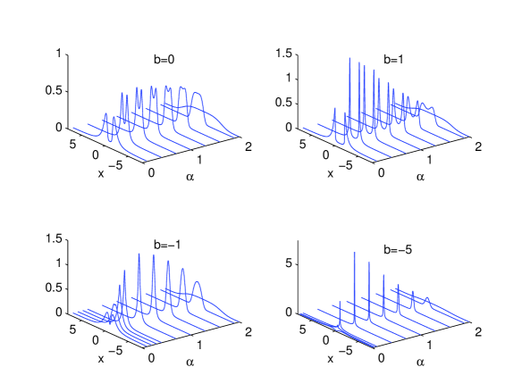
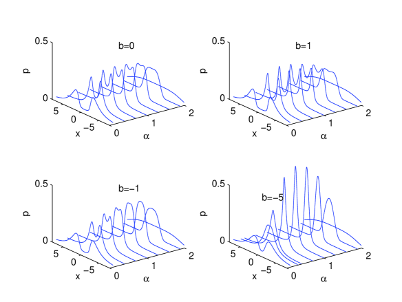
Figures 1 and 2 show the stationary probability density function $p(x)$ for $\epsilon=0.1$ and $\epsilon=0.9$, respectively. Here we only show several cases for $b=-5,-1,0,1$ and $\alpha=0.1,0.4,0.7,1.0,1.3,1.6,1.9,1.999$, as examples.

The probability density function $p(x)$ evolves from bimodal to unimodal, and then further changes to the flatter kurtosis shape for every fixed parameter $b$ in interval$(-10,0)$, as $\alpha$ value increases. The bifurcation occurs only for $b<0$, at some bifurcation value $\alpha*=\alpha(b,\epsilon)$, in our computational range. Note also that the $p(x)$ is bimodal for $b\geq 0$. This phenomenon is more evident when $\epsilon$ is larger in the range $(0,1)$; see Figure 2.

For fixed $b$ value, the probability density function $p(x)$ evolves from lower kurtosis to the higher one, and then changes to lower again, as $\alpha$ value increases.

Figure 1: Stationary probability density $p(x)$ for $\epsilon=0.1$

Figure 2: Stationary probability density $p(x)$ for $\epsilon=0.9$

3.3.2 Varying the parameter $b$

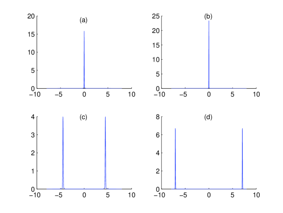
When $\alpha$ is approximately within in the interval $(0.4,1.6)$, the stationary density $p(x)$ becomes very spiky, and this is more evident when the magnitude of $b$ is large; see Figure 3.

Figure 3: Stationary probability density function $p(x)$ for $\epsilon=0.1$. (a) Corresponding to $\alpha=1$ and $b=-30$; (b) Corresponding to $\alpha=1$ and $b=-50$; (c) Corresponding to $\alpha=1.5$ and $b=20$; (d) Corresponding to $\alpha=1.5$ and $b=50$

3.3.3 Varying the parameter $\alpha$

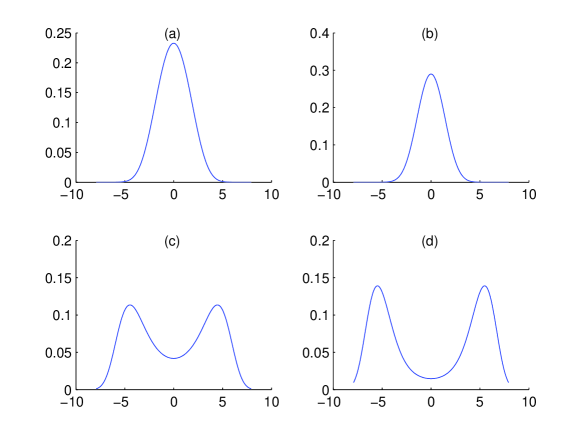
When $\alpha$ is approximately within in the interval $(1.9,2)$, the stationary density $p(x)$ becomes very flatter, and this is more evident when the value of $\alpha$ is close to 2; see Figure 4(subfigures (c) and (d) in both figures).

Figure 4: Stationary probability density function $p(x)$ for $\epsilon=0.1$ and $\alpha=1.999$. (a) Corresponding to $b=-30$; (b) Corresponding to $b=-50$; (c) Corresponding to $b=20$; (d) Corresponding to $b=30$

3.3.4 Impact of noise intensity $\epsilon$

Figure 5: Stationary probability density $p(x)$: $\alpha=0.3,\;b=-10$ for $\epsilon=0.1$, $\epsilon=0.9$ and $\epsilon=3$

Figure 6: Stationary probability density $p(x)$: $\alpha=0.7,\;b=-10$ for $\epsilon=0.1$, $\epsilon=0.9$ and $\epsilon=3$

Figure 7: Stationary probability density $p(x)$: $\alpha=1.6,\;b=5$ for $\epsilon=0.1$, $\epsilon=0.9$ and $\epsilon=3$

Figure 8: Stationary probability density $p(x)$: $\alpha=1.5,\;b=-8$ for $\epsilon=0.05$ and $\epsilon=0.1$

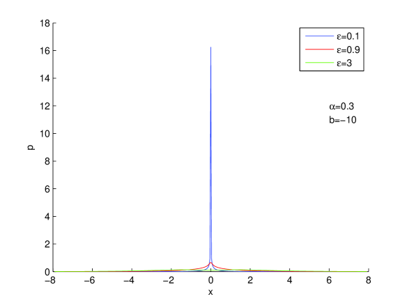
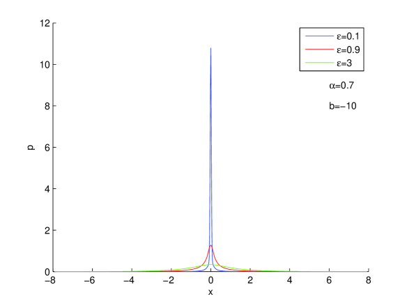
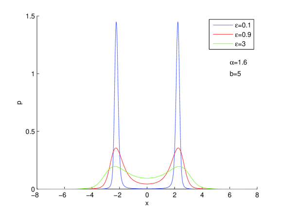
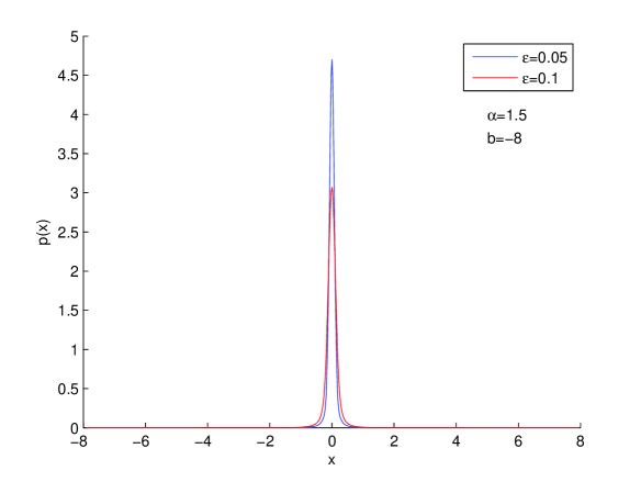
When the positive noise intensity $\epsilon$ is increased, we observe that the stationary density $p(x)$ becomes flatter (or less spiky) for fixed parameters $b$ and $\alpha$; see Figures 5-8. Thus the nonlocal integral term, due to Lévy jumps in the random forcing, in the steady Fokker-Planck equation (12) has a certain damping or diffusive effect.

3.3.5 A remark: Brownian motion vs. $\alpha-$stable Lévy motion

When $\alpha=2$, the corresponding Lévy motion is the Brownian motion. We take $\alpha$ close to $2$, the stationary density $p(x)$ are computed for various $b$ values; see Figures 3 and 4 (subfigures (c) and (d) in both figures), and also Figure 7. Here we also observe that $p(x)$ is bimodal for $b>0$, similar to the Brownian motion case in §3.2.

Acknowledgements. The authors would like to thank Xiaofan Li for helpful discussions about numerical schemes used in this research.

References

- [1] Albeverrio S, Rüdiger B, Wu J L. Invariant Measures and Symmetry Property of Lévy Type Operators. Potential Analysis, 2000,13: 147-168
- [2] Applebaum D. Lévy Processes and Stochastic Calculus. Cambridge University Press, Cambridge, UK, 2004.
- [3] Arnold L. Random Dynamical Systems. Springer-Verlag, New York, 1998.
- [4] Bertoin J. Lévy Processes, Cambridge University Press, Cambridge, U.K., 1998.
- [5] Chen H Q, Duan J Q, Li X F, etal. A computational analysis for mean exit time under non-Gaussian Lévy noises. Appl. Math. Comput. , 2011,218:1845-1856
- [6] H. Crauel and F. Flandoli, Additive noise destroys a pitchfork bifurcation. J. Dyn. Differ. Equ.,1998,10: 259-274
- [7] Ditlevsen P D. Observation of stable noise induced millennial climate changes from an ice record. Geophys. Res. Lett. ,1999,26: 1441-1444
- [8] Guckenheimer J, Holmes P. Nonlinear Oscillations, Dynamical Systems and Bifurcations of Vector Fields. Springer-Verlag, New York, 1983.
- [9] Janicki A, Weron A. Simulation and Chaotic Behavior of Stable Stochastic Processes, Marcel Dekker, Inc., 1994.
- [10] Kunita H. Stochastic differential equations based on Lévy processes and stochastic flows of diffeomorphisms. Real and stochastic analysis, 305–373, Trends Math., Birkhuser Boston, Boston, MA, 2004.
- [11] Navot I. An extension of the Euler-Maclaurin summation formula to functions with branch singularity. J. Math. and Phys.,1961,40: 271–276
- [12] Oksendal B. Applied Stochastic Control Of Jump Diffusions. Springer-Verlag, New York, 2005.
- [13] Otto S R, Denier J P. An Introduction to Programming and Numerical Methods in MATLAB. Springer-Verlag,london, 2005.
- [14] Peszat S, Zabczyk J. Stochastic Partial Differential Equations with Lévy Processes, Cambridge University Press, Cambridge, UK, 2007.
- [15] Sato K I. Lévy Processes and Infinitely Divisible Distributions, Cambridge University Press, Cambridge, 1999.
- [16] Schertzer D, Larcheveque M, Duan J , etal. Fractional Fokker–Planck equation for nonlinear stochastic differential equations driven by non-Gaussian Lévy stable noises. J. Math. Phys., 2001, 42: 200-212
- [17] Shlesinger M F, Zaslavsky G M, Frisch U.Lévy Flights and Related Topics in Physics (Lecture Notes in Physics, 450. Springer-Verlag, Berlin, 1995).
- [18] Woyczynski W A. Lévy processes in the physical sciences. In Lévy Processes: Theory and Applications, O. E. Barndorff-Nielsen, T. Mikosch and S. I. Resnick (Eds.), 241-266, Birkhäuser, Boston, 2001.