The Effects of Including Non-Thermal Particles in Flare
Loop Models

Abstract

In this work, we use HyLoop (Winter et al. 2011), a loop model that can incorporate the effects of both MHD and non-thermal particle populations, to simulate soft X-ray emissions in various situations. First of all, we test the effect of acceleration location on the emission in several XRT filters by simulating a series of post flare loops with different injection points for the non-thermal particle beams. We use an injection distribution peaked at the loop apex to represent a direct acceleration model, and an injection distribution peaked at the footpoints to represent the Alfvén wave interaction model. We find that footpoint injection leads to several early peaks in the apex-to-footpoint emission ratio. Second, we model a loop with cusp-shaped geometry based on the eruption model developed by Lin & Forbes (2000) and Reeves & Forbes (2005a), and find that early in the flare, emission in the loop footpoints is much brighter in the XRT filters if non-thermal particles are included in the calculation. Finally, we employ a multi-loop flare model to simulate thermal emission and compare with a previous model where a semi-circular geometry was used (Reeves et al. 2007). We compare the Geostationary Operational Environmental Satellite (GOES) emission from the two models and find that the cusp-shaped geometry leads to a smaller GOES class flare.

¹Harvard-Smithsonian Center for Astrophysics, USA

²Vanderbilt University, USA

1 Introduction

Hard X-ray observations show that a large fraction (50–75%) of the energy liberated in solar flares can go into the generation of non-thermal particles (e.g., Sui et al. 2005). Thus these particles are incredibly important for understanding the energy transfer in solar flares. However, many previous simulations of solar flares do not include the effects of the non-thermal particles directly (e.g., Hori et al. 1997, 1998; Reeves & Warren 2002; Warren 2006; Reeves et al. 2007). In this work, we use the HyLoop suite of codes to simulate flares with realistic geometries and we incorporate the effects of non-thermal particles in order to further the current understanding of energy transport in solar flares. This suite of codes has been described in detail previously in Winter et al. (2011).

2 HyLoop Model Description

The HyLoop suite of codes consist of two codes that work together to calculate the physical parameters in a loop due to MHD effects and particle acceleration. The MHD component of the codes is handled by the Solar Hydrodynamic Equation Codes (SHrEC), which solves the hydrodynamic equations along a loop in the following form:

$$\frac{\partial n_{\rm e}}{\partial t} = -\frac{1}{a}\frac{\partial}{\partial s}\left(an_{\rm e}V\right),$$ (1)

$$\frac{\partial V}{\partial t} = \frac{-1}{n_{\rm e}m_{\rm p}}\frac{\partial P}{\partial s}+g_{\parallel}-V\partial V,$$ (2)

$$\frac{\partial\epsilon}{\partial t} = -\frac{1}{a}\frac{\partial}{\partial s}\left(a\epsilon V\right)-\frac{P}{a}\frac{\partial}{\partial s}\left(aV\right)-E_{\rm Rad}$$ (3)

$$+\frac{1}{a}\frac{\partial}{\partial s}\left(aF_{\rm c}\right)+E_{\rm h}+E_{\rm NT},\$$

where $g_{\parallel}(s)$ is the component of acceleration due to gravity along the magnetic field, $P$ is the gas pressure, $a(s)$ is the non-uniform cross-sectional area of the loop, $\epsilon(s,t)$ is the internal energy density, $n_{\rm e}(s,t)$ is the electron density, $\mathbf{V}(s,t)$ is the bulk plasma velocity, $F_{\rm c}$ is the conductive flux, $E_{\rm Rad}$ is the radiative loss term, $E_{\rm h}$ is a background heating term, and $E_{\rm NT}(s,t)$, accounts for the energy gained by the thermal plasma via collisions with the non-thermal particle distribution.

The particles in HyLoop are handled by the Particle Tracking Codes (PaTC), which models the evolution of the non-thermal particles using direct Monte Carlo techniques. In PaTC the non-thermal distribution is treated as a series of test particles. These test particles are randomly drawn from probability distributions designed to represent the physics of a particular type of non-thermal beam. PaTC accounts for energy loss of the particles due to Coulomb collisions, and it also accounts for the effects of a non-uniform magnetic field. More details about the HyLoop suite of codes and their assumptions, boundary conditions, and initial conditions can be found in Winter et al. (2011).

3 Effects of Spatial Location of Heating Using HyLoop

It has long been assumed that non-thermal particles have been directly accelerated by the current sheet formed during the flare, with the particles being injected at the apex of post flare loops (Martens 1988; Hannah & Fletcher 2006). However, the number of non-thermal electrons implied by hard X-ray observations has often equaled or exceeded the total number of particles available in the acceleration region. In order to solve this “number problem”, theories have been proposed that have particle acceleration occurring in the denser chromosphere and transition region. Fletcher & Hudson (2008) have proposed a mechanism in which the energy of a flare accelerates non-thermal particles in the chromosphere via interactions with large-scale Alfvén waves.

Figure 1.: Injection distributions for the two different experiments: non-thermal particle injection peaked at the loop apex (left), and non-thermal particle injection at the loop footpoints (right).

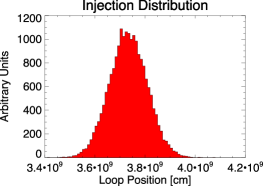
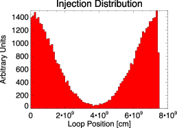
In order to construct a simple model that addresses this proposal, we use HyLoop to change the location of the non-thermal particle injection and examine the results on the soft X-ray emission. We simulate two particle acceleration scenarios: the acceleration of non-thermal particles at the loop apex (case a) and the acceleration of non-thermal particles by interactions with large-scale Alfvén waves, which occurs preferentially at the base of the loops (case b). We inject non-thermal particles into the loop using two different distributions, one steeply peaked at the loop apex, and one steeply peaked at the loop footpoints. The two distributions are shown in Figure 1.

An estimated flare energy of 10³⁰ erg is put into the production of non-thermal particles. These non-thermal particles are comprised entirely of electrons. The properties of the electrons are described by probability distribution functions. The pitch-angle probability distribution function is characterized by a single parameter, $\gamma$, which is set to $\gamma=0$ for both injection locations, corresponding to non-thermal particle acceleration via stochastic (turbulent) process at the loop apex (Winter et al. 2011). At the footpoints this pitch angle distribution also represents a stochastic process used to represent particle interactions with multiple wave-modes. The energy probability for each simulation is distributed as a single power-law function, $F(E)=E^{-\delta}$, with $\delta=3$.

A pre-flare loop is heated using a heating function $E_{\rm h}(s)=H\,T{{}^{\alpha}}P{{}^{\beta}}$ with $\alpha=3/2$ and $\beta=0$, which leads to heating primarily at the loop apex. The scaling constant, $H$, is chosen to give the loop a $T_{\rm max}=1.5$ MK. The loop geometry is defined by the Green (1965) current sheet model, and is the same geometry used in Winter et al. (2011).

Figure 2.: Simulated images for the XRT Ti-poly filter for (a) particle injection peaked at the apex, and (b) particle injection peaked at the footpoints. Cyan boxes indicate regions used to calculate ratios.

Figure 3.: Simulated apex-to-footpoint emission ratio for the Ti-poly (top), Be-thin (middle) and Be-med (bottom) filters. Results from the simulation with the particle injection peaked at the apex (case a) are shown in red and results from the simulation with particle injection peaked at the footpoints (case b) are shown in blue.

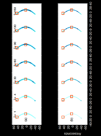
Soft X-ray emission is simulated in three XRT filters, the Ti-poly filter, the Be-thin filter and the Be-med filter. Images of the Ti-poly emission are shown in Fig. 2 for both the apex injection and the footpoint injection cases. In both cases, the footpoints show increased emission before the rest of the loop, and there are bright knots of emission along the loop. These bright knots are locations of density enhancements in the loop due to chromospheric evaporation. The bright knots appear at different locations at each time step in the two cases, indicating that that the timing of the chromospheric evaporation is different depending on the location of non-thermal particle injection.

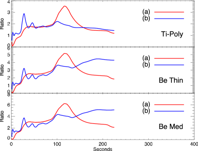
We calculate the ratio between the apex and footpoint emission for the Ti-poly, Be-thin, and Be-med filters for both particle injection profiles. The evolution of this ratio is shown in Figure 3. For the footpoint injection case, there is a clear and sharp peak in the ratio at about 30 s after the onset of the flare, followed by a secondary peak at about 45 s. There is also a broad peak in the ratio in all the filters at about 100 s, which is when the apex density peaks in this case, increasing the apex emission. In the apex injection case, there is a steady increase in the ratio starting at the flare onset, leading to a plateau between 40–80 s, and then a large peak at about 120 s. The large peak in the ratio occurs at the same time as the peak apex density in this case.

The ratio plots of Fig. 3 show that there are distinctly different signatures in the soft X-ray emission for particle injection at the apex versus at the footpoints. These results could be used to start looking for evidence of particle injection at the footpoints in order to confirm the theory put forth by Fletcher & Hudson (2008).

4 Cusped Flare Loop Geometry

Many flares have been observed to have a cusp-shaped geometry in the soft X-rays (e.g., Tsuneta et al. 1992; Forbes & Acton 1996; Reeves et al. 2008). This geometry is defined by the reconnecting magnetic fields that cause the release of energy in a solar flare. In the following section, we explore the effects of adding non-thermal particles to a loop with a cusp-shaped geometry that is defined by a model of reconnecting magnetic fields used to simulate coronal mass ejections and flares.

Figure 4.: (a) Magnetic configuration for the model prior to the loss of equilibrium. The current, $I$, is in the $z$ direction, out of the plane of the figure. (b) Magnetic configuration for the model after the eruption and formation of the current sheet. From Reeves (2006), reproduced by permission of the AAS.

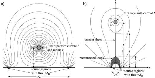
The model we use for the flare initiation is based on a version of the Lin & Forbes (2000) model that has been expanded to include gravity (Lin 2004; Reeves & Forbes 2005b). In this model, a flux rope is assumed to be in equilibrium prior to eruption due to a balance among the gravitational force, the magnetic tension force and the magnetic compression force. There are two surface sources that represent the sunspot magnetic field, and as these surface sources are quasi-statically brought closer together, a loss of equilibrium occurs and leads to an eruption. After the initiation of the eruption, a current sheet forms underneath the flux rope as shown in Figure 4. The current sheet is detached from the solar surface, allowing an arcade of reconnected magnetic loops to form between the localized sources as the eruption progresses.

The physical parameters in the model for the case we consider here are as follows:

$$\begin{array}[]{lll}M_{\rm A}=0.01,&&h_{0}=5\times 10^{9}\>\mbox{cm},\\ m=2.1\times 10^{16}\>\mbox{g},&&\rho=1.67\times 10^{-16}\>\mbox{g cm${}^{-3}$},\\ \ell=10^{10}\>\mbox{cm},&&B_{0}=25\>\mbox{G},\end{array}$$

where $m$ is the mass of the flux rope, $\rho$ is the atmospheric density at the base of the corona, $B_{0}$ is the background magnetic field strength, $\ell$ is the length of the flux rope, and $h_{0}$ is the height of the flux rope at the maximum current point on the equilibrium curve—a convenient point to use for normalization purposes (see Lin & Forbes 2000). $M_{\rm A}$ is the inflow Alfvén Mach number, which specifies the reconnection rate, and it is fixed at the midpoint of the current sheet. The parameters listed above are chosen because they are the same as those used in modeling one of the flares studied in Reeves (2006) and Reeves & Moats (2010).

Figure 5.: The geometry of the flare loops in this model, as defined by the reconnecting magnetic fields. The boundaries of the loops are contours of the vector potential $A$ taken 20 s apart. The cross sectional area, $a(s)$, is defined by the width between the loop boundaries. A chromosphere is assumed to be at a height $\ell$ above the bottom of the loop, to prevent the cross-sectional area from going to zero.

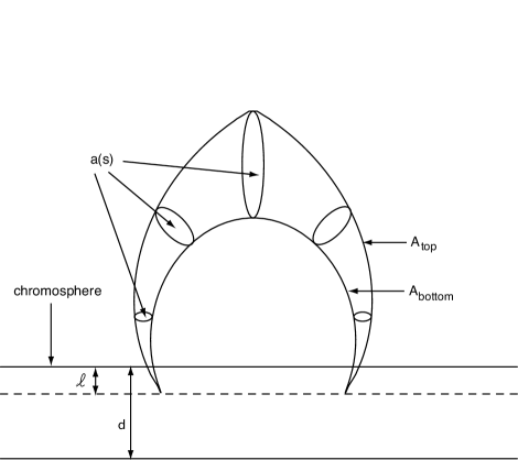
We take as the boundaries of our loop contours of the vector potential $A$ that travel through the reconnection region and form loops in the Lin & Forbes (2000) reconnection model. The top and bottom boundaries are contours of the vector potential that travel through the reconnection region 20 s apart. This geometry is shown in Figure 5. The current version of the HyLoop code cannot take into account the shrinkage of the loop, so we define the loop geometry using a time late in the flare evolution, after the shrinkage ceases to be important. We then take the coordinates of the loop and use them to define the loop geometry in HyLoop.

We assume that the cross section of the loop, $a(s)$, is a circular cross section with the diameter equal to the width between the upper and lower boundaries of the loop. Because there are singularities in the magnetic field at the footpoints of the loop, the cross-sectional area would go to zero there (see Figure 5). So, we assume that the chromosphere is a height $\ell=10^{7}$ cm above the bottom of the loop, in order to avoid the singularities there. We also assume for a boundary condition that the chromosphere is held at a temperature of $10^{4}$ K, and that it extends to a depth of $d=2\times 10^{8}$ cm. This boundary condition is slightly different from the one used in Winter et al. (2011), but is commensurate with boundary conditions used in other flare modeling codes (e.g., Mariska 1987).

For this experiment, we input energy in two ways. For the first case, we input energy that is completely thermal in nature. For the second case, we input 100% of the energy as non-thermal particles. For both cases, the total energy input into the loop is $1.35\times 10^{29}$ erg, and it is input at the apex of the loop. For the non-thermal case, the energy is distributed as a single power-law function, $F(E)=E^{-\delta}$, with $\delta=3$, as in the experiment described in Section 2. The pitch angle of the non-thermal particles is distributed around zero, so that the velocities of the particles are primarily aligned along the magnetic field.

Figure 6.: Temperature (left) and density (right) for several different times during the beginning of the flare for a case with no non-thermal particles (black) and a case where all of the energy is put into non-thermal particles (red). Time is in seconds.

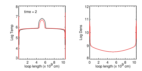
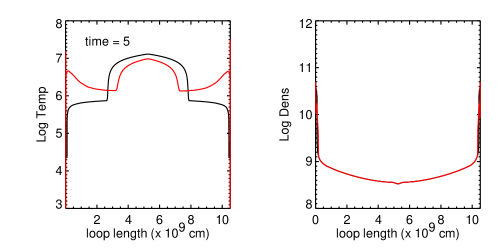
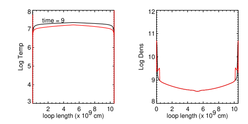
Figure 6 shows the evolution of the temperature and emission measure during the first few seconds of the flare. For the non-thermal case, plotted in red, the figure clearly shows that the footpoints heat up more quickly than in the thermal case. This heating happens because the non-thermal particles stream down the magnetic field lines within the first few seconds after initiation and deposit their energy in the chromosphere, causing heating at the base of the loop.

Figure 7.: XRT Ti-poly emission along the loop for several different times during the beginning of the flare for a case with no non-thermal particles (black) and a case where all of the energy is put into non-thermal particles (red).

Figure 8.: XRT Ti-poly emission for a multi-stranded flare using the HyLoop code.

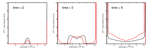
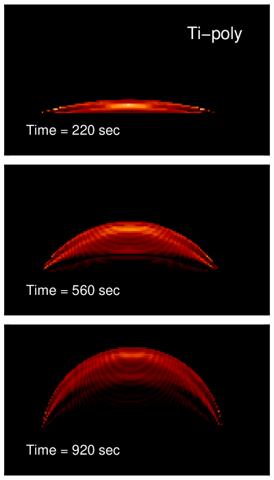
Figure 7 shows the XRT Ti-poly emission as a function of loop length for the thermal and non-thermal energy distributions for several times early in the flare evolution. Both cases show a peak in the loop-top emission early in the flare. However, because of the elevated temperatures in the footpoints in the loop with the purely non-thermal energy input, there is more footpoint emission in that loop by 5 s than in the loop with only thermal energy input.

5 Multi-Stranded Flare

The results presented above are interesting, but they are only calculated for a single loop. However, there is growing consensus in the solar community that flares consist of many loops (Hori et al. 1998; Reeves & Warren 2002; Warren & Doschek 2005; Reeves et al. 2007). Ultimately, we will use HyLoop to simulate a multi-stranded flare that includes the effects of non-thermal particles. Here, we use HyLoop to simulate a multi-stranded flare with completely thermal energy input, an experiment that takes less in the way of computing resources than the full non-thermal case. The geometry in these loops is defined as in the previous section, with a cusp-shaped top and tapered ends.

Using the same methodology as in Reeves et al. (2007), we simulate 140 discrete loops to make up the flare arcade, with a new loop appearing every 20 s. The loss-of-equilibrium model parameters are the same as in the previous section. The input heating rate in each loop is given by

$$\epsilon(s,t)=\epsilon_{0}+f(s)\,g(t)\,\epsilon_{\rm flare},$$ (4)

where $\epsilon_{0}$ is the background heating parameter, $g(t)$ is a triangular function, and $f(s)$ is a Gaussian function given by $\exp[-(s-s_{0})^{2}/2\sigma^{2}]$, where $s_{0}$ is the apex of the loop, $\sigma$ is the width of the heating region (taken to be $10^{8}$ cm), and $\epsilon_{\rm flare}$ is the constant amplitude of the heating. The total energy input into each loop is calculated from the Poynting flux into the current sheet in the loss-of-equilibrium calculation, as in Reeves et al. (2007).

Figure 9.: GOES 1–8 Å light curves for flares simulated using HyLoop with a cusp-shaped geometry (right) and SOLFTM with a semicircular geometry (left).

Using this energy input, we simulate a multi-stranded flare and the XRT Ti-poly intensity. Figure 8 shows the evolution of the simulated Ti-poly emission for the multi-stranded flare. The effects of the geometry can be clearly seen in this figure, since the ends of the loops are very tapered as compared to the tops of the loops. In the first two frames, a compact brightening can be seen at the top of the flare arcade. This brightening is caused by density fronts colliding at the tops of the loops to create enhanced emission measure there. This effect was found previously with semi-circular loops by Reeves et al. (2007). This loop-top source persists because new loops are constantly forming and producing these colliding density fronts as the reconnection progresses. Late in the flare, at $t=920$ s, there is still a small enhancement in the emission at the flare loop top, but is is not as strong as early in the flare, since the loops that are reconnected late in the flare have a lower volumetric heating rate than those energized early in the flare.

In order to understand the effects the cusp-shaped geometry has on the simulated flare, we compare two different models: HyLoop, with the cusp-shaped geometry described in the previous section, and the NRL Solar Flux Tube Model (SOLFTM; see Mariska 1987) with semi-circular loops. We model the GOES flux in each simulated flare, as shown in Figure 9. We find that the HyLoop model with the cusp-shaped geometry results in much weaker flare X-ray emission than the SOLFTM model with the semi-circular geometry. The cusp-shaped geometry results in the weaker flare because there is a smaller area in the loop footpoint for the heat to be deposited, resulting in smaller evaporation flows and less chromospheric evaporation in the cusp-shaped loop.

6 Conclusions

We have performed several different experiments using the HyLoop code and found that non-thermal particles can have a profound effect on the soft X-ray signal from a flare. We have shown that the existence of non-thermal particles in a beamed distribution will cause the footpoints of the flare to heat up faster than if no non-thermal particles are present. The location of the input of the non-thermal particles will have an effect on the evolution of the apex-to-footpoint ratio, with non-thermal particles input at the footpoints causing many small peaks in the ratio that are not seen if the particles are input in the loop-top. This information may be used in conjunction with observational signatures to confirm or deny the injection of non-thermal particles at the footpoints.

We have also investigated the effects of simulating a flare with a cusp-shaped geometry taken from the magnetic reconnection model of Lin & Forbes (2000). We find that emission in the loop footpoints is much brighter in the XRT filters if non-thermal particles are included in the calculation because the beamed particles quickly travel to the chromosphere and deposit their energy there. We also find that the cusp shape of the loops causes a bottleneck in the loop that causes a smaller upflow of density than if a semi-circular loop is used. The smaller upflow leads to lower densities in the loop, and thus a lower GOES class for the flare.

In the future, we plan to model multi-threaded flare arcades using HyLoop to incorporate the effects of non-thermal particles in each of the individual strands.

Acknowledgments

Hinode is a Japanese mission developed and launched by ISAS/JAXA, with NAOJ as domestic partner and NASA and STFC (UK) as international partners. It is operated by these agencies in cooperation with ESA and NSC (Norway). KKR and HDW are supported by contract NNM07AB07C from NASA to SAO. Additional support for KKR comes from the NSF-SHINE program, grant number ATM-0752257. Additional support for HDW comes from NASA grant NNX09AB18G-R. The work of NLL was supported by the NSF-REU solar physics program at CfA, grant number ATM-0851866.

References

- Fletcher & Hudson (2008) Fletcher, L., & Hudson, H. S. 2008, ApJ, 675, 1645
- Forbes & Acton (1996) Forbes, T. G., & Acton, L. W. 1996, ApJ, 459, 330
- Hannah & Fletcher (2006) Hannah, I. G., & Fletcher, L. 2006, Solar Phys., 236, 59
- Hori et al. (1997) Hori, K., Yokoyama, T., Kosugi, T., & Shibata, K. 1997, ApJ, 489, 426
- Hori et al. (1998) — 1998, ApJ, 500, 492
- Lin (2004) Lin, J. 2004, Solar Phys., 219, 169
- Lin & Forbes (2000) Lin, J., & Forbes, T. G. 2000, J. Geophys. Res., 105, 2375
- Mariska (1987) Mariska, J. T. 1987, ApJ, 319, 465
- Martens (1988) Martens, P. C. H. 1988, ApJ, 330, L131
- Reeves (2006) Reeves, K. K. 2006, ApJ, 644, 592
- Reeves & Forbes (2005a) Reeves, K. K., & Forbes, T. G. 2005a, ApJ, 630, 1133
- Reeves & Forbes (2005b) — 2005b, in Coronal and Stellar Mass Ejections, IAU Symposium 226, edited by K. Dere, J. Wang, & Y. Yan (Cambridge: Cambridge University Press), 250
- Reeves & Moats (2010) Reeves, K. K., & Moats, S. J. 2010, ApJ, 712, 429
- Reeves et al. (2008) Reeves, K. K., Seaton, D. B., & Forbes, T. G. 2008, ApJ, 675, 868
- Reeves & Warren (2002) Reeves, K. K., & Warren, H. P. 2002, ApJ, 578, 590
- Reeves et al. (2007) Reeves, K. K., Warren, H. P., & Forbes, T. G. 2007, ApJ, 668, 1210
- Sui et al. (2005) Sui, L., Holman, G. D., & Dennis, B. R. 2005, ApJ, 626, 1102
- Tsuneta et al. (1992) Tsuneta, S., Hara, H., Shimizu, T., Acton, L. W., Strong, K. T., Hudson, H. S., & Ogawara, Y. 1992, PASJ, 44, L63
- Warren (2006) Warren, H. P. 2006, ApJ, 637, 522
- Warren & Doschek (2005) Warren, H. P., & Doschek, G. A. 2005, ApJ, 618, L157
- Winter et al. (2011) Winter, H. D., Martens, P., & Reeves, K. K. 2011, ApJ, 735, 103