Numerical method for non-linear steady-state transport in one-dimensional correlated conductors

Abstract

We present a method for investigating the steady-state transport properties of one-dimensional correlated quantum systems. Using a procedure based on our analysis of finite-size effects in a related classical model ($LC$ line) we show that stationary currents can be obtained from transient currents in finite systems driven out of equilibrium. The non-equilibrium dynamics of correlated quantum systems is calculated using the time-evolving block decimation method. To demonstrate our method we determine the full $I$–$V$ characteristic of the spinless fermion model with nearest-neighbour hopping $t_{\text{H}}$ and interaction $V_{\text{H}}$ using two different setups to generate currents (turning on/off a potential bias). Our numerical results agree with exact results for non-interacting fermions ($V_{\text{H}}=0$). For interacting fermions we find that in the linear regime $eV\ll 4t_{\text{H}}$ the current $I$ is independent from the setup and our numerical data agree with the predictions of the Luttinger liquid theory combined with the Bethe Ansatz solution. For larger potentials $V$ the steady-state current depends on the current-generating setup and as $V$ increases we find a negative differential conductance with one setup while the currents saturate at finite values in the other one. Both effects are due to finite renormalized bandwidths.

I Introduction

Much of our understanding of electronic transport in solids is based on a picture of weakly-interacting charge carriers such as Fermi liquid quasi-particles. One-dimensional electron systems are well-known examples where this approximation fails. The low-energy physics of these systems is described by the Tomonaga-Luttinger liquid (TLL) theory and is realized in quantum wires such as carbon nanotubes, nanowires in semiconductor heterostructures, or metal atomic chains on surface substrates.Schoenhammer02 ; Giamarchi03 ; Schoenhammer04

The transport properties of one-dimensional correlated systems have been extensively studied during the last two decades.Giamarchi03 ; Schoenhammer04 ; Yacoby04 ; Zotos04 ; Kawabata07 A major goal is to determine and understand the current-voltage characteristic $I-V$ of various systems made of quantum dots and wires. Most of these studies have been restricted to a regime where the energy scale of the current-generating electromagnetic field or potential bias is small in comparison to the energy scale of the unperturbated systems (i.e., the band width in lattice models and the Fermi velocity in continuum models). The non-linear regime has mostly been investigated in quantum contact problems, where the interaction is confined to a small region of the system. For instance, non-linear current-voltage characteristics have been calculated within the TLL theory such as the power-law $I\sim V^{\alpha}$ behaviour for the transport through a weak link Kane92 ; Furusaki93 or the exact $I(V)$ curve for the current through a point contact in a fractional quantum Hall edge state device.Fendley95 ; Komnik11 However, the TLL theory is limited to low-energy excitations with linear dispersion and thus to potential biases $V$ which are weak compared to the band width. Only recently the implications of a non-linear dispersion have started to be considered.Barak10 Thus current-voltage characteristics from the TLL theory are actually limited to a weak-bias regime.

There are few works presenting full current-voltage characteristics with a voltage up to the largest energy scale of the system (for instance, see Refs. Boulat08, ,  Heidrich09a, , and Carr11, ) and none is concerned with one-dimensional correlated conductors. Thus transport properties beyond linear response are poorly understood. We believe that it is important to attain a better knowledge of the non-linear transport properties in one-dimensional correlated conductors. First, the validity of weak-bias approaches can be confirmed only if one obtains some quantitative estimates of non-linear effects. Moreover, non-linear devices play a significant role in electronics and studies of non-linear dynamics are required to reveal the full potential functionality of quantum wires as electronic circuit components.

In this work we develop and apply a method for investigating the zero-temperature DC transport properties of one-dimensional correlated conductors for potential biases up to the order of the band width. For this purpose we study a well-known one-dimensional lattice model described by the half-filled spinless fermion Hamiltonian with nearest-neighbour repulsion. Even though this model is exactly solvable by the Bethe Ansatz and the low-energy physics are determined by the generic TLL phenomenologyGiamarchi03 ; Schoenhammer04 , its transport properties in the non-linear regime cannot be obtained analytically.

To determine the transport properties we simulate the quantum dynamics of single chains which are driven out of equilibrium by a potential bias between the left- and right-hand halves of the chain and calculate the resulting currents through the middle bond. The simulation of out-of-equilibrium quantum many-particle systems is one of the major challenges in computational physics. Recently, a family of numerical methods has been developed to simulate the real-time evolution of quantum lattice systems such as one-dimensional Hamiltonians with short-range interactions.Schollwoeck06 ; Noack08 ; Schollwoeck11 The most prominent ones are the time-dependent Density-Matrix Renormalization Group (td-DMRG) and the time-evolving block decimation (TEBD) method.Vidal03 ; Vidal04 Various flavours of td-DMRG have been successfully applied in studies of quantum many-body dynamics. In particular, they have proven to be promising tools for investigating electronic transport in strongly correlated nanostructures and one-dimensional conductors.Boulat08 ; Heidrich09a ; Cazalilla02 ; Luo03 ; Cazalilla03 ; Schmitteckert04 ; Al-Hassanieh06 ; Kirino08 ; Heidrich09b ; Kirino10 ; Heidrich10 ; Znidaric11 ; Jesenko11

Surprisingly, the original TEBD methodVidal03 ; Vidal04 has not been applied to electronic transport problems yet. Both td-DMRG and TEBD methods can be described within a common mathematical framework, the matrix product quantum states.Schollwoeck11 ; Daley04 ; Jeckelmann08 Their accuracy and efficiency depend essentially on the amount of entanglement in the quantum system and should be similar. Admittedly, the TEBD algorithm is restricted to a small family of systems (one-dimensional Hamiltonians or ladder systems with nearest-neighbour interactions only) while td-DMRG techniques are more versatile. However, the TEBD algorithm is naturally parallelizable and thus fully scalable, which is a required feature in high-performance computing, while the efficient parallelization of the DMRG algorithms remains an open challenge.Hager04 ; Schmitteckert07 In this work we employ the TEBD method for computing the non-equilibrium dynamics of the spinless fermion model.

With the TEBD method we can compute the non equilibrium quantum dynamics of lattice models with a finite number of sites $N$ over a finite period of time $t$. As we are primarily interested in determining the DC transport properties, TEBD results must be extrapolated to the thermodynamic limit $N\rightarrow\infty$ and to the steady-state limit $t\rightarrow\infty$. However, finite-size and finite-time effects are very complex in these out-of-equilibrium quantum systems (for instance, see Ref. Branschaedel10, ) and extrapolations are difficult because we know very little about the scaling of currents with system size $N$ and time $t$. For this reason we have investigated this scaling in an exactly solvable classical model, the so-called $LC$ line. Using this information we have developed a method for quantum systems which allows us to obtain reliable quantitative results for stationary currents $I$ from numerical data for rather small system sizes and short simulation times.

In this paper we show that our extrapolation approach allows one to determine the full $I-V$ curves of interacting one-dimensional conductors using the spinless fermion model for illustration. In the non-interacting case this model can be solved exactly using the equation of motion method. The outcomes of this special case confirm our extrapolation method and reveal a negligible numerical error for the TEBD simulation results. For interacting fermions comparisons with predictions from the TLL theory and the Bethe-Ansatz solution confirm the validity of our method in the linear response regime. While for the linear regime the specific setup does not matter, it is highly decisive for the non-linear current-voltage characteristics. We basically distinguish between two different ways of creating a current flow.Branschaedel10 In the first setup (I) we apply an initial voltage and calculate the ground state which has different particle numbers in its two halves and then let the system evolve with an overall equal on-site potential. In the second setup (II) we calculate the ground state without a potential difference but turn it on for the real time evolution. We have found that while the general shape of the current-curve as a function of time is dominated by classical effects (i.e., which are also found in the $LC$ line model), the current-voltage characteristics are primarily determined by the chosen setup. For setup (I) the system shows a positive differential conductance for the full voltage-range and saturates at a finite value for very large potential differences. For the second setup (II) the linear response coincides with the one for setup (I) but for higher voltages we observe a negative differential conductance. Both effects are also present in the non-interacting case and come from the finite bandwidth and the non-linear dispersion (i.e., the energy-dependent density of states) of the excitations.Branschaedel10 ; Baldea10

Our paper is organized as follows: In the next section we introduce the spinless fermion model, and the methods used in this work. In the third section we investigate the classical $LC$ line to explain the basic behaviour of the current in finite and infinite one-dimensional chains and derive our method to extrapolate the stationary current from finite system results. In the fourth section we describe finite-size effects and the convergence to a stationary current for infinite system sizes, while the $I-V$ characteristic of the spinless fermion model and comparisons with exact results are shown in the fifth section. Finally, we summarize our findings in the last section. Some calculations are detailed in appendices.

II Model and methods

II.1 Spinless fermion model

We consider a one-dimensional lattice model representing correlated conductors driven out of equilibrium by a potential bias. For spinless fermions the Hamiltonian without a potential bias is

$$H_{0}= -t_{\text{H}}\sum_{j=1}^{N-1}(c_{j}^{\dagger}c_{j+1}+c_{j+1}^{\dagger}c_{j})$$ (1)

$$+V_{\text{H}}\sum_{j=1}^{N-1}\left(n_{j}-\frac{1}{2}\right)\left(n_{j+1}-\frac{1}{2}\right)$$

where $t_{\text{H}}$ denotes the hopping amplitude between nearest-neighbour sites, $V_{\text{H}}$ is the Coulomb repulsion between spinless fermions on nearest-neighbour sites, and $n_{j}=c_{j}^{\dagger}c_{j}$. At half filling ($N/2$ fermions in the $N$-site lattice) this Hamiltonian describes an ideal conductor for $-2t_{\text{H}}<V_{\text{H}}\leq 2t_{\text{H}}$. It can be interpreted as a system of spin-polarized electrons.

The low-energy behaviour of this lattice model is described by the TLL theory.Giamarchi03 ; Schoenhammer04 The generic properties of a TLL are determined by two parameters: The velocity of elementary excitations (renormalized Fermi velocity) $v$ and a dimensionless parameter $K$. From the Bethe Ansatz solution we know the relation between TLL parameters and the parameters $t_{\text{H}}$ and $V_{\text{H}}$ of the spinless fermion model at half filling

$$v=\pi\frac{a_{L}t_{\text{H}}}{\hbar}\sqrt{1-\left(\frac{V_{\text{H}}}{2t_{\text{H}}}\right)^{2}}\left[\arccos\left(\frac{V_{\text{H}}}{2t_{\text{H}}}\right)\right]^{-1}$$ (2)

and

$$K=\frac{\pi}{2}\left[\pi-{\arccos}\left(\frac{V_{\text{H}}}{2t_{\text{H}}}\right)\right]^{-1}$$ (3)

where $a_{L}$ is the lattice constant. To drive the system out of equilibrium we a use step-like potential bias between the left- and right-hand halves of the chain

$$H_{B}=\frac{\Delta\epsilon}{2}\left(\sum_{j=1}^{N/2}n_{j}-\sum_{j=N/2+1}^{N}n_{j}\right).$$ (4)

The potential energy step is set by $\Delta\epsilon=|eV|$ where $V$ is the voltage bias and $e$ is the elementary charge. It is possible to use a smoother potential profile but the results for the stationary current using our extrapolation method are only slightly affected by the specific shape as long as the non-constant part in the middle is rather smooth and locally confined.

Figure 1: One-dimensional conductor consisting of two coupled leads. A bias between its right- and left-hand halves is applied and the current is measured in the middle of the system at the junction between both sides (dashed connection).

The above system can be seen as two coupled interacting leads made of the sites $\{1\dots\frac{N}{2}\}$ and $\{\frac{N}{2}+1\dots N\}$, respectively, see Fig. 1. The coupling is given by a hopping term $t^{\prime}_{H}$ between the left- and right-hand sides of the system (i.e., between site $N/2$ and site $N/2+1$) and an additional coupling $V^{\prime}_{\text{H}}(\ n_{N/2}-1/2)(\ n_{N/2+1}-1/2)$. Here we discuss the homogeneous system only ($t^{\prime}_{H}=t_{\text{H}}$ and $V^{\prime}_{\text{H}}=V_{\text{H}}$) but our approach can be easily extended to systems with a weak link $t^{\prime}_{H}<t_{\text{H}}$ representing the tunneling through a nanostructureCazalilla02 or with a site representing a quantum dot, such as the Interacting Resonant Level Model (IRLM)Boulat08 , as well as to systems with a few additional sites intercalated between both leads and representing nanostructures with internal degrees of freedom.Schmitteckert04

The current operator between the pair of sites $(k,k+1)$ is

$$j_{k}=i\frac{et_{\text{H}}}{\hbar}\left(c_{k}^{\dagger}c_{k+1}-c_{k+1}^{\dagger}c_{k}\right).$$ (5)

For a given (time-dependent) quantum state we define the current flowing between both halves of the system (see Fig. 1) as the expectation value of the current operator for the site pair in the middle of the system

$$J(t)=\left\langle j_{N/2}\right\rangle.$$ (6)

We note that

$$J(t)=-\frac{d}{dt}Q_{L}(t)=\frac{d}{dt}Q_{R}(t)$$ (7)

where

$$Q_{L}(t)=-e\sum_{k=1}^{N/2}\langle n_{k}\rangle\quad\text{and}\quad Q_{R}(t)=-e\sum_{k=N/2+1}^{N}\langle n_{k}\rangle$$ (8)

are the (time-dependent) charges in the left- and right-hand halves of the chain, respectively. As the number of particles $n$ is conserved in our models, $Q_{L}(t)+Q_{R}(t)=-e\cdot n=\text{const}$. The stationary current is a constantly flowing current in an infinitely large system after the settling time

$$\bar{J}=\lim_{t\rightarrow\infty}\lim_{N\rightarrow\infty}J(t)$$ (9)

and according to the TLL theory in the linear regime (small $\Delta\epsilon$) it is given byGiamarchi03

$$\bar{J}=\frac{e^{2}}{h}KV=\frac{e}{h}K\Delta\epsilon\quad\text{for}\quad V\geq 0.$$ (10)

We set $t_{\text{H}}=a_{L}=1$ for all numerical simulations and, if units are not given explicitly, $e=\hbar=1$.

In this work both setups used to generate a current (see the next section) lead to an overall half-filled system. Thus in the weak potential bias regime both system halves remain approximately half-filled at all times. Consequently, we expect that the current is given by the Luttinger liquid prediction (10) together with the Bethe Ansatz result (3) in the linear response regime.

II.2 Setups for non-equilibrium simulations

We employ two different setups to generate currents in the lattice models. Branschaedel10

Figure 2: Setup (I): The charge reservoirs (two halves: source and drain) have different potentials but are coupled for $t=0$ while for $t>0$ the potential difference is set to $\Delta\epsilon=0$ instantaneously.

In the first one (I) we prepare the system at time $t=0$ in the ground state $|\phi(\Delta\epsilon\neq 0)\rangle$ of the Hamiltonian $H=H_{0}+H_{B}$ (i.e. with potential bias), see Fig. 2. For later times $t>0$ we let the system evolve according to the Hamiltonian $H_{0}$ (i.e. without potential bias)

$$|\psi(t>0)\rangle=\exp\left(-i\frac{H_{0}t}{\hbar}\right)|\phi(\Delta\epsilon\neq 0)\rangle.$$ (11)

This setup describes an inhomogeneous initial state with more particles in one half of the system than in the other one. Thus particles flow from one side to the other one for $t>0$. It corresponds to a one-dimensional scattering experiment in which particles are emitted on one side of the system with energies between $[-\Delta\epsilon/2,\Delta\epsilon/2]$, scattered at the junction between both system halves, and then (partially) transmitted to the opposite side. This picture of transport through junctions is often used in theoretical investigations.

Figure 3: Setup (II): The charge reservoirs (two halves: source and drain) are in equilibrium and coupled with $t_{\text{H}}$ and $V_{\text{H}}$ for $t=0$. For $t>0$ a potential difference $\Delta\epsilon>0$ is applied.

In the second setup (II) we prepare the system at time $t=0$ in the ground state $|\phi(\Delta\epsilon=0)\rangle$ of the Hamiltonian $H_{0}$ (i.e., without potential bias). For later times $t>0$ the time evolution of the system is determined by the Hamiltonian $H=H_{0}-H_{B}$, i.e. with a potential bias that causes the current to flow in the same direction as in setup (I)

$$|\psi(t>0)\rangle=\exp\left(-i\frac{(H_{0}-H_{B})t}{\hbar}\right)|\phi(\Delta\epsilon=0)\rangle.$$ (12)

Setup (II) describes the evolution of an initially homogeneous state under the influence of a potential gradient, see Fig. 3. Thus it corresponds more closely to the actual experimental situation with a voltage source generating a current in a conducting wire.

We should point out that in setup (I) the two leads are decoupled with respect to the Coulomb-interaction $V^{\prime}_{\text{H}}$ for the calculation of the ground state. Our tests have revealed that otherwise a strong dependency of the stationary current on the system size appears, that is, for smaller system sizes the stationary current becomes higher but for $N\rightarrow\infty$ it approaches the same constant value as the value one gets with $V^{\prime}_{\text{H}}=0$ for $t=0$. Choosing $V^{\prime}_{\text{H}}=0$ for the computation of the ground state therefore decreases the finite-size error.

Generally, currents (6) calculated with the states (11) and (12) are different. In the strong-bias limit $|\Delta\epsilon|\gg t_{\text{H}},V_{\text{H}}$ it is easy to show that the steady-state current remains finite for the first setup while it vanishes for the second one. Recently, it has been reported that initial conditions (quenching an interaction term or a tunneling term) can also alter the steady-state current flowing through a quantum point contact between two TLL leads which have been driven out of equilibrium by an external bias.Perfetto10 In the weak-bias limit $|\Delta\epsilon|\ll t_{\text{H}}$, however, a simple perturbation calculation shows that both setups yield the same linear response for the stationary current. Thus in this regime both setups can be used indifferently but in the non-linear regime we must distinguish them.

In most theoretical studies the potential bias switching is not instantaneous but adiabatic. This can also be used in numerical simulations, for instance, see Refs. Cazalilla02, and Kirino10, . Our tests do not reveal any significant differences for the steady-state current depending on the switching rate as long as the potential changes in a time scale which is much smaller than the time scale associated with the motion of particles from one reservoir to the other one. Since our extrapolation method is designed to work with an instantaneous change in the potential difference and as numerical simulations are simpler with it, we prefer this approach.

II.3 One-particle equation of motion

Without Coulomb-interaction $V_{\text{H}}(=V^{\prime}_{\text{H}})=0$ the spinless fermion model, described by the Hamiltonian (1), reduces to the tight-binding model (non-interacting fermions without spin degree of freedom). A one-dimensional chain in the tight-binding model can be described by the single particle reduced density matrix

$$\mathcal{G}_{ij}(t):=\langle{\Psi(t)}|c_{i}^{\dagger}c_{j}|{\Psi(t)}\rangle$$ (13)

where the time evolution is given by the one-particle equation of motion

$$\frac{d}{dt}\mathcal{G}(t)=\frac{i}{\hbar}[H_{t>0}^{(1)},\mathcal{G}(t)].$$ (14)

$H_{t>0}^{(1)}$ denotes the single particle Hamilton matrix of size $N\times N$ with which the system is evolved in time. More precisely $H_{t>0}^{(1)}$ is the one-particle representation of $H_{0}$ or $H_{0}+H_{B}$ depending on the specific setup. The particle number expectation values coincide with the diagonal terms of the reduced density matrix

$$\langle{n_{k}(t)}\rangle=\langle{\Psi(t)}|c_{k}^{\dagger}c_{k}|{\Psi(t)}\rangle=\mathcal{G}_{kk}(t)$$ (15)

and the expectation value for the current operator (5) from site $k$ to $k+1$ can be taken from off-diagonal entries

$$\langle{j_{k}(t)}\rangle=i\frac{et_{\text{H}}}{\hbar}[\mathcal{G}_{k,k+1}(t)-\mathcal{G}_{k+1,k}(t)].$$ (16)

Consequently, the dynamics of a tight-binding chain can be computed numerically without additional truncation error with a runtime of $\mathcal{O}(N^{3})$ for any point in time.

II.4 TEBD method

The TEBD methodVidal03 ; Vidal04 is based on a specific representation of quantum states by matrix product states (MPS). For an $N$-site lattice it is generally written

$$|\Psi\rangle= \sum_{\{j_{k}\}}\Gamma^{[1]j_{1}}\lambda^{[1]}\Gamma^{[2]j_{2}}\lambda^{[2]}\dots$$ (17)

$$\dots\Gamma^{[N-1]j_{N-1}}\lambda^{[N-1]}\Gamma^{[N]j_{N}}|j_{1}j_{2}\dots j_{N}\rangle$$

where $|j_{1}j_{2}\dots j_{N}\rangle$ designs the states of the occupation number basis, $\lambda^{[k]}(k=1,2,\dots,N-1)$ are positive definite diagonal matrices and $\Gamma^{[k]j_{k}}(k=1,2,\dots,N)$ are matrices satisfying orthogonality conditions

$$\sum_{j_{k}}\left(\Gamma^{[k]j_{k}}\right)^{\dagger}\left(\lambda^{[k-1]}\right)^{2}\Gamma^{[k]j_{k}} = I,$$

$$\sum_{j_{k}}\Gamma^{[k]j_{k}}\left(\lambda^{[k]}\right)^{2}\left(\Gamma^{[k]j_{k}}\right)^{\dagger} = I.$$ (18)

Sums over an index $j_{k}$ run over a complete basis of the site $k$ (for instance 2 states for the spinless fermion model). Every quantum state of the Fock space associated with a finite lattice can be represented exactly in this form if the matrix dimensions can be as large as the square root of the Fock space dimension (for instance $2^{N/2}$ for the spinless fermion model). In numerical computations, however, the matrix dimension must be kept smaller than a relatively small upper limit $\chi_{c}$. Fortunately, for many one-dimensional systems this truncation is possible and can lead to a dramatic computational speedup while keeping the error in computed observables conveniently low. This is done by using the Schmidt decomposition of the density matrix at each bond to calculate the matrices $\lambda^{[k]}$ from its eigenvalues and the $\Gamma^{[k]j_{k}}$ from its eigenvectors. Given a bond $k$ in the chain, the Schmidt decomposition at this bipartite split is defined by

$$|{\Psi}\rangle=\sum_{\alpha_{k}=1}^{\chi_{k}}\lambda_{\alpha_{k}}|\Phi_{\alpha_{k}}^{[1..k]}\rangle|\Phi_{\alpha_{k}}^{[k+1..N]}\rangle.$$ (19)

The vectors $|\Phi_{\alpha_{k}}^{[1..k]}\rangle$ are the eigenvectors of $\rho^{[1..k]}$, the reduced density matrix of the left side of the split, the $|\Phi_{\alpha_{k}}^{[k+1..N]}\rangle$ correspondingly the eigenvectors of $\rho^{[k+1..N]}$ for the right side, and the $\lambda_{\alpha_{k}}^{2}$ the eigenvalues of both $\rho^{[1..k]}$ and $\rho^{[k+1..N]}$, with $\lambda_{\alpha_{k}}\geq 0$, $\sum_{\alpha_{k}=1}^{\chi_{k}}\lambda_{\alpha_{k}}^{2}=1$. The $\lambda_{\alpha_{k}}$ are the matrix elements $(\lambda^{[k]})_{\alpha_{k}}$ and either of the $|\Phi_{\alpha_{k}}\rangle$ can be used to build the matrices $\Gamma^{[k]j_{k}}$ from equation (17). Thus, it is possible to keep only the largest $\chi_{c}$ eigenvalues and throw away the rest while re-normalizing the state, such that the sum of the discarded values is smaller than an arbitrary error $\epsilon$

$$\sum_{\alpha_{k}={\chi_{c}}}^{\chi_{k}}\lambda_{\alpha_{k}}^{2}<\epsilon.$$ (20)

The best candidates are states for which the Schmidt dimension, and hence the dimension of the MPS matrices is low (like product states), or states for which the Schmidt coefficients display an exponential decay, where a large number of eigenvalues can be discarded without significant information loss.

The great advantage of the TEBD algorithm is the possibility to compute the time-evolution of a state using a time-dependent Hamiltonian

$$|\Psi(t+\delta t)\rangle=e^{{-\frac{i}{\hbar}H(t)\delta t}}|\Psi(t)\rangle.$$ (21)

In a numerical implementation, ${\delta}t$ has to be discrete, such that the total simulation time $\tau={n_{t}}\cdot{\delta}t$, where $n_{t}$ is the number of time steps and ${\delta}t$ the numerical time step. The time-evolution can be used as well to calculate the ground state $|{\psi_{gr}}\rangle$ of a Hamiltonian $H$. This is done by taking the time to be imaginary and projecting (effectively ‘cooling’) a starting state $|{\psi_{P}}\rangle$ to the ground state of $H$

$$|{\psi_{gr}}\rangle=\lim_{\tau\rightarrow\infty}\frac{e^{-H\tau}|{\psi_{P}}\rangle}{||e^{-H\tau}|{\psi_{P}}\rangle||}.$$ (22)

Given a one-dimensional system of size $N$ with nearest-neighbour interaction

$$H_{N}=\sum\limits_{l=1}^{N}K^{[l]}_{1}+\sum\limits_{l=1}^{N}K^{[l,l+1]}_{2}$$ (23)

we can split the Hamiltonian into two sums $H_{N}=F+G$ over even and odd sites, with

$$F\equiv\sum_{even\ \ l}(K^{l}_{1}+K^{l,l+1}_{2})=\sum_{even\ \ l}F^{[l]},$$

$$G\equiv\sum_{odd\ \ l}(K^{l}_{1}+K^{l,l+1}_{2})=\sum_{odd\ \ l}G^{[l]}.$$ (24)

By using the Suzuki-Trotter decomposition for exponential operators

$$e^{{-\frac{i}{\hbar}H{\delta}t}} = e^{-\frac{i}{\hbar}(F+G){\delta}t}$$ (25)

$$= e^{-\frac{i}{\hbar}\frac{F}{2}{\delta}t}e^{-\frac{i}{\hbar}G{\delta}t}e^{-\frac{i}{\hbar}\frac{F}{2}{\delta}t}+{{\cal{O}}}({{\delta}t}^{3}),$$

we can reduce the process of time-evolution to the successive application of operators which act only on two sites

$$e^{-\frac{i}{\hbar}\frac{F}{2}{\delta}t} = \prod_{even\ \ l}e^{-\frac{i}{\hbar}{\frac{F}{2}}^{[l]}{\delta}t},$$

$$e^{-\frac{i}{\hbar}{G}{\delta}t} = \prod_{odd\ \ l}e^{-\frac{i}{\hbar}{{G}}^{[l]}{\delta}t}.$$ (26)

The TEBD algorithm then proceeds to update the MPS representation by calculating the new Schmidt decomposition at the corresponding bond each time after a two-site operator is applied to it. This succession of two-site operators imposes a linear dependence of the computational cost on the system size $N$. Each time a Schmidt decomposition is computed, we can truncate the dimension of the MPS by keeping only a maximal number of eigenvalues, using a suitable limitation criterion. This is desirable, as the computational cost of both Schmidt decomposition and update of the MPS representation is $\mathcal{O}({\chi_{c}}^{3})$ as explicitly shown in Refs. Vidal03, and Vidal04, . The alternate updating of even and odd sites according to (II.4) makes the TEBD algorithm highly parallelizable using up to $(N-1)$/2 threads with a very low communication overhead.

Figure 4: (Color online) Discarded weight $D_{N/2}$ for different parameters. solid black curve: $\Delta\epsilon=0.5t_{\text{H}},V_{\text{H}}=0.8t_{\text{H}}$, dashed blue curve: $\Delta\epsilon=1t_{\text{H}},V_{\text{H}}=1.6t_{\text{H}}$, dotted red curve: $\Delta\epsilon=2t_{\text{H}},V_{\text{H}}=0$. The vertical lines indicate the runaway times described in the text.

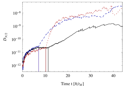
One obvious error source is the one stemming from the discretization of time in order to numerically compute equation (21), so it is necessary to keep the actual time step ${\delta}t$ small enough to have a good approximation of $H(t)$ in the interval $[t,t+{\delta}t]$. But this error source is not inherent to the TEBD implementation. The main error sources in the algorithm are the Suzuki-Trotter approximation and the Schmidt truncation. In order to improve the time step error, one can use higher dimensional Suzuki-Trotter formulas, at a computational cost which scales linearly with higher-order approximationsHatano05 , or we can decrease the time step ${\delta}t$, which also comes at a linear cost $n_{t}=\frac{{\delta}t}{\tau}$. The dominating error in probably all setups of interest is thus the truncation error. It is also very difficult to compensate for this error, because of the $\mathcal{O}({\chi_{c}}^{3})$ scaling of the computational cost. As a trivial example, when starting a real time evolution with a state with Schmidt dimension smaller than $\chi_{c}$, the simulation runs with a constant truncation error. As the simulation continues, there comes a point where more states than $\chi_{c}$ are needed, and the truncation error quickly overcomes the Trotter error, which basically defines a runaway time for the simulation, as reported in Ref. Gobert05, . A reasonable and often used estimator of the truncation error is the discarded weight

$$D_{k}=1-\sum_{\alpha_{k}=1}^{\chi_{m}}\lambda_{\alpha_{k}}^{2}$$ (27)

where $D_{k}$ denotes the discarded weight for a bipartite split at the $k$-th bond and $\chi_{m}<\chi_{c}$ is the number of kept eigenvalues. For our real time simulations, we use a maximal Schmidt dimension in the range of $300\leq\chi_{c}\leq 500$, depending on the specific parameter combination. We use a site-dependent $\chi_{c}(\text{site})$ and allow our simulations to adapt $\chi_{c}(\text{site})$ if test values (discarded weight, von-Neumann entropy) show the necessity to do so. We have to remark that for higher $|V_{\text{H}}|$ and $\Delta\epsilon$ the correlations (and thus the needed Schmidt dimension) within the spinless fermion model grow very quickly. Hence, the chosen $\chi_{c}$-range can lead to significantly larger errors in the regime $|V_{\text{H}}|\geq 1.6t_{\text{H}}$ and $\Delta\epsilon\geq 3t_{\text{H}}$.

Figure 5: Current for non-interacting fermions for setup (I). Shown are TEBD (dots on top of the dashed line) and exact results (dashed and solid lines) obtained with the equation of motion method for the single particle reduced density matrix (13) for different system sizes $N$.

Figure 6: Classical $LC$ line with on-site applied potentials $\phi_{i}$.

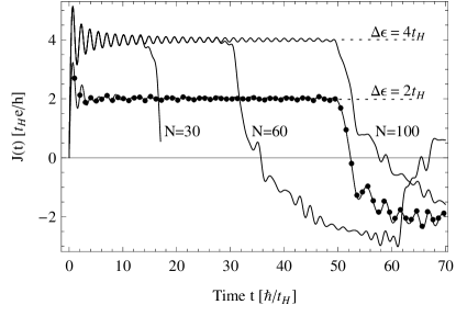
Figure 4 shows the discarded weight for different parameters for a split in the middle of the chain. One can see the runaway time indicated by the vertical lines. However, the maximal discarded weight over all simulations, sites and times up to $40\hbar/t_{\text{H}}$ we measured is yet smaller than $10^{-6}$. Our simulations reveal that when taking a maximal Schmidt dimension of $\chi_{c}=600$ instead of 300, the runaway time is shifted only about 20% to larger times and our quantities of interest are only slightly changed. Moreover, the stationary current computed with our method, which is described later, is only changed by less than 0.5%.

Figure 5 shows the very good agreement between our TEBD simulations and the exact calculation using the single particle reduced density matrix (13) for spinless fermions in the tight-binding model. We use a time step $\delta t=0.01$ and a typical simulation runs approximately 1/2 to 8 hours for a ground state calculation and about 4 hours to (seldomly) 1 week for a real time evolution. We use a multi-threaded version of TEBD with an extremely low overhead (less than 1% for 10 processors and less than 5% for up to 96 processors). The overall cost of a TEBD simulation is slightly higher than that of a DMRG calculation on a single processor. If several processors are used in parallel the overhead of DMRG calculations become rapidly prohibitive, exceeding 100 % for as few as 4 processors.Hager04 Thus TEBD is already twice as fast as DMRG for 4 processors and the difference is likely to increase rapidly with the number of processors. We have used 12 threads for a TEBD simulation on average.

III Classical $LC$ line

In the following, our attention will be put on a classical model: the so-called $LC$ line, shown in Fig. 6. The $LC$ line has been under research as an electrical circuit implementation of a Toda chainHirota73 ; Toda75 ; Singer99 , a nonlinear oscillator chain that, among others, describes the propagation of soliton waves. Further investigations of the $LC$ line have so far been focused on the continuous and linear case.Ingold92 While this setup has therefore been analyzed for the nonlinear and the linear and continuous case, our focus lies on a discrete and linear model for finite and infinite sizes.

In the following, we show that the $LC$ line serves well as the classical representation of a one-dimensional quantum wire described by the tight-binding Hamiltonian, while our main focus lies on the behaviour of the current, especially the influence of finite-size effects and stationary values for the infinite-size limit. We present solutions for a setup in which an initial imbalance of charge carriers on the condensators leads to an oscillating, rectangular current curve as the charge carriers move back and forth in the $LC$ line: the formerly described setup (I). Scaling the system size $N$ to infinity leads to an enlargement of the square wave period, and for large times a stationary current $\bar{I}$ is flowing. Subsequently, a method is presented to compute the stationary current $\bar{I}$ for infinitely large systems using finite-size simulation results. Based on the comparison of the classical and quantum mechanical model this approach will be applied to quantum systems.

Figure 6 shows the classical, electronic setup of a one-dimensional wire that possesses many properties of a one-dimensional quantum chain. This $LC$ line is a combination of condensators and inductors whereas the present model is extended to enable on-site applied potentials $\phi_{i}$. For this setup, the following relations can be derived using elementary electrotechnical relations and Kirchhoff’s laws

$$J_{i} = -C_{i}\dot{U}_{i}\quad;\quad i=1,2,..,N$$

$$V_{i} = L_{i}\dot{I}_{i};\quad i=1,2,..,N-1$$ (28)

$$I_{i+1} = I_{i}+J_{i+1};\quad i=0,1,..,N-1$$

and

$$V_{i}=U_{i}-U_{i+1}+\phi_{i}-\phi_{i+1}\quad;\quad i=1,2,..,N-1$$ (29)

where $I_{0}=I_{N}=0$ was defined. $V_{i}$ in equation (29) results from the potential difference between the left ($\phi_{i}+U_{i}$) and right ($\phi_{i+1}+U_{i+1}$) connection of the $i$-th inductor. $C_{i}$ denotes the capacity of the $i$-th capacitor, $U_{i}$ the voltage drop over the capacitor, $L_{i}$ the inductance of the $i$-th inductor and $I_{i}$ and $J_{i}$ are the currents as shown in Fig. 6. $Q_{i}$ is the charge of the $i$-th capacitor and the $\phi_{i}$ denote externally applied potentials. From the equations above follows

$$\ddot{\vec{I}}=-M\vec{I}+\dot{\vec{\Phi}}$$ (30)

with

$$M_{ij}= - \delta_{i,j+1}\left(\frac{1}{L_{i}C_{i}}\right)-\delta_{i,j-1}\left(\frac{1}{L_{i}C_{i+1}}\right)$$ (31)

$$+ \delta_{ij}\left(\frac{1}{L_{i}C_{i+1}}+\frac{1}{L_{i}C_{i}}\right)$$

and $\dot{\Phi}_{i}=(\dot{\phi}_{i}-\dot{\phi}_{i+1})/L_{i}$. We consider an $LC$ line with equal capacities and inductances

$$L_{i}=L\quad\text{and}\quad C_{i}=C\quad\forall i$$ (32)

and temporally constant applied potentials $\dot{\vec{\Phi}}=\vec{0}$ for which it follows

$$I_{i}(t)=\sqrt{\frac{2}{N}}\sum_{k=1}^{N-1}\sin\left(\frac{ki\pi}{N}\right)\left[b_{k}\sin\left(\omega_{k}t\right)+d_{k}\cos\left(\omega_{k}t\right)\right]$$ (33)

and

$$\omega_{k}=\frac{2}{\sqrt{LC}}\sin\left(\frac{k\pi}{2N}\right).$$ (34)

With $Q_{0,i}:=Q_{i}(t=0)$ and $\phi_{0,i}:=\phi_{i}(t=0)$ one has

$$\dot{I}_{i}(0)=\frac{1}{LC}\left(Q_{0,i}-Q_{0,i+1}\right)+\frac{1}{L}\left(\phi_{0,i}-\phi_{0,i+1}\right)$$ (35)

and thus

$$b_{k} = \frac{\sqrt{2}}{\omega_{k}L\sqrt{N}}\sum_{i=1}^{N-1}\left[\frac{1}{C}(Q_{0,i}-Q_{0,i+1})\right.$$ (36)

$$\quad\quad\left.\phantom{\frac{|}{|}}+\phi_{0,i}-\phi_{0,i+1}\right]\sin\left(\frac{ki\pi}{N}\right).$$

III.1 Stationary current

In the following, we assume that initially (at $t=0$) no current is flowing

$$I_{i}(0)=0\quad\forall i\quad\Rightarrow\quad d_{k}=0\quad\forall k$$ (37)

and that the chain is divided into two halves in which the charge carriers are uniformly distributed, i.e.

$$Q_{L}=Q_{0,i=1,..,\frac{N}{2}}\quad,\quad Q_{R}=Q_{0,i=\frac{N}{2}+1,..,N}$$

and $$\phi_{i}(t)=0\quad\forall i,t,$$ (38)

which corresponds to the previously mentioned setup (I).

Figure 7: Current $I_{250}(t)$ for a classical wire of size $N=500$ through the inductor at position $N/2$. $L=C=1$, $Q_{L}=Q_{0,i\leq N/2}=1$ and $Q_{R}=Q_{0,i>N/2}=-1$

Figure 7 shows the current through the inductor $L_{N/2}$ according to the general formula for the current at site $N/2$ for any even $N$

$$I_{N/2}(t)=\frac{Q_{L}-Q_{R}}{N\sqrt{LC}}\sum_{k=1}^{N/2}\frac{\sin\left(\frac{2}{\sqrt{LC}}\eta_{k}t\right)}{\eta_{k}}$$ (39)

with

$$\eta_{k}=\omega_{2k-1}\frac{\sqrt{LC}}{2}=\sin\left(\frac{(2k-1)\pi}{2N}\right).$$ (40)

All values for the classical system ($Q_{i}$, $t$, $L$, $C$, etc.) are given in S.I. units unless otherwise specified.

While the rectangular shape of the dominant oscillation is understandable through the picture of charge carriers moving back and forth in the line, the rapid oscillation on top of the square wave is harder to explain and we will later take a closer look at it. The period $T^{\text{max}}_{\text{cl}}$ of the square wave can be calculated by using equation (39) and (40) and taking only the smallest frequency into account

$$T^{\text{max}}_{\text{cl}}=\frac{\pi\sqrt{LC}}{\sin\left(\frac{\pi}{2N}\right)}.$$ (41)

For large system sizes ($N\gg 1$) this period is approximately given by

$$T^{\text{max}}_{\text{cl}}\approx 2N\sqrt{LC}$$ (42)

and is thus linearly dependent on $N$. In the second half period of the current in Fig. 7 one can see a beat upon the rapid oscillation. This is due to the unequally distributed charges which form an oscillating pattern and so create additional frequencies in the current. This effect also occurs in quantum wires, not only after the reflection at the right border but already from the beginning due to using an initial (ground) state with non-uniform local densities.

In contrast to the oscillating current in a finite system where the charge carriers are scattered at the borders, we assume that the current in an infinitely large system is constantly flowing in one direction. To validate this assumption one has to execute the limit $N\rightarrow\infty$ first, and then take the limit $t\rightarrow\infty$. In the limit $N\rightarrow\infty$ one gets from equation (39)

$$I_{\infty}(t) = \lim_{N\rightarrow\infty}I_{N/2}(t)$$ (43)

$$= \frac{Q_{L}-Q_{R}}{\sqrt{LC}}\frac{1}{\pi}\int_{0}^{1}\frac{\sin\left(a\xi\right)}{\xi\sqrt{1-\xi^{2}}}d\xi$$

with $a=2t/\sqrt{LC}$ and $\varphi=2/\sqrt{LC}$. The solution is given by

$$I_{\infty}(t) = \frac{\left(Q_{L}-Q_{R}\right)t}{2LC}\bigl{[}\mathcal{J}_{0}\left(\varphi t\right)\left(2-\pi\mathcal{H}_{1}\left(\varphi t\right)\right)$$ (44)

$$\quad\quad+~{}\pi\mathcal{J}_{1}\left(\varphi t\right)\mathcal{H}_{0}\left(\varphi t\right)\bigr{]}$$

where $\mathcal{J}_{n}(x)$ are the Bessel functions of the first kind and $\mathcal{H}_{n}(x)$ denote the Struve functions.Abramowitz72

Figure 8: Solid curve: Current $I_{\infty}(t)$ for a classical infinite wire through the inductor at the middle with $L=C=1$, $Q_{L}=1$ and $Q_{R}=-1$. The dashed curve is the current for a finite system with size $N=30$. The constant line denotes the stationary value $1$ against which the solid line converges.

The current for the infinite system (44) is shown in Fig. 8 and it shows that for smaller times the curve for finite system sizes matches the one for the infinitely large LC line. Hence, a very accurate approximation of the value of a stationary current in an infinitely large system can be extracted from the value of a corresponding finite system result. This behaviour will be later used for the analysis of quantum systems.

Using the approximations (A) for the Bessel and Struve functions we find the value of the stationary current in the infinitely large system

$$\bar{I}_{\text{cl}}=\lim_{t\rightarrow\infty}I_{\infty}(t)=\frac{Q_{L}-Q_{R}}{2\sqrt{LC}}.$$ (45)

The conductance $G_{\text{cl}}$ for the stationary case is given by

$$G_{\text{cl}}=\frac{\bar{I}_{\text{cl}}}{V}=\frac{1}{2}\sqrt{\frac{C}{L}}$$ (46)

with a local voltage drop $V=\left(Q_{L}-Q_{R}\right)/C$ in the middle of the chain.

III.2 Finite-time and finite-size effects

In order to describe finite-time effects in the infinite system we seek for a simpler current expression which does not only give the correct stationary value but also a good approximation for the short-time behaviour. Using the asymptotic series expansions (A), $I_{\infty}(t)$ can be transformed into the following form for $t\gg 1$

$$I_{\text{app}}(t) =\bar{I}_{\text{cl}} +I_{\text{dev}}(t)$$ (47)

$$=\bar{I}_{\text{cl}} +\frac{Q_{L}-Q_{R}}{16}\sqrt{\frac{\varphi}{\pi t}}\bigl{[}(10\pi-32)(\sin^{2}(\varphi t)$$

$$+~{}\sin(\varphi t)\cos(\varphi t))$$

$$+~{}4(\sin(\varphi t)-\cos(\varphi t))\bigr{]}+\mathcal{O}\left(\frac{1}{t}\right)$$

with $\varphi=2/\sqrt{LC}$. $I_{\text{dev}}(t)$ denotes the deviation from the stationary current $\bar{I}_{\text{cl}}$ from equation (45). The order $\mathcal{O}\left(t^{-1}\right)$ of the rest term is only valid if the approximation of $\mathcal{H}_{1}(x)$ in (A) has an error of smaller order which presumably holds according to Ref. Aarts03, .

Figure 9: Exact current $I_{\infty}(t)$ (solid line) and approximative current $I_{\text{app}}(t)$ (dashed line) with $L=C=1$, $Q_{L}=1$ and $Q_{R}=-1$.

As shown in Fig. 9, expression (47) is a pursuasive approximation even for smaller times and thus a good explanatory basis for short-time effects in the $LC$ line. It states a general $\mathcal{O}(1/\sqrt{t})$ decay of the amplitudes of the rapid oscillation in the current curve which is the maximal order of the error for an approximation of the stationary current (45) using a finite-time (i.e. a finite-size) result.

Instead of looking at the current through a single inductor, one can consider the current through two or more neighbouring ones. We will show that the short time behaviour of this current has some advantages compared to the simple $I_{N/2}(t)$ curve. We define the quantity of interest for even $N$ as

$$I_{\text{m,}N/2}(t)=\frac{1}{2}I_{N/2}(t)+\frac{1}{4}\left(I_{N/2+1}(t)+I_{N/2-1}(t)\right)$$ (48)

which is equal to the expression $\frac{1}{2}(I_{N/2}(t)+I_{N/2+1}(t))$, whereas for the latter expression the subsequently explained effect also occurs for odd $N$ for the substitution $N/2\rightarrow(N-1)/2$. In the limit $N\rightarrow\infty,t\rightarrow\infty$, $I_{\text{m,}N/2}(t)$ converges against the same value as $I_{N/2}(t)$ which implies that the stationary current is as well assessable via the current through two or more adjacent inductors. From (33) one gets

$$I_{\text{m,}N/2}(t) = \frac{Q_{L}-Q_{R}}{NLC}\sum_{k=1}^{N-1}\frac{1}{\omega_{k}}\sin\left(\omega_{k}t\right)\sin^{2}\left(\frac{k\pi}{2}\right)$$ (49)

$$\cdot\left[1+\cos\left(\frac{k\pi}{N}\right)\right]$$

with expression (36) for $b_{k}$ and the step distribution for the charges (III.1). In the limit $N\rightarrow\infty$ it follows

$$I_{\text{m,}\infty}(t)=\frac{Q_{L}-Q_{R}}{\pi\sqrt{LC}}\int_{0}^{\frac{\pi}{2}}\frac{\sin\left(\frac{2}{\sqrt{LC}}\sin\left(x\right)t\right)}{\sin\left(x\right)}\cos^{2}(x)dx.$$ (50)

The integral can be solved in analogy to (43) with the substitution $\xi=\sin\left(x\right)$ and gives

$$I_{\text{m,}\infty}(t) = \frac{Q_{L}-Q_{R}}{\sqrt{LC}}\left[\mathcal{J}_{1}(\varphi t)\left(\frac{\pi\varphi t}{4}\mathcal{H}_{0}(\varphi t)-\frac{1}{\varphi^{2}t^{2}}-\frac{1}{2}\right)\right.$$ (51)

$$+~{}\left.\mathcal{J}_{0}(\varphi t)\left(\frac{\varphi t}{2}+\frac{1}{2\varphi t}-\frac{\pi\varphi t}{4}\mathcal{H}_{1}(\varphi t)\right)\right].$$

Figure 10: Solid curve: Current $I_{\text{m,}\infty}(t)$ through two adjacent inductors in the middle; equation (51). Dashed curve: Current $I_{\infty}(t)$ from equation (44) through a single inductor. $L=C=1$, $Q_{L}=1$ and $Q_{R}=-1$.

This result, plotted in Fig. 10 together with equation (44) for the current $I_{\infty}(t)$ through a single inductor, shows almost no rapid oscillations. An approximative expression for the rapid oscillations $I_{\text{r}}(t)\approx I_{\text{dev}}(t)$ can therefore be derived using the difference between the two current expressions (51) and (44)

$$I_{\text{r}}(t) = I_{\text{m,}\infty}(t)-I_{\infty}(t)$$ (52)

$$= \frac{Q_{L}-Q_{R}}{4}\left[\frac{\mathcal{J}_{0}(\varphi t)}{t}-\left(\frac{2}{\varphi t^{2}}+\varphi\right)\mathcal{J}_{1}(\varphi t)\right]$$

and using the approximations (A) for the remaining Bessel functions one has

$$I_{\text{r,app}}(t) = \frac{(Q_{L}-Q_{R})}{32\sqrt{\pi}\left(\varphi t\right)^{5/2}t}\left[\left(5(\varphi t)^{2}+8(\varphi t)^{3}\right.\right.$$ (53)

$$\left.\left.+~{}15\varphi t-6\right)\cos(\varphi t)\left(5(\varphi t)^{2}-8(\varphi t)^{3}\right.\right.$$

$$\left.\left.-~{}15\varphi t-6\right)\sin(\varphi t)\right].$$

Hence the rapid oscillations have a radial frequency $\varphi=2/\sqrt{LC}=2\pi/T^{\text{min}}_{\text{cl}}$ and thus

$$T^{\text{min}}_{\text{cl}}=\pi\sqrt{LC}.$$ (54)

III.3 Determining the stationary current from finite system values

There are various methods to calculate the stationary current from simulation results stemming from systems with finite size. The most obvious and easiest way to do so is to use the curve of a current through the middle inductor (or the mean value of currents through two or more adjacent inductors) and to compute the mean value over a certain time interval in the quasi-stationary regime. In contrast to this approach, we will present a more analytical approach using the Fourier transformation. Although one cannot prove that the following strategy can be applied to quantum mechanical systems with complicated interactions, several numerical and theoretical indications are given in sections IV and V. We start with a square wave described by its Fourier series

$$\mathcal{R}_{m}(t):=\frac{4A}{\pi}\sum_{k=1}^{m}\frac{\sin\left((2k-1)\chi t\right)}{2k-1}$$ (55)

where $m$ determines the number of harmonics, $A$ denotes the value of the quasi-stationary plateau and $\chi=2\pi/T^{\text{max}}_{R}$ where $T^{\text{max}}_{R}$ is the period of the square wave. This signal has certain similarities with the current curve $I_{N/2}(t)$. It possesses a quasi-stationary regime which becomes infinite for $\chi\rightarrow 0$ (equals $N\rightarrow\infty$ for the $LC$ line) and shows a rapid and decaying oscillation on top of it. The main difference between the composition of the current curve (39) and the square wave is the presence of sine-functions that enclose the $(2k-1)$-terms.

The current in (39) is dependent on $\eta_{k}$ and it is thus convenient to write $I_{N/2}^{[\eta_{k}]}(t)$ where $\eta_{k}=\sin(\frac{(2k-1)\pi}{2N})$. Choosing an $\eta_{k}$ without the enclosing sine-functions gives

$$I_{N/2}^{\left[\frac{(2k-1)\pi}{2N}\right]}(t)=\frac{2(Q_{L}-Q_{R})}{\pi\sqrt{LC}}\sum_{k=1}^{N/2}\frac{\sin\left((2k-1)\varphi^{\prime}t\right)}{2k-1}$$ (56)

with $\varphi^{\prime}=\varphi\pi/(2N)=\pi/(N\sqrt{LC})$. Since expression (56) now describes a square wave, one can compare it with (55) and get its quasi-stationary value

$$A=\frac{Q_{L}-Q_{R}}{2\sqrt{LC}}=\bar{I}_{\text{cl}}$$ (57)

which is equal to the value that was derived for the stationary current in equation (45). Remarkably the enclosing sine-functions do not change the stationary value, i.e. the expression (56) and the current in an $LC$ line have the same stationary value for $N\rightarrow\infty$. In case of expression (56) this value is equal to the quasi-stationary value (57) which leads to the idea to calculate the quasi-stationary value from a given current signal in a finite system (using the procedure described below) and use it as approximation for the stationary current value for $N\rightarrow\infty$.

Applying the Fourier-transformation

$$\tilde{I}_{N/2}(\omega):=\int_{-\infty}^{\infty}I_{N/2}(t)e^{i\omega t}dt$$ (58)

term by term to expression (39) gives

$$\tilde{I}_{N/2}(\omega)=i\cdot\frac{(Q_{L}-Q_{R})}{N\sqrt{LC}}\sum_{k=1}^{N/2}\frac{\delta(\omega+\varphi\eta_{k})-\delta(\omega-\varphi\eta_{k})}{\eta_{k}}$$ (59)

with equation (40) for $\eta_{k}$ and $\varphi=2/\sqrt{LC}$. If numerical data with $m$ values are given, one can only apply a discrete Fourier transformation which preserves the area underneath a delta peak, such that for any interval $\Delta t$ containing a single delta function $a\cdot\delta(x-x_{0})$ the peak is of height $a/\Delta t$. Taking only the first ($k=1$) and only the positive delta-peak into account and using the discrete transformation

$$\tilde{f}(j)=\frac{1}{m}\sum_{k=0}^{m-1}f(k)e^{-ikj\omega_{0}}\quad\phantom{=}\text{with}\phantom{=}\omega_{0}=\frac{2\pi}{m}$$ (60)

and $j=0,1,...,m-1$, one gets for the current

$$\bar{I}_{\text{cl}}=\frac{\text{Im}[\tilde{I}_{N/2}(\omega_{1})]N\Delta t}{2}\cdot\sin\left(\frac{\pi}{2N}\right)$$ (61)

where $\text{Im}[\tilde{I}_{N/2}(\omega_{1})]$ is the height of the first discrete peak ($k=1$). In fact, one cannot expect to know the precise form of $\eta_{k}$ for complicated quantum systems. Instead, one can take a first order approximative expression. For $N\gg 1$ it holds $\sin\left(\frac{\pi}{2N}\right)\approx\frac{\pi}{2N}$, which implies that the given curve is a square wave, and thus

$$\bar{I}_{\text{cl}}\approx\frac{\pi}{4}\text{Im}[\tilde{I}_{N/2}(\omega_{1})]\Delta t$$ (62)

with a relative errorAbramowitz72

$$\frac{|\Delta\bar{I}_{\text{cl}}|}{|\bar{I}_{\text{cl}}|}\leq\frac{\pi^{2}}{8N^{2}}.$$ (63)

It is important to remark that equation (62) is not only an exact result for a square wave, but also an excellent approximation for the $LC$ line current with maximal error according to equation (63).

As our simulations reveal, the charge carriers in the $LC$ line coming from the left half first reach the right border at $t\approx T^{\text{max}}_{\text{cl}}/4$. After this time the finite system size has a significant influence on the simulation results. Applying a discrete Fourier transformation means to assume that a periodic function is given. For that, and to minimize the upcoming error for times larger than $T^{\text{max}}_{\text{cl}}/4$ the following procedure is proposed: From a given current curve $I_{N/2}(t)$ stemming from simulation results, first determine a position $t=t_{s}$ in the vicinity of $T^{\text{max}}_{\text{cl}}/4$ – but smaller than $T^{\text{max}}_{\text{cl}}/4$ – where the curve could be mirrored along a parallel to the $y$-axis such that the loss of continuity is minimized, which is the case for instance at inflection points. Then consider a $4t_{s}$-periodic function, constructed as follows

$$I_{\mathcal{R}}(t,t_{s}):=\left\{\begin{array}[]{c c}I_{N/2}(t)\phantom{2t_{s}.....}&\text{for }0\leq t<t_{s}\phantom{+..}\\ I_{N/2}(2t_{s}-t)&\text{for }t_{s}\leq t<2t_{s}\phantom{.,}\\ -I_{N/2}(t-2t_{s})&\text{for }2t_{s}\leq t<3t_{s}\\ -I_{N/2}(4t_{s}-t)&\text{for }3t_{s}\leq t\leq 4t_{s}\end{array}\right..$$ (64)

We then apply the Fourier transformation to the constructed signal (64) and use equation (62) to calculate the corresponding stationary value of the current, see Fig.  11.

Figure 11: Constructed signal $I_{\mathcal{R}}(t,t_{s})$ from simulation results together with the Fourier series representation of a square wave $\mathcal{R}_{m}(t)$ from (55) with $m=8$ and an ideal square wave $R(t)$. The Fourier transformation of $I_{\mathcal{R}}(t,t_{s})$ and expression (62) was used to calculate the amplitude of $R(t)$.

III.4 A final note on setups

Instead of initially dividing the system into two halves with different charges $Q_{L}$ and $Q_{R}$, we can distribute the charge carriers homogeneously over the chain, apply a temporally constant voltage ($\phi_{0,L}-\phi_{0,R}$) and get the same result for the current as a function of time, which can be seen in equation (36) for $b_{k}$. The reason for this lies in the linear character of our model which is as a consequence independent from the chosen setup. This is the main reason why we cannot fully compare the $LC$ line with a quantum system, since preparing the classical system in setup (II) gives the same outcomes as for setup (I), in contrast to our quantum simulation results.

IV Finite-size effects and stationary current in quantum systems

IV.1 Finite-size induced oscillation

Figure 12: Current in the tight-binding model for a long time scale, calculated using the one-particle equation of motion. The initial state was prepared with a completely filled left half, a completely empty right half and $t_{\text{H}}=0$ for all bonds.

With both setups (I) and (II) one observes qualitatively similar currents in the tight-binding model (the spinless fermion model without interaction $V_{\text{H}}=0$) as a function of time, as shown in Figs. 5 and 12. First, there is a small transient regime for $t<t_{a}\lesssim 3h/t_{\text{H}}$ with very rapid and dominant small oscillations. For long times $t>t_{b}\gg T^{\text{max}}$ the current becomes very irregular because of the progressive dephasing of moving particles. Between $t_{a}$ and $t_{b}$ we observe an approximately rectangular wave with a period $T^{\text{max}}$ which diverges with increasing system length (the corresponding leading frequency $\omega^{\text{max}}=2\pi/T^{\text{max}}$ converges towards 0 in the thermodynamic limit), see Fig. 12. The period of the rectangular oscillation is given by (Appendix B)

$$T^{\text{max}}\approx\hbar\cdot\frac{N}{t_{\text{H}}}\quad\text{for}\quad N\gg 1.$$ (65)

For spinless fermions, using a semi-classical picture, particles first flow from one side of the system to the opposite side because of the inhomogeneous density (first setup) or the potential difference (second setup). Then they are reflected by the hard wall represented by the chain edge. As there is no dissipation in our model, all reflected particles flow back with the same velocity in the opposite direction until they reach the other chain edge and are again reflected and so on.

The progressive degradation of the rectangular signal can be understood using the same picture. First, all particles flow in the same direction but, as they have different velocities, they progressively come out of phase. For long times $t\gg t_{b}$, which can be checked up to the numerical double limit $t\approx 10^{300}$ for non-interacting fermions ($V_{\text{H}}=0$), our simulations show that the current does not go to zero but continues to oscillate with a period $T^{\text{max}}$. This can be understood in the picture of the classical $LC$ line as well as for spinless fermions through the dominant amplitude of the $\omega^{\text{max}}$ oscillation. It is basically the same effect as if all contributions to a series representation of a square wave (55) would ‘randomly’ come out of phase. In that case, the contribution with the lowest frequency $\omega^{\text{max}}$, which is the frequency of the rectangular oscillation, determines the frequency of the remaining irregularly shaped curve.

IV.2 Rapid oscillation on top of the square wave

Figure 13: Current in the tight-binding model for $\Delta\epsilon=2t_{\text{H}}$, calculated using the one-particle equation of motion. The dashed lines are currents through a single bond in the chain while the solid ones represent the mean value of the currents through two adjacent bonds in the middle.

Setting the two expressions (41) and (65) for the periods of the classical and quantum mechanical system equal one gets

$$t_{\text{H}}\approx\frac{\hbar}{2\sqrt{LC}}\quad\text{for }N\gg 1.$$ (66)

Further comparison with equation (54) gives for the period of the rapid oscillation

$$T^{\text{min}}=\pi\sqrt{LC}\approx\frac{h}{4t_{\text{H}}}\quad\text{for }N\gg 1.$$ (67)

Instead of preparing the system in a ground state of a Hamiltonian with applied potentials, one can initially decouple all sites and fill the left half of the system with (uncorrelated) particles, leaving the right half empty. This almost corresponds to choosing $\Delta\epsilon=4t_{\text{H}}$, insofar as a ground state with this applied voltage and coupled reservoirs still has some correlations and unequally distributed on-site particle densities in it. The resulting current curve in Fig. 12 in the first half period closely resembles the curve shown in Fig. 7 for the $LC$ line.

The magnification in Fig. 12 shows a rapid oscillation with a period according to equation (67), in contrast to the oscillation shown in Fig. 13 for setup (I) which is ‘disturbed’ by oscillations stemming from correlations and an unequal distribution of particles in the ground state due to a lower applied voltage $\Delta\epsilon<4t_{\text{H}}$. Although the oscillation in Fig. 13 for setup (II) is very regular, it does not stem from the same ‘classical’ origin, which is confirmed by the fact that on the one hand two adjacent currents do not cancel out and on the other hand the oscillation does not fulfill equation (67).

Since in the following we are more interested in the stationary current flowing from an infinitely large source (the left half of the chain) to a an infinitely large drain (the other half), we reference to Ref. Wingreen93, for a discussion of time-dependent currents and to Ref. Branschaedel10, for a detailed analysis of short-time and finite-size effects (in the IRLM).

IV.3 Applicability of the extrapolation approach to quantum systems

Although we have seen the close connection between the tight-binding system for initially uncorrelated particles and the classical $LC$ line, there exists a major difference in the behaviour of the respective currents: the damping of the rapid oscillations. While for the classical $LC$ line a $\mathcal{O}(t^{-\frac{1}{2}})$ dependence of the amplitudes according to equation (47) is predicted, this decrement is different for a quantum system.

Figure 14: Solid line: $J_{\text{F}}(t)$ from equation (68), dashed line: corresponding approximation $J_{\text{F,app}}(t)$ from (69).

The expectation value of the current for setup (I) and for initial conditions like in Fig. 12 (one completely filled and one completely empty half) is for $N\rightarrow\infty$ given byAntal99 ; Hunyadi04 (Appendix C)

$$J_{\text{F}}(t)=\frac{et_{\text{H}}}{\hbar}\omega t\left[(\mathcal{J}_{0}(\omega t))^{2}+(\mathcal{J}_{1}(\omega t))^{2}\right].$$ (68)

with $\omega=2t_{\text{H}}/\hbar$. Using the asymptotic series expansions (A) yields for the current

$$J_{\text{F,app}}(t) = \frac{et_{\text{H}}}{16h(\omega t)^{2}}\bigl{[}5-32\omega t\cos(2\omega t)$$ (69)

$$+~{}4\sin(2\omega t)\bigr{]}+\frac{4et_{\text{H}}}{h}$$

which is plotted together with expression (68) in Fig. 14.

The curve highly coincides with the one shown in Fig. 12 for $t<T^{\text{max}}/4$ which confirms the assumption that the borders in the finite quantum system for setup (1) only significantly change the current after a time $T^{\text{max}}/4$, determined by the velocity of the particle density front waveHunyadi04 which moves from the middle of the chain to the borders. The quasi-stationary value $\bar{J}=4et_{\text{H}}/h$ from (69) suits equation (10) for $\Delta\epsilon=4t_{\text{H}}$ and the amplitudes of the rapid oscillation are damped with $\mathcal{O}(1/t)$. Moreover, expression (67) for the period of the rapid oscillation – which was derived only by comparison with the classical model – is confirmed by equation (69).

Since the latter analysis shows a $\mathcal{O}(1/t)$ damping of the rapid oscillation, the open question at hand is, if it is reasonable to use our extrapolation method for a quantum system. In fact, a pure square wave described by its Fourier series (55) has also a damping of the rapid oscillation of $\mathcal{O}(1/t)$ and highly resembles the current described by (68) or depicted in Fig. 12 when choosing an appropriate amplitude and number of harmonics. Since the mathematical error (63) of our method stems from the difference of the analyzed curve to a square wave, the extrapolation approach provides an even smaller error than (63) for a quantum system.

V Spinless fermion model

In this section we discuss our results for the stationary current and the finite-system period in the spinless fermion model. The non-linear dynamics of this model and the closely related spin $\frac{1}{2}$ $XXZ$ chain have been studied in several works using td-DMRG methods Schmitteckert04 ; Gobert05 ; Langer09 . Nevertheless, the steady-state transport properties of the spinless fermion model have not been investigated yet.

V.1 Current-voltage characteristics

Firstly, we remark that the value of the potential bias is given by the parameter $\Delta\epsilon$ of the Hamiltonian from equation (4), and it is not the result of a quantum measurement of an observable. Thus it corresponds to an external field applied to the system, and in an interacting system it is not always equal to the actual potential difference which is measured in experiments.Kawabata07 ; Kawabata96 Moreover, in experiments the sample (quantum wire) must be connected by leads to the voltage source and measurement apparatus. This modifies the low-energy, low-temperature behaviour of the sample below some crossover energy scale.Kane92 ; Safi95 Concerning this matter, the linear conductance of a TLL attached to one-dimensional leads has been calculated in several works.Safi95 ; Maslov95 ; Ponomarenko95 ; Janzen06 It has been shown that the conductance of this setup is given by $e^{2}/h$ (which corresponds to equation (10) with $K=1$), independently of the Coulomb interaction $V_{\text{H}}$ within the wire, and that this result coincides with experimental outcomes.

Our analysis of on-site particle densities shows that the densities for the first and last site of the chain only change after $T^{\text{max}}/4$. This is a major reason why we only take values of the current for times smaller than $T^{\text{max}}/4$ into account, as described in our extrapolation approach. To test the overall procedure for computing the stationary current we have first calculated the current-voltage characteristic of a non-interacting chain ($V_{\text{H}}=0$). This characteristic is known exactly for the first setupAntal99 ; Hunyadi04 : $\bar{J}=(e/h)\Delta\epsilon$ for $|eV|\leq 4t_{\text{H}}$ and $\bar{J}=(e/h)4t_{\text{H}}$ for $|eV|\geq 4t_{\text{H}}$, with $\Delta\epsilon=|eV|$ where $V$ is the voltage bias. For the second setup, exact results were calculated numerically using the one-particle equation of motion with a system size of $N=1000$.

We have found that our procedure yields stationary current values which agree with an overall error of less than 5% with the exact results. As a second test we have calculated the current-voltage characteristic of the IRLM. The generic shape of this curve is known from a field-theoretical analysis, and highly accurate td-DMRG results are available for a quantitative comparison.Boulat08 In that regard, we have found that the results from our method agree very well with the numerical outcomes from Ref. Boulat08, . We nevertheless have to remark that we found the IRLM far easier to simulate than the spinless fermion model, since for higher $|V_{\text{H}}|$ the correlations (and thus the needed Schmidt dimension) within the spinless fermion model grow more quickly than in the IRLM. As already mentioned in section II.4 the parameters used for our simulations can result in larger errors for high voltages and Coulomb interactions in the TEBD data for the current as a function of time. Additionally, finite-size effects also grow with $|V_{\text{H}}|$ and $\Delta\epsilon$. This can lead to less accurate extrapolations for the steady-state current in that regime than for non-interacting fermions and the IRLM.

Figure 15: (Color online) Current-voltage curve of the spinless fermion model with setup (I) for several positive $V_{\text{H}}$. For $V_{\text{H}}=0$ the current has been computed using TEBD and the one-particle equation of motion (eom). The lines are guides for the eyes.

Figure 16: (Color online) Magnification of figure 15. The lines indicate the linear response according to the TLL theory (10) for small $\Delta\epsilon$.

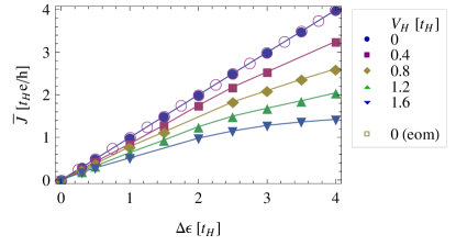
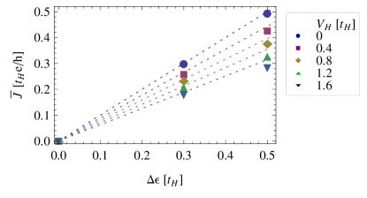
We now discuss the current-voltage characteristics which have been obtained with the methods described above. In setup (I) the current of the non-interacting system ($V_{\text{H}}=0$) is strictly proportional to $\Delta\epsilon=|eV|$ up to the band width $4t_{\text{H}}$ and then remains constant.Antal99 ; Hunyadi04 For $V_{\text{H}}>0$ we see in Fig. 15 that the current increases sub linearly with $\Delta\epsilon$ for a fixed interaction strength $V_{\text{H}}$ and that it decreases monotonically with increasing $V_{\text{H}}$ for a fixed potential bias $\Delta\epsilon$. The magnification in Fig. 16 shows a comparison with the linear response in the TLL theory (10) for small $\Delta\epsilon$, using the Bethe Ansatz solution parameters (3). The good agreement confirms the validity of our approach. Obviously, an increasing $V_{\text{H}}$ does not only reduce the current but also the range of the potential bias $\Delta\epsilon$ for which the linear response approximation is accurate.

Figure 17: (Color online) Current-voltage curve of the spinless fermion model with setup (I) for several negative $V_{\text{H}}$. The dashed lines indicate the theoretical beginning of the current plateaus according to (70). The solid lines are guides for the eyes.

Figure 18: (Color online) Magnification of Fig. 17. The lines indicate the linear response according to the TLL theory (10) for small $\Delta\epsilon$.

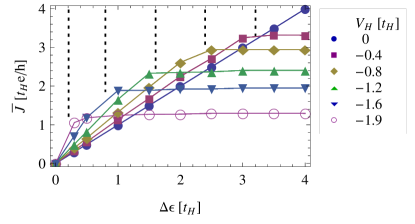
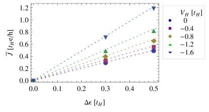
In Fig. 17 we observe a behaviour for attractive interactions $V_{\text{H}}<0$ which is similar to the non-interacting case. The current increases almost linearly with $\Delta\epsilon$ up to some $V_{\text{H}}$-dependent threshold potential where it saturates at its maximal value. Increasing $|V_{\text{H}}|$ scales the maximal current down but causes a higher linear conductance for small $\Delta\epsilon$. Figure 18 shows that for negative interactions there is also an excellent agreement between our results and the linear response in the TLL theory (10) for small $\Delta\epsilon$. Again increasing $|V_{\text{H}}|$ seems to reduce the range of the potential bias $\Delta\epsilon$ for which the linear response approximation is accurate.

The occurrence of current plateaus for large potential differences can be easily understood. In setup (I) one half of the chain initially contains more particles than the other one due to the applied potential bias $\Delta\epsilon$. When this bias is large enough the initial state consists of one completely filled and one completely empty half and it does not change for higher $\Delta\epsilon$. In the non-interacting case this saturation occurs exactly at $\Delta\epsilon=4t_{\text{H}}$.Antal99 ; Hunyadi04 When we add an attractive interaction $V_{\text{H}}<0$ the particles are more likely to stick together and therefore even more particles gather in one half for the same applied potential. Thus, saturation (i.e., an initial state with one completely filled and one completely empty half) is reached for smaller $\Delta\epsilon$ as $|V_{\text{H}}|$ increases as seen in Fig. 17. We do not understand yet why the plateau heights (i.e. the maximal current) are lowered by increasing $|V_{\text{H}}|$. For a repulsive interaction $V_{\text{H}}$ the effect is reversed and less particles gather in one half of the chain for a given potential difference when $V_{H}$ increases. Thus we expect that saturation occurs at higher values $\Delta\epsilon>4t_{\text{H}}$ beyond the potential range shown in Fig. 15. We can easily determine for which potential difference $\Delta\epsilon$ saturation occurs. Removing a single particle from the completely filled reservoir or adding one particle to the empty half costs an energy $\Delta\varepsilon/2-V_{\text{H}}-2t_{H}$. Thus saturation occurs if

$$\Delta\varepsilon\geq 2V_{\text{H}}+4t_{H}.$$ (70)

Figure 17 shows that this approximation fits well to the numercial data for $V_{\text{H}}\leq 0$ whereas the saturated regime according to (70) for $V_{\text{H}}>0$ lies outside the potential range shown in Fig. 15, as mentioned above.

Figure 19: (Color online) Current-voltage curve of the spinless fermion model with setup (II) for several positive $V_{\text{H}}$. For $V_{\text{H}}=0$ the current has been computed using TEBD and the one-particle equation of motion (eom). The lines are guides for the eyes.

Figure 20: (Color online) Magnification of Fig. 19. The lines indicate the linear response according to the TLL theory (10) for small $\Delta\epsilon$.

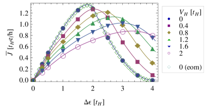
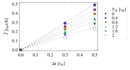
While for setup (I) the differential conductance is always positive (or zero after saturation), in setup (II) we observe a negative differential conductance. Figure 19 shows our results for setup (II) with $V_{\text{H}}\geq 0$. The current seems to vanish for very large potential biases as predicted by strong-coupling perturbation theory for this setup. We note that the current becomes systematically weaker with increasing $V_{\text{H}}$ for a fixed small potential bias. For larger $\Delta\epsilon$ the behaviour of $I$ as a function of $V_{\text{H}}$ is no longer monotonic. In addition, we see that the onset of the negative differential conductance (i.e., the position of the maximum of $I$ as a function of $\Delta\epsilon$) shifts to higher values with increasing $V_{\text{H}}$. The magnification for small $\Delta\epsilon$, Fig. 20, confirms again that our results agree with the TLL theory in the linear regime and that the range of the linear response regime shrinks with increasing interaction strength.

Figure 21: (Color online) Current-voltage curve of the spinless fermion model with setup (II) for several negative $V_{\text{H}}$. The lines are guides for the eyes.

Figure 22: (Color online) Magnification of Fig. 21. The lines indicate the linear response according to the TLL theory (10) for small $\Delta\epsilon$.

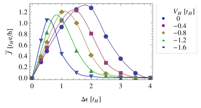
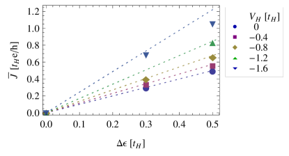
Results for attractive interactions $V_{\text{H}}<0$ are shown in Fig. 21. There we clearly observe that the current vanishes for large potential differences as predicted by strong-coupling perturbation theory for setup (II). We also see that the current becomes systematically larger with increasing interaction strength $|V_{\text{H}}|$ for a fixed small potential bias. For intermediate $\Delta\epsilon$ the behaviour of $I$ as a function of $V_{\text{H}}$ is not monotonic and for large enough $\Delta\epsilon\gtrsim 2t_{\text{H}}$ the current decreases systematically with increasing interaction strength. Moreover, we see that the onset of the negative differential conductance occurs at lower values of $\Delta\epsilon$ for increasing $|V_{\text{H}}|$. Finally, Fig. 22 shows that in this case our results also agree with the TLL theory in the linear regime, but it seems that the interaction reduces rapidly the range of potential biases for which the linear response is accurate.

The negative differential conductance which is observed in setup (II) for all $V_{\text{H}}$ can be understood in terms of the overlap of the energy bands for elementary excitations. Our simulations show that there is no significant difference in the current curve whether one initially does or does not couple source and drain (i.e., the two halves of the system). For the following considerations we can therefore regard source and drain as initially decoupled, having two separate but equal energy bands. Then we apply a step-like voltage in setup (II) and thus shift the two bands against each other. For $V_{\text{H}}=0$ only overlapping occupied one-particle states in the source and unoccupied ones in the drain contribute to the current. While this overlap rises with increasing $|\Delta\epsilon|$ from $0$ to $2t_{\text{H}}$, it diminishes from $|\Delta\epsilon|=2t_{\text{H}}$ and reaches zero at $4t_{\text{H}}$. As a result, the current is maximal for $\Delta\epsilon\approx 2t_{\text{H}}$ and vanishes for large $\Delta\epsilon$. Similarly, we can understand the non-monotonic behaviour in interacting cases ($V_{\text{H}}\neq 0$) in terms of the overlap of the elementary excitation bands in the spinless Luttinger liquids in the two halves of the system. However, the effective bandwidth is renormalized exactly as the Fermi velocity in equation (2). Therefore, the maximum of the current is reached for a smaller potential bias $\Delta\epsilon$ when $V_{\text{H}}$ becomes negative as shown in Fig. 21, and shifted to a higher potential bias when $V_{\text{H}}$ increases as seen in Fig. 19. Our conclusion agrees with the findings in Ref. Baldea10, where it is shown that within a similar one-dimensional model a negative differential conductance is mainly caused by finite electrode bandwidths.

V.2 Influence of $V_{\text{H}}$ on the period $T^{\text{max}}$ in the finite quantum system

Our results show a further effect of $V_{\text{H}}$ on the finite-system current. While for $V_{\text{H}}>0$ the period of the rectangular oscillation becomes smaller, it grows for negative interactions.

Figure 23: (Color online) Period $T^{\text{max}}$ of the rectangular current oscillation in the finite spinless fermion model as a function of the inverse renormalized Fermi velocity $v^{-1}$ from expression (2). The dashed lines are described by equation (71).

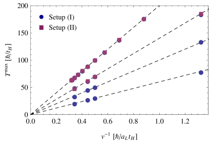
Figure 23 shows the period $T^{\text{max}}$ of the rectangular current oscillation in the finite system as a function of the inverse renormalized Fermi velocity $v^{-1}$ from expression (2). The $T^{\text{max}}$ values are mean values from various $\Delta\epsilon$ for each setup. These values agree perfectly with the dashed lines in Fig. 23 which are given by the equation

$$T^{\text{max}}(V_{\text{H}})=\frac{v(V_{\text{H}}=0)}{v(V_{\text{H}})}T^{\text{max}}(V_{\text{H}}=0).$$ (71)

Thus, the period is fully determined by the time-scale of the non-interacting system $T^{\text{max}}(V_{\text{H}}=0)$ from (77) and the renormalized Fermi velocity $v$ from expression (2).

VI Summary and conclusion

We have presented a method for investigating the non-linear steady-state transport properties of one-dimensional correlated quantum systems. First, we have analyzed finite-size effects and transient currents in a related classical model, the so-called $LC$ line. This exact analysis shows how steady-state currents in the thermodynamic limit can be calculated from transient currents in finite systems. We have found that for currents in quantum systems, in particular the spinless fermion model, finite-size effects can be understood from the behaviour of the $LC$ line.

On the basis of the strong connection between the finite-size behaviour in classical and quantum models we have developed a method to extract a stationary current from simulations of finite-size quantum systems. We only need numerical data $I(t)$ up to a time of the order of $T^{\text{max}}/4$ where $T^{\text{max}}\propto N$ is the period of the approximately rectangular signal $I(t)$ in a quantum system of size $N$. The non-equilibrium dynamics of correlated quantum systems has been calculated using the time-evolving block decimation method (TEBD). We have implemented a multi-threaded version of TEBD with an extremely low overhead (less than 1% for 10 threads) which allows us to simulate the non-equilibrium dynamics up to the time-scale $2T^{\text{max}}$.

We have determined the full $I$–$V$ characteristic of the spinless fermion model with nearest-neighbour hopping $t_{\text{H}}$ and interaction $V_{\text{H}}$ using two different setups to generate currents. In setup (I) the initial state has different particle numbers in its two halves due to an applied potential difference while the system evolves in time with an overall equal on-site potential. In setup (II) we calculate the initial state without a potential difference but turn it on for the real time evolution. For non-interacting fermions ($V_{\text{H}}=0$) our outcomes agree with the analytical solutions and with the results of the one-particle equation of motion method. Additionally, we have checked that our results coincide with the field-theoretical analysis and td-DMRG simulationsBoulat08 for the IRLM.

For interacting fermions we have found that the steady-state current is independent from the setup in the linear regime $|eV|\ll 4t_{\text{H}}$. Moreover, our numerical data agree with the predictions of the Luttinger liquid theory combined with the Bethe Ansatz solution. For larger potentials $V$ the steady-state current depends on the current-generating setup. This difference is well understood for non-interacting systems Branschaedel10 ; Baldea10 but can only be explained qualitatively for our interacting system. With setup (I) we have found that the current increases with $V$ and saturates at a finite value when the potential difference is high enough to separate the initial state in one filled and one empty half. With setup (II) we observe a negative differential conductance that can be understood in terms of the overlap of the elementary excitation bands in the spinless Luttinger liquids in the two halves of the system. Both effects – the plateaus and the negative differential conductance at large potential bias – are due to the finite bandwidth of the system which agrees with the findings in Ref. Baldea10, . However, in our case the interaction renormalizes the effective bandwidth exactly as the Fermi velocity in equation (2) so that the current maxima and the onset of the plateaus depend on the strength of the interaction $V_{\text{H}}$. The change in the typical time-scale $T^{\text{max}}$ also solely depends on the renormalized Fermi velocity.

The methods presented in this work can be applied to other systems, such as models of quantum dots or wires coupled to leads including electronic and also bosonic degrees of freedom. We have already checked the applicability of these methods to the IRLM, the one-dimensional Hubbard model away from half-filling and also two-leg ladder systems. Hence, we believe that they will be very useful to study non-linear transport properties of correlated low-dimensional conductors. Although we have mostly tested our appraoch in the limit of transparent coupling between source and drain, we think that it can also be applied when the hybridization between leads is very small. This issue will be examined in future works.

Appendix A Approximations of the Bessel und Struve functions

The Bessel functions of the first kind and Struve functions have the following approximations which become exact for $x\rightarrow\infty$

$$\mathcal{J}_{0}(x) = \sqrt{\frac{2}{\pi x}}\cos\left(x-\frac{\pi}{4}\right)+\mathcal{O}\left(\frac{1}{x}\right),$$

$$\mathcal{J}_{1}(x) = \sqrt{\frac{2}{\pi x}}\cos\left(x-\frac{3}{4}\pi\right)+\mathcal{O}\left(\frac{1}{x}\right),$$

$$\mathcal{H}_{0}(x) = \sqrt{\frac{2}{\pi x}}\sin\left(x-\frac{\pi}{4}\right)+\mathcal{O}\left(\frac{1}{x}\right),$$

$$\mathcal{H}_{1}(x) = \frac{2}{\pi}-\sqrt{\frac{2}{\pi x}}\cos\left(x-\frac{\pi}{4}\right)+\mathcal{O}\left(\frac{1}{x}\right).$$ (72)

Using these expressions together with equation (44) yields the stationary current value (45) but does not provide an approximate expression for the short-time behaviour of the current, since all time-dependent terms cancel out. Instead, the asymptotic series expansions from Refs. Abramowitz72, and Erdelyi56, and the approximation of $\mathcal{H}_{1}(x)$Aarts03

$$\mathcal{J}_{0}(x) = \frac{(8x-1)\cos(x)+(8x+1)\sin(x)}{8\sqrt{\pi x^{3}}}+\mathcal{O}\left(\frac{1}{x^{\frac{5}{2}}}\right),$$

$$\mathcal{J}_{1}(x) = \frac{(3-8x)\cos(x)+(3+8x)\sin(x)}{8\sqrt{\pi x^{3}}}+\mathcal{O}\left(\frac{1}{x^{\frac{5}{2}}}\right),$$

$$\mathcal{H}_{0}(x) = \frac{8x\sqrt{\pi}(\sin(x)-\cos(x))+16\sqrt{x}-\sqrt{\pi}}{8\pi\sqrt{x^{3}}}$$

$$\quad+~{}\mathcal{O}\left(\frac{1}{x^{\frac{5}{2}}}\right),$$

$$\mathcal{H}_{1}(x) \approx \frac{2}{\pi}+\frac{\left(\frac{16}{\pi}-5\right)\sin{x}}{x}$$ (73)

$$\quad+~{}\frac{\left(12-\frac{36}{\pi}\right)(1-\cos(x))}{x^{2}}-\mathcal{J}_{0}(x)$$

result in the expression (47).

Appendix B Period of the rectangular oscillation in the tight-binding model

The time evolution of the single particle reduced density matrix (14) is given by

$$\mathcal{G}_{ij}(t)=\exp{\left(-\frac{i}{\hbar}\varepsilon_{q}t\right)}\mathcal{G}_{kq}(0)\exp{\left(\frac{i}{\hbar}\varepsilon_{k}t\right)}$$ (74)

in the eigenbasis of a time-constant single particle Hamiltonian $H^{(1)}$. $\Psi_{k,i}$ denotes the $i$-th component of the $k$-th eigenvector of $H^{(1)}$ and $\varepsilon_{k}$ the corresponding eigenvalue. A Fourier transformation gives

$$\tilde{\mathcal{G}}_{kq}(\omega)=\delta\left[\varepsilon_{k}-\varepsilon_{q}-\hbar\omega\right]\mathcal{G}_{kq}(0).$$ (75)

For the tight-binding model with zero on-site potentials one has

$$\Psi_{k,i} = \sqrt{\frac{2}{N+1}}\sin\left(\frac{ki\pi}{N+1}\right),$$

$$\varepsilon_{k} = -2t_{\text{H}}\cos\left(\frac{k\pi}{N+1}\right).$$ (76)

The period of the largest (rectangular) oscillation is then given by

$$T^{\text{max}}=\frac{\pi\hbar}{t_{\text{H}}\sin\left(\frac{\pi}{N+1}\right)}\approx\hbar\cdot\frac{N}{t_{\text{H}}}\quad\text{for}\quad N\gg 1.$$ (77)

Appendix C Current in the infinite one-dimensional tight-binding model

The expectation value of the current for setup (I) and for initial conditions like in Fig. 12 (one completely filled and one completely empty half) is for $N\rightarrow\infty$ given byAntal99 ; Hunyadi04

$$J_{\text{F}}^{k}(t)=\frac{2et_{\text{H}}}{\hbar}\sum_{l=k-\frac{N}{2}}^{\infty}\mathcal{J}_{l}(\omega t)\mathcal{J}_{l+1}(\omega t)$$ (78)

where $k$ denotes the site, $\omega=2t_{\text{H}}/\hbar$ and $\mathcal{J}_{l}(z)$ are the Bessel functions of the first kind. Reformulating the sum and utilizing the Bessel recursion relation

$$\frac{2l}{z}\mathcal{J}_{l}(z)=\mathcal{J}_{l+1}(z)+\mathcal{J}_{l-1}(z)$$ (79)

gives for $z\neq 0$ and $k=N/2$

$$J_{\text{F}}(\omega t)=J_{\text{F}}^{N/2}(\omega t)=\frac{4et_{\text{H}}}{\hbar\omega t}\sum_{l=0}^{\infty}\left[(\mathcal{J}_{2l+1}(\omega t))^{2}\cdot(2l+1)\right].$$ (80)

WithAbramowitz72

$$\sum_{l=0}^{\infty}(4l+2\nu+2)\mathcal{J}_{2l+\nu+1}(z)\mathcal{J}_{2l+\nu+1}(w)$$

$$=\frac{zw}{z^{2}-w^{2}}\left[z\mathcal{J}_{\nu+1}(z)\mathcal{J}_{\nu}(w)-w\mathcal{J}_{\nu}(z)\mathcal{J}_{\nu+1}(w)\right]$$ (81)

for $\text{Re}(\nu)>-1$ and $z\neq w$ the current is given by

$$J_{\text{F}}(t)=\frac{2et_{\text{H}}}{\hbar}\lim_{t^{\prime}\rightarrow t}\frac{\omega t\mathcal{J}_{1}(\omega t)\mathcal{J}_{0}(\omega t^{\prime})-\omega t^{\prime}\mathcal{J}_{0}(\omega t)\mathcal{J}_{1}(\omega t^{\prime})}{(\pi\omega t^{\prime})^{-1}((\omega t)^{2}-(\omega t^{\prime})^{2})}.$$ (82)

Applying l’Hôspital’s rule one gets

$$J_{\text{F}}(t)=\frac{et_{\text{H}}}{\hbar}\omega t\left[(\mathcal{J}_{0}(\omega t))^{2}+(\mathcal{J}_{1}(\omega t))^{2}\right].$$ (83)

References

- (1) K. Schönhammer, J. Phys.: Condens. Matter 14, 12783 (2002).
- (2) T. Giamarchi, Quantum Physics in One Dimension (Clarendon Press, Oxford, 2003).
- (3) K. Schönhammer, in Strong Interactions in Low Dimensions, edited by D. Baeriswyl and L. Degiorgi (Kluwer Academic Publishers, Dordrecht, 2004).
- (4) A. Yacoby, in Strong Interactions in Low Dimensions, edited by D. Baeriswyl and L. Degiorgi (Kluwer Academic Publishers, Dordrecht, 2004).
- (5) X. Zotos and P. Prelovsek, in Strong Interactions in Low Dimensions, edited by D. Baeriswyl and L. Degiorgi (Kluwer Academic Publishers, Dordrecht, 2004).
- (6) A. Kawabata, Rep. Prog. Phys. 70, 219 (2007).
- (7) C.L. Kane and M.P.A. Fisher, Phys. Rev. Lett. 68, 1220 (1992).
- (8) A. Furusaki and N. Nagaosa, Phys. Rev. B 47, 4631 (1993).
- (9) P. Fendley, A.W.W. Ludwig, and H. Saleur, Phys. Rev. B 52, 8934 (1995).
- (10) A. Komnik and H. Saleur, Phys. Rev. Lett. 107, 100601 (2011).
- (11) G. Barak, H. Steinberg, L.N. Pfeiffer, K.W. West, L. Glazman, F. von Oppen, and A. Yacoby, Nature Physics 6, 489 (2010).
- (12) E. Boulat, H. Saleur, and P. Schmitteckert, Phys. Rev. Lett. 101, 140601 (2008).
- (13) F. Heidrich-Meisner, A.E. Feiguin, and E. Dagotto, Phys. Rev. B 79, 235336 (2009).
- (14) S. T. Carr, D. A. Bagrets, and P. Schmitteckert, Phys. Rev. Lett. 107, 206801 (2011).
- (15) U. Schollwöck and S.R. White in Effective models for low-dimensional strongly correlated systems, edited by G.G. Batrouni and D. Poilblanc (AIP, New York, 2006).
- (16) R.M. Noack, S.R. Manmana, S. Wessel, A. and Muramatsu, in Computational Many-Particle Physics, edited by H. Fehske, R. Schneider, and A. Weiße (Springer, Berlin, 2008).
- (17) U. Schollwöck, Annals of Physics 326, 96 (2011).
- (18) G. Vidal, Phys. Rev. Lett. 91, 147902 (2003).
- (19) G. Vidal, Phys. Rev. Lett. 93, 040502 (2004).
- (20) M.A. Cazalilla and J.B. Marston, Phys. Rev. Lett. 88, 256403 (2002).
- (21) H.G. Luo, T. Xiang and X.Q. Wang, Phys. Rev. Lett. 91, 049701 (2003).
- (22) M.A. Cazalilla and J.B. Marston, Phys. Rev. Lett. 91, 049702 (2003).
- (23) P. Schmitteckert, Phys. Rev. B 70, 121302 (2004).
- (24) K.A. Al-Hassanieh, A.E. Feiguin, J.A. Riera, C.A. Büsser, and E. Dagotto, Phys. Rev. B 73, 195304 (2006).
- (25) S. Kirino, T. Fujii, J. Zhao, and K. Ueda, J. Phys. Soc. Japan 77, 084704 (2008).
- (26) F. Heidrich-Meisner, G.B. Martins, K.A. Al-Hassanieh, A.E. Feiguin, G. Chiappe, E.V. Anda, and E. Dagotto, Eur. J. Phys. B 67, 527 (2009).
- (27) S. Kirino and K. Ueda, J. Phys. Soc. Japan 79, 093710 (2010).
- (28) F. Heidrich-Meisner, I. González, K.A. Al-Hassanieh, A.E. Feiguin, M.J. Rozenberg, and E. Dagotto, Phys. Rev. B 82, 205110 (2010).
- (29) M. Žnidarič, Phys. Rev. Lett. 106, 220601 (2011).
- (30) S. Jesenko and M. Žnidarič, Phys. Rev. B 84, 174438 (2011).
- (31) A.J. Daley, C. Kollath, U. Schollwöck, and G. Vidal, J. Stat. Mech. P04005 (2004).
- (32) E. Jeckelmann, in Computational Many-Particle Physics, edited by H. Fehske, R. Schneider, and A. Weiße (Springer, Berlin, 2008).
- (33) G. Hager, E. Jeckelmann, H. Fehske, and G. Wellein, Journal of Computational Physics 194, 795 (2004).
- (34) P. Schmitteckert and G. Schneider in High Performance Computing in Science and Engineering ’06, edited by W.E. Nagel, W. Jäger, and M. Resch (Springer, Berlin, 2007).
- (35) A. Branschädel, G. Schneider, and P. Schmitteckert, Ann. Phys. (Berlin) 522, 657 (2010).
- (36) I. Bâldea and H. Köppel, Phys. Rev. B 81, 193401 (2010).
- (37) E. Perfetto, G. Stefanucci, and M. Cini, Phys. Rev. Lett. 105, 156802 (2010).
- (38) N. Hatano and M. Suzuki, in Quantum Annealing and Other Optimization Methods, edited by A. Das and B.K. Chakrabarti (Springer, Berlin, 2005).
- (39) D. Gobert, C. Kollath, U. Schollwöck, and G. Schütz, Phys. Rev. E 71, 036102 (2005).
- (40) R. Hirota and K. Suzuki, Proc. IEEE 61, 1483 (1973).
- (41) M. Toda, Physics Reports 18, 1 (1975).
- (42) A.C. Singer and A.V. Oppenheim, International Journal of Bifurcation and Chaos 9, 571 (1999).
- (43) G.L. Ingold and Y.V. Nazarov, in Single Charge Tunnelling, edited by H. Grabert and M.H. Devoret (Plenum Press, New York, 1992); Preprint arXiv:cond-mat/0508728 .
- (44) A. Abramowitz and I.A. Stegun, Handbook of Mathematical Functions (Dover Publications, New York, 1972).
- (45) R.M. Aarts and A.J.E.M. Janssen, J. Acoust. Soc. Am. 113, 2635 (2003).
- (46) N. S. Wingreen, A.-P. Jauho, and Y. Meir, Phys. Rev. B 48, 8487 (1993).
- (47) T. Antal, Z. Rácz, A. Rákos, and G.M. Schütz, Phys. Rev. E 59, 4912 (1999).
- (48) V. Hunyadi, Z. Rácz, and L. Sasvári, Phys. Rev. E 69, 066103 (2004).
- (49) S. Langer, F. Heidrich-Meisner, J. Gemmer, I.P. McCulloch, and U. Schollwöck, Phys. Rev. B 79, 214409 (2009).
- (50) A. Kawabata, J. Phys. Soc. Japan 65, 30 (1996).
- (51) I. Safi and H.J. Schulz, Phys. Rev. B 52, 17040 (1995).
- (52) D.L. Maslov and M. Stone, Phys. Rev. B 52, 5539 (1995).
- (53) V.V. Ponomarenko, Phys. Rev. B 52, 8666 (1995).
- (54) K. Janzen, V. Meden, and K. Schönhammer, Phys. Rev. B 74, 085301 (2006).
- (55) A. Erdélyi, Asymptotic Expansions (Dover Publications, New York, 1956).