Processor Allocation for Optimistic Parallelization of Irregular Programs111The original publication is available at www.springerlink.com [24]
Abstract
Optimistic parallelization is a promising approach for the parallelization of irregular algorithms: potentially interfering tasks are launched dynamically, and the runtime system detects conflicts between concurrent activities, aborting and rolling back conflicting tasks. However, parallelism in irregular algorithms is very complex. In a regular algorithm like dense matrix multiplication, the amount of parallelism can usually be expressed as a function of the problem size, so it is reasonably straightforward to determine how many processors should be allocated to execute a regular algorithm of a certain size (this is called the processor allocation problem). In contrast, parallelism in irregular algorithms can be a function of input parameters, and the amount of parallelism can vary dramatically during the execution of the irregular algorithm. Therefore, the processor allocation problem for irregular algorithms is very difficult.
In this paper, we describe the first systematic strategy for addressing this problem. Our approach is based on a construct called the conflict graph, which (i) provides insight into the amount of parallelism that can be extracted from an irregular algorithm, and (ii) can be used to address the processor allocation problem for irregular algorithms. We show that this problem is related to a generalization of the unfriendly seating problem and, by extending Turán’s theorem, we obtain a worst-case class of problems for optimistic parallelization, which we use to derive a lower bound on the exploitable parallelism. Finally, using some theoretically derived properties and some experimental facts, we design a quick and stable control strategy for solving the processor allocation problem heuristically.
Keywords: Irregular algorithms, Optimistic parallelization, Automatic parallelization, Amorphous data-parallelism, Processor allocation, Unfriendly seating, Turán’s theorem.
1 Introduction
The advent of on-chip multiprocessors has made parallel programming a mainstream concern. Unfortunately writing correct and efficient parallel programs is a challenging task for the average programmer. Hence, in recent years, many projects [14, 10, 3, 20] have tried to automate parallel programming for some classes of algorithms. Most of them focus on regular algorithms such as Fourier transforms [9, 19] and dense linear algebra routines [4]. Automation is more difficult when the algorithms are irregular and use pointer-based data structures such as graphs and sets. One promising approach is based on the concept of amorphous data parallelism [17]. Algorithms are formulated as iterative computations on work-sets, and each iteration is identified as a quantum of work (task) that can potentially be executed in parallel with other iterations. The Galois project [18] has shown that algorithms formulated in this way can be parallelized automatically using optimistic parallelization): iterations are executed speculatively in parallel and, when an iteration conflicts with concurrently executing iterations, it is rolled-back. Algorithms that have been successfully parallelized in this manner include Survey propagation [5], Boruvka’s algorithm [6], Delauney triangulation and refinement [12], and Agglomerative clustering [21].
In a regular algorithm like dense matrix multiplication, the amount of parallelism can usually be expressed as a function of the problem size, so it is reasonably straightforward to determine how many processors should be allocated to execute a regular algorithm of a certain size (this is called the processor allocation problem). In contrast, parallelism in irregular algorithms can be a function of input parameters, and the amount of parallelism can vary dramatically during the execution of the irregular algorithm [16]. Therefore, the processor allocation problem for irregular algorithms is very difficult. Optimistic parallelization complicates this problem even more: if there are too many processors and too little parallel work, not only might some processors be idle but speculative conflicts may actually retard the progress of even those processors that have useful work to do, increasing both program execution time and power consumption. This paper222A brief announcement of this work has been presented at SPAA’11 [23]presents the first systematic approach to addressing the processor allocation problem for irregular algorithms under optimistic parallelization, and it makes the following contributions.
-
•
We develop a simple graph-theoretic model for optimistic parallelization and use it to formulate processor allocation as an optimization problem that balances parallelism exploitation with minimizing speculative conflicts (Section 2).
- •
-
•
Using these ideas, we develop an adaptive controller that dynamically solves the processor allocation problem for amorphous data-parallel programs, providing rapid response to changes in the amount of amorphous data-parallelism (Section 4).
2 Modeling Optimistic Parallelization
A typical example of an algorithm that exhibits amorphous data-parallelism is Dalauney mesh refinement, summarized as follows. A triangulation of some planar region is given, containing some “bad” triangles (according to some quality criterion). To remove them, each bad triangle is selected (in any arbitrary order), and this triangle, together with triangles that lie in its cavity, are replaced with new triangles. The retriangulation can produce new bad triangles, but this process can be proved to halt after a finite number of steps. Two bad triangles can be processed in parallel, given that their cavities do not overlap.
There are also algorithms, which exhibit amorphous data-parallelism, for which the order of execution of the parallel tasks cannot be arbitrary, but must satisfy some constraints (e.g., in discrete event simulations the events must commit chronologically). We will not treat this class of problems in this work, but we will focus only on unordered algorithms [16]. A different context in which there is no roll-back and tasks do not conflict, but obey some precedence relations, is treated in [1].
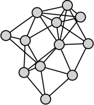
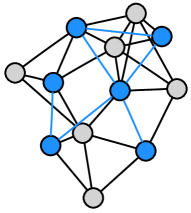
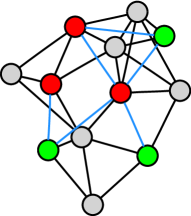
Optimistic parallelization deals with amorphous data-parallelism by maintaining a work-set of the tasks to be executed. At each temporal step some tasks are selected and speculatively launched in parallel. If, at runtime, two processes modify the same data a conflict is detected and one of the two has to abort and roll-back its execution. Neglecting the details of the various amorphous data-parallel algorithms, we can model their common behavior at a higher level with a simple graph-theoretic model: we can think a scheduler as working on a dynamic graph , where the nodes represent computations we want to do, but we have no initial knowledge of the edges, which represent conflicts between computations (see Fig. 1). At time step the system picks uniformly at random nodes (the active nodes) and tries to process them concurrently. When it processes a node it figures out if it has some connections with other executed nodes and, if a neighbor node happens to have been processed before it, aborts, otherwise the node is considered processed, is removed from the graph and some operations may be performed in the neighborhood, such as adding new nodes with edges or altering the neighbors. The time taken to process conflicting and non-conflicting nodes is assumed to be the same, as it happens, e.g., for Dalauney mesh refinement.
 |
 |
 |
||
| (i) | (ii) | (iii) |
2.1 Control Optimization Goal
When we run an optimistic parallelization we have two contrasting goals: we both want to maximize the work done, achieving high parallelism, but at the same time we want to minimize the conflicts, hence obtaining a good use of the processors time. (Furthermore, for some algorithms the roll-back work can be quite resource-consuming.) These two goals are not compatible, in fact if we naïvely try to minimize the total execution time the system is forced to use always all the available processors, whereas if we try to minimize the time wasted from aborted processes the system uses only one processor. Therefore in the following we choose a trade-off goal and cast it in our graph-theoretic model.
Let be a computations/conflicts (CC) graph with nodes. When a scheduler chooses, uniformly at random, nodes to be run, the ordered set by which they commit can be modeled as a random permutation: if then commits before (if there is a conflict between and then commits and aborts, if aborted due to conflicts with previous processes can commit, if not conflicting with other committed processes). Let be the number of aborted processes due to conflicts and the ratio of conflicting processors observed at time (i.e. ). We define the conflict ratio to be the expected that we obtain when the system is run with processors:
| (1) |
where the expectation is computed uniformly over the possible prefixes of length of the nodes permutations. The control problem we want to solve is the following: given and for , choose such that , where is a suitable parameter.
Remark 1.
If we want to dynamically control the number of processors, must be chosen different from zero, otherwise the system converges to use only one processor, thus not being able to identify available parallelism. A value of is often reasonable, together with the constraint .
3 Exploiting Parallelism
In this section we study how much parallelism can be extracted from a given CC graph and how its sparsity can affect the conflict ratio. To this purpose we obtain a worst case class of graphs and use it to analytically derive a lower bound for the exploitable parallelism (i.e., an upper bound for the conflict ratio). We make extensive use of finite differences (i.e., discrete derivatives), which are defined recursively as follows. Let be a real function defined on the integers, then the -th (forward) finite difference of is
| (2) |
(In the following we will omit ’s superscript when equal to one, i.e., .)
First, we obtain two basic properties of , which are given by the following propositions.
Proposition 1.
The conflict ratio function is non-decreasing in .
To prove Prop. 1 we first need a lemma:
Lemma 1.
Let . Then is a non-decreasing convex function, i.e. and .
Proof.
Let be the expected number of conflicting nodes running nodes concurrently, the first of which are and the last are chosen uniformly at random among the remaining ones. By definition, we have
| (3) |
In particular,
| (4) |
which brings
| (5) |
with , hence proving the monotonicity of . Consider now
| (6) |
If the -th node does not add any edge, then we have
| (7) |
but since it may add some edges the probability of conflicting the second time is in general larger and thus . ∎∎
Prop. 1.
Since , its finite difference can be written as
| (8) |
Because of Lemma 1 and being we have
| (9) |
which finally brings
| (10) |
∎∎
Proposition 2.
Let be a CC graph, with nodes and average degree , then the initial derivative of depends only on and as
| (11) |
Proof.
Since
| (12) |
we just need to obtain . Let be defined as in the proof on Lemma 1 and a node chosen uniformly at random. Then
| (13) |
∎∎
A measure of the available parallelism for a given CC graph has been identified in [15] considering, at each temporal step, a maximal independent set of the CC graph. The expected size of a maximal independent set gives a reasonable and computable estimate of the available parallelism. However, this is not enough to predict the actual amount of parallelism that a scheduler can exploit while keeping a low conflict ratio, as shown in the following example.
Example 1.
Let where is the complete graph of size and a disconnected graph of size (i.e. is made up of a clique of size and disconnected nodes). For this graph every maximal independent set is maximum too and has size , but if we choose nodes uniformly at random and then compute the conflicts we obtain that, on average, there are only 2 independent nodes.
A more realistic estimate of the performance of a scheduler can be obtained by analyzing the CC graph sparsity. The average degree of the CC graph is linked to the expected size of a maximal independent set of the graph by the following well known theorem (in the variant shown in [2] or [22]):
Theorem 1.
(Turán, strong formulation). Let be a graph, and let be the average degree of . Then the expected size of a maximal independent set, obtained choosing greedily the nodes from a random permutation, is at least .
Remark 2.
The previous bound is existentially tight: let be the graph made up of cliques of size , then the average degree is and the size of every maximal (and maximum) independent set is exactly . Furthermore, every other graph with the same number of nodes and edges has a bigger average maximal independent set.
The study of the expected size of a maximal independent set in a given graph is also known as the unfriendly seating problem [7, 8] and is particularly relevant in statistical physics, where it is usually studied on mesh-like graphs [11]. The properties of the graph has suggested us the formulation of an extension of the Turán’s theorem. We prove that the graphs provide a worst case (for a given degree ) for the generalization of this problem obtained by focusing on maximal independent set of induced subgraphs. This allows, when given a target conflict ratio , the computation of a lower bound for the parallelism a scheduler can exploit.
Theorem 2.
Let be a graph with same nodes number and degree of and let be the expected size of a maximal independent set of the subgraph induced by a uniformly random choice of nodes in , then
| (14) |
To prove it we first need the following lemma.
Lemma 2.
The function is convex for .
Proof.
We prove by induction on that, for ,
| (15) |
Base case
Let . The properties above are easily verified.
Induction
Since , we obtain
| (16) |
which is non-positive by inductive hypotheses. Similarly,
| (17) |
is non-negative. ∎∎
Thm. 2.
Consider a random permutation of the nodes of a generic graph that has the same number of nodes and edges of . We assume the prefix of length of (i.e. ) forms the active nodes and focus on the following independent set in the subgraph induced: a node is in if and only if it is in the first positions of and it has no neighbors preceding it. Let be the expected size of averaged over all possible ’s (chosen uniformly):
| (18) |
Since for construction whereas , we just need to prove that . Given a generic node of degree and a random permutation , its probability to be in is
| (19) |
By the linearity of the expectation we can write as
| (20) | ||||
| (21) |
To prove that is thus enough showing that
| (22) |
which can be done applying Jensen’s inequality [13], since in Lemma 2 we have proved the convexity of . ∎∎
Corollary 1.
The worst case for a scheduler among the graphs with the same number of nodes and edges is obtained for the graph (for which we can analytically approximate the performance, as shown in §3.1).
Proof.
Since
| (23) |
the thesis follows. ∎∎
3.1 Analysis of the Worst-Case Performance
Theorem 3.
Let be the average degree of with (for simplicity we assume ). The conflict ratio is bounded from above as
| (24) |
Proof.
Let be the number of connected components in . Because of Thm. 2 and Cor. 1 it suffices to show that
| (25) |
The probability for a connected component of not to be accessed when nodes are chosen is given by the following hypergeometric
| (26) |
Let be a random variable that is 1 when component is hit and 0 otherwise. We have that and, by the linearity of the expectation, the average number of components accessed is
| (27) |
∎∎
Corollary 2.
When and increase the bound is well approximated by
| (28) |
Proof.
Stirling approximation for the binomial, followed by low order terms deletion in the resulting formula. ∎∎
Corollary 3.
If we set we obtain
| (29) |
4 Controlling Processors Allocation
In this section we will design an efficient control heuristic that dynamically chooses the number of processes to be run by a scheduler, in order to obtain high parallelism while keeping the conflict ratio low. In the following we suppose that the properties of are varying slowly compared to the convergence of toward under the algorithm we will develop (see §4.1), so we can consider and and thus our goal is making converge to .
Since the conflict ratio is a non-decreasing function of the number of launched tasks (Prop. 1) we could find by bisection simply noticing that
| (30) |
The control we propose is slightly more complex and is based on recurrence relations, i.e., we compute as a function of the target conflict ratio and of the parameters which characterize the system at the previous timestep:
| (31) |
The initial value for a recurrence can be chosen to be 2 but, if we have an estimate of the CC graph average degree , we can choose a smarter value: in fact applying Cor. 3 we are sure that using, e.g., processors we will have at most a conflict ratio of .
Our control heuristic (Algorithm 1) is a hybridization of two simple recurrences. The first recurrence is quite natural and increases based on the distance between and :
| (32) |
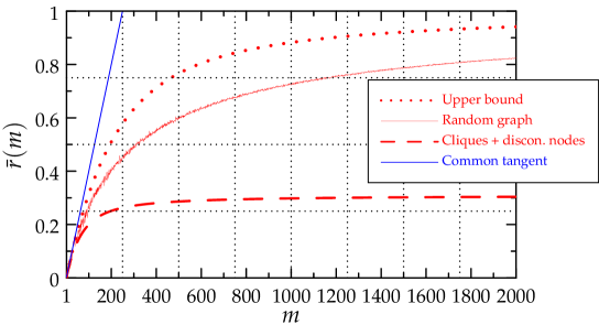
The second recurrence exploits some experimental facts. In Fig. 2 we have plotted the conflict ratio functions for three CC graphs with the same size and average degree (note that initial derivative is the same for all the graphs, in accordance with Prop. 2). We see that conflict ratios which reach a high value () are initially well approximated by a straight line (for such that ), whereas functions that deviates from this behavior do not raise too much. This suggests us to assume an initial linearity in controlling , as done by the following recurrence:
| (33) |
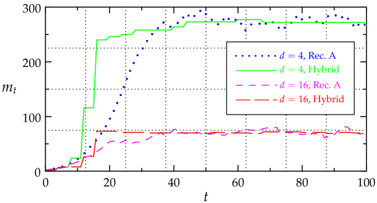
The two recurrences can be roughly compared as follows (see Fig. 3): Recurrence A has a slower convergence than Recurrence B, but it is less susceptible to noise (the variance that makes realizations different from ). This is the reason for which we chose to merge them in an hybrid algorithm: initially, when the difference between and is big, we use Recurrence B to exploit its quick convergence and then Recurrence A is adopted, for a finer tuning of the control.
4.1 Experimental Evaluation
In the practical implementation of the control algorithm we have made the following optimizations:
-
•
Since can have a big variance, especially when is small, we decided to apply the changes to every steps, using the averaged values obtained in these intervals, to smooth the oscillations.
-
•
To further reduce the oscillations we apply a change only if the observed is sufficiently different from (e.g. more than ), thus avoiding small variations in the steady state, which interfere with locality exploitation because of the data moving from one processor to another.
-
•
Another problem that must be considered is that for small values of the variance is much bigger, so it is better to tune separately this case using different parameters (this optimization is not shown in the pseudo-code).
To validate our controller we have run the following simulation: a random CC graph of fixed average degree is taken and the controller runs on it, starting with . We are interested in seeing how many temporal steps it takes to converge to . As can be seen in [15] the parallelism profile of many practical applications can vary quite abruptly, e.g., Delauney mesh refinement can go from no parallelism to one thousand possible parallel tasks in just 30 temporal steps. Therefore, an algorithm that wants to efficiently control the processors allocations for these problems must adapt very quickly to changes in the available parallelism. Our controller, that uses the very fast Recurrence B in the initial phase, proves to do a fast enough job: as shown in Fig. 3 in about 15 steps the controller converges close to the desired value.
5 Conclusions and Future Work
Automatic parallelization of irregular algorithms is a rich and complex subject and will offer many difficult challenges to researchers in the next future. In this paper we have focused on the processor allocation problem for unordered data-amorphous algorithms; it would be extremely valuable to obtain similar results for the more general and difficult case of ordered algorithms (e.g., discrete event simulation), in particular it is very hard to obtain good estimates of the available parallelism for such algorithms, given the complex dependencies arising between the concurrent tasks. Another aspect which needs investigation, especially in the ordered context, is whether some statical properties of the behavior of irregular algorithms can be modeled, extracted and exploited to build better controllers, able to dynamically adapt to the different execution phases.
As for a real-world implementation, the proposed control heuristic is now being integrated in the Galois system and it will be evaluated on more realistic workloads.
Acknowledgments
We express our gratitude to Gianfranco Bilardi for the valuable feedback on recurrence-based controllers and to all the Galois project members for the useful discussions on optimistic parallelization modeling.
References
- [1] Agrawal, K., Leiserson, C.E., He, Y., Hsu, W.J.: Adaptive work-stealing with parallelism feedback. ACM Trans. Comput. Syst. 26(3), 7:1–7:32 (Sep 2008), http://doi.acm.org/10.1145/1394441.1394443
- [2] Alon, N., Spencer, J.: The probabilistic method. Wiley-Interscience (2000)
- [3] An, P., Jula, A., Rus, S., Saunders, S., Smith, T.G., Tanase, G., Thomas, N., Amato, N.M., Rauchwerger, L.: Stapl: An adaptive, generic parallel C++ library. In: Dietz, H.G. (ed.) LCPC. Lecture Notes in Computer Science, vol. 2624, pp. 193–208. Springer (2001)
- [4] Blackford, L.S., Choi, J., Cleary, A., D’Azevedo, E., Demmel, J., Dhillon, I., Dongarra, J., Hammarling, S., Henry, G., Petitet, A., Stanley, K., Walker, D., Whaley, R.C.: ScaLAPACK Users’ Guide. Society for Industrial and Applied Mathematics, Philadelphia, PA (1997)
- [5] Braunstein, A., Mézard, M., Zecchina, R.: Survey propagation: An algorithm for satisfiability. Random Struct. Algorithms 27(2), 201–226 (2005)
- [6] Eppstein, D.: Spanning trees and spanners. In: Sack, J., Urrutia, J. (eds.) Handbook of Computational Geometry, pp. 425–461. Elsevier (2000)
- [7] Freedman, D., Shepp, L.: Problem 62-3, an unfriendly seating arrangement. SIAM Review 4(2), p. 150 (1962), http://www.jstor.org/stable/2028372
- [8] Friedman, H.D., Rothman, D., MacKenzie, J.K.: Problem 62-3. SIAM Review 6(2), pp. 180–182 (1964), http://www.jstor.org/stable/2028090
- [9] Frigo, M., Johnson, S.G.: The design and implementation of FFTW3. Proceedings of the IEEE 93(2), 216–231 (2005), special issue on “Program Generation, Optimization, and Platform Adaptation”
- [10] Frigo, M., Leiserson, C.E., Randall, K.H.: The implementation of the Cilk-5 multithreaded language. In: PLDI. pp. 212–223 (1998)
- [11] Georgiou, K., Kranakis, E., Krizanc, D.: Random maximal independent sets and the unfriendly theater seating arrangement problem. Discrete Mathematics 309(16), 5120 – 5129 (2009), http://www.sciencedirect.com/science/article/B6V00-4W55T4X-2/2/72d38a668c737e68edf497512e606e12
- [12] Guibas, L.J., Knuth, D.E., Sharir, M.: Randomized incremental construction of delaunay and voronoi diagrams. Algorithmica 7(4), 381–413 (1992)
- [13] Jensen, J.: Sur les fonctions convexes et les inégalités entre les valeurs moyennes. Acta Mathematica 30(1), 175–193 (1906)
- [14] Kalé, L.V., Krishnan, S.: Charm++: A portable concurrent object oriented system based on C++. In: OOPSLA. pp. 91–108 (1993)
- [15] Kulkarni, M., Burtscher, M., Cascaval, C., Pingali, K.: Lonestar: A suite of parallel irregular programs. In: ISPASS. pp. 65–76. IEEE (2009)
- [16] Kulkarni, M., Burtscher, M., Inkulu, R., Pingali, K., Cascaval, C.: How much parallelism is there in irregular applications? In: Reed, D.A., Sarkar, V. (eds.) PPOPP. pp. 3–14. ACM (2009)
- [17] Méndez-Lojo, M., Nguyen, D., Prountzos, D., Sui, X., Hassaan, M.A., Kulkarni, M., Burtscher, M., Pingali, K.: Structure-driven optimizations for amorphous data-parallel programs. In: Govindarajan, R., Padua, D.A., Hall, M.W. (eds.) PPOPP. pp. 3–14. ACM (2010)
- [18] Pingali, K., Nguyen, D., Kulkarni, M., Burtscher, M., Hassaan, M.A., Kaleem, R., Lee, T.H., Lenharth, A., Manevich, R., Méndez-Lojo, M., Prountzos, D., Sui, X.: The tao of parallelism in algorithms. In: Proceedings of the 32nd ACM SIGPLAN conference on Programming language design and implementation. pp. 12–25. PLDI ’11, ACM, New York, NY, USA (2011), http://doi.acm.org/10.1145/1993498.1993501
- [19] Püschel, M., Moura, J., Johnson, J., Padua, D., Veloso, M., Singer, B., Xiong, J., Franchetti, F., Gacic, A., Voronenko, Y., Chen, K., Johnson, R., Rizzolo, N.: Spiral: Code generation for dsp transforms. Proceedings of the IEEE 93(2), 232–275 (Feb 2005)
- [20] Reinders, J.: Intel threading building blocks. O’Reilly & Associates, Inc., Sebastopol, CA, USA (2007)
- [21] Tan, P.N., Steinbach, M., Kumar, V.: Introduction to Data Mining. Addison-Wesley (2005)
- [22] Tao, T.: Additive combinatorics. Cambridge University Press (2006)
- [23] Versaci, F., Pingali, K.: Brief announcement: processor allocation for optimistic parallelization of irregular programs. In: Proceedings of the 23rd ACM symposium on Parallelism in algorithms and architectures. pp. 261–262. SPAA ’11, ACM, New York, NY, USA (2011), http://doi.acm.org/10.1145/1989493.1989533
- [24] Versaci, F., Pingali, K.: Processor allocation for optimistic parallelization of irregular programs. In: Murgante, B., Gervasi, O., Misra, S., Nedjah, N., Rocha, A., Taniar, D., Apduhan, B. (eds.) Computational Science and Its Applications – ICCSA 2012, Lecture Notes in Computer Science, vol. 7333, pp. 1–14. Springer Berlin / Heidelberg (2012), http://dx.doi.org/10.1007/978-3-642-31125-3_1