Transit Monitoring in the South (TraMoS) project: Discarding Transit Timing Variations in WASP-5b
Abstract
We report nine new transit epochs of the extrasolar planet WASP-5b (catalog ), observed in the Bessell I band with SOAR at the Cerro Pachon Observatory and with the SMARTS 1-m Telescope at CTIO111Based on observations made with the SMARTS 1-m telescope at CTIO and the SOAR Telescope at Cerro Pachon Observatory under programmes ID CNTAC-08B-046,-09A-089 and -09B-050. , between August 2008 and October 2009. The new transits have been combined with all previously published transit data for this planet to provide a new Transit Timing Variations (TTVs) analysis of its orbit. We find no evidence of TTVs RMS variations larger than 1 min over a 3 year time span. This result discards the presence of planets more massive than about , and around the 1:2, 5:3 and 2:1 orbital resonances. These new detection limits exceed by times the limits imposed by current radial velocity observations in the Mean Motion Resonances of this system. Our search for the variation of other parameters, such as orbital inclination and transit depth also yields negative results over the total time span of the transit observations. This result supports formation theories that predict a paucity of planetary companions to Hot Jupiters.
1 Introduction
Once the method of Transit Timing Variations (TTVs) was theoretical proposed as of great potential to detect additional exoplanets in transiting systems (Miralda-Escudé 2002; Agol et al. 2005; Holman & Murray 2005), and even exomoons (Sartoretti & Schneider 1999; Kipping 2009), several observational groups have started to monitor the majority of the known transiting planets. This monitoring aims at detecting changes in the predicted mid-time of the transits to infer the presence of additional planets in the system not detected previously by e.g. radial velocities. Those data have also been used to detect variations in other transit parameters (e.g. transit depth and duration), that can be attributed to perturbations produced by unseen companions (Miralda-Escudé 2002).
In addition to having the potential of finding planets in the Earth-like or smaller mass regime, the detection (or non-detection) of companions of transiting Hot Jupiters through TTVs also can improve constraints on planet formation models (e.g. Triaud et al. 2010; Naoz et al. 2011; Miguel et al. 2011, and references therein) and help discriminate between the different mechanisms proposed. In this way, TTVs become a powerful tool for the detection and study of multi-planet system architectures (Latham et al. 2011; Ford et al. 2011).
The first unquestionable evidence of TTVs was announced by Holman et al. (2010) in the double Saturn-like transiting planetary system Kepler-9 (catalog ), where the central times of transit vary with amplitudes of 4 and 39 minutes in timescales of about 19 and 40 days, respectively. Another extraordinary confirmation of the TTVs effect came with the discovery of Kepler-11 (Lissauer et al. 2011), a system with six transiting planets which shows TTVs of amplitudes as large as tens of minutes produced by the gravitational perturbations between the planets. An additional remarkable result of this later work has been the use of dynamical orbital fits to determine directly the masses of the transiting planets, dismissing the need of radial velocities.
In 2008, the WASP-South survey reported their second detection of an exoplanet, WASP-5b (catalog ), transiting a relatively bright star () in the Southern Hemisphere (Anderson et al. 2008, hereafter A08). This discovery paper, based on WASP photometry and two additional transit epochs plus radial velocities measurements, announced a Hot-Jupiter planet with a mass of and a density of , orbiting a G4V star with a period of days.
Gillon et al. (2009) did a reanalysis of the A08 data to produce the first timing study of WASP-5b (catalog ) and arrived to the conclusion of potential period variations, based on a -minute shift in the timing residuals of the most precise points.
Southworth et al. (2009), hereafter S09, observed two new transits, for which they achieved very high photometric precision by defocusing the images at the 1.54-m Danish Telescope at La Silla Observatory, but at the expense of producing only 3-minute cadence. They refined the linear ephemeris of the system and concluded the high deviation of the timing residuals with respect to that straight line () found by Gillon et al. (2009) was based on the divergence of only one point out of six. Smith et al. (2009) searched for signatures of additional planets in the residuals of WASP light curves after removing the transits of WASP-5b (catalog ), and found no evidence of a transiting companion down to Saturn-size planets within periods of up to 20 days.
Other recent works have determined and refined several physical parameters of the system. For example, Triaud et al. (2010) determined the angle between the orbital plane of WASP-5b (catalog ) and the spin axis direction of its host star to be consistent with zero (). This conclusion has been confirmed by the reanalysis of Fukui et al. (2011), hereafter F11, who obtain .
F11 additionally searched for TTVs of WASP-5b (catalog ) using seven new transit epochs, combined with all previously available observations. They find a of about 68 seconds in their timing residuals despite of having an average of 41 seconds uncertainty per epoch, and proposed that such a large deviation from a linear fit ( for 9 degrees of freedom) can be explained by an orbital perturber. Using dynamical simulations F11 constrained the masses of this hypothetical perturber to in the 1:2 and 2:1 mean motion resonances (MMRs) and set a mass of for a potential Trojan body.
Dragomir et al. (2011), hereafter D11, reported two new transits of WASP-5b with data of the 1-m telescope at Cerro Tololo Inter-American Observatory.
In this work we present nine additional transits of WASP-5b (catalog ), observed between August 2008 and October 2009, and perform a new homogeneous timing analysis of all available epochs to further confirm or rule out the TTV signals previously proposed for this system.
2 Observations and data reduction
In 2008 we started the Transit Monitoring in the South Project, which is a monitoring campaign of transiting planets observable from the Southern Hemisphere (Hoyer et al. 2011), following the approach of using high-cadence observations and the same instruments and setups to try to minimize systematics and reduce uncertainties in the mid-transit times, as well as other transit parameters. For the TraMoS project we have already observed more than 60 transits of over 20 exoplanets.
As part of TraMoS we observed a total of nine transits of WASP-5b (catalog ), between August 2008 and October 2009222In the remaining of the text we refer to each individual transit by the UT date of mid-time of the transit, using the following notation YYYY-MM-DD, with the Y4KCam on the SMARTS 1-m Telecope at Cerro Tololo Inter-American Observatory (CTIO) and with the SOAR Optical Imager (SOI) at the 4.2-meter Southern Astrophysical Research (SOAR) telescope in Cerro Pachón.
Y4KCam is a CCD camera with a Field of View (FoV) of squared arcminutes and a pixel scale of 0.289 arcsec pixel-1. The standard readout time of the camera is sec, which we reduce to sec by binning 2x2. The SOI detector is composed of two E2V mosaics of pixels with a scale of 0.077 arcsec pixel-1, giving a FoV of squared arcminutes. The instrument has a sec standard readout, which becomes only sec after binning 2x2.
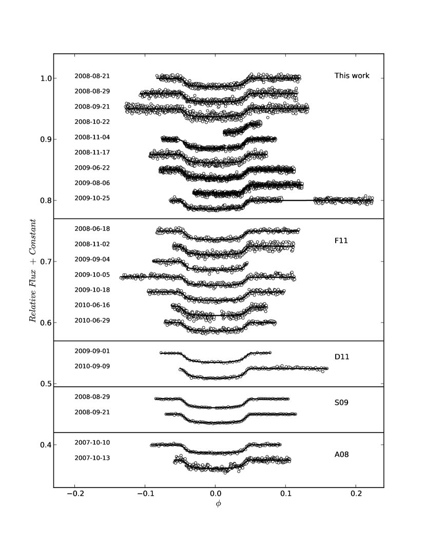
All nine transits were observed using a Bessell I filter ( and FWHM=) to reduce limb darkening effects in our light curves. Six of the transits were fully covered in phase. A fraction of the ingress of the 2008-11-03 transit was not observed because a telescope system crash as illustrated in Figure 1. Nevertheless, this transit was treated as a complete transit. Two other transits, 2009-08-05 and 2009-10-21, were only partially covered with data between phases and , respectively. Two of our transits, 2008-08-29 and 2008-09-21, coincide with the transit epochs published by S09. The observing log is summarized in Table 1.
The initial trimming, bias and flatfield corrections of all the collected data were performed using custom-made pipelines specifically developed for each instrument. The times at the start of the exposure are recorded in the image headers, in particular we used the value of the Modified Julian Day (JD-2400000.5) field. In the SMARTS telescope, the time stamp recorded in the header of each frame is generated by a IRIG-B GPS time synchronization protocol connected to the computers that control the instrument. The SOAR telescope data use the time values provided by a time service connected to the instrument. We confirmed that these values have second precision. The time value assigned to each frame corresponds to the Julian Day at the start of the exposure plus of the integration time of each image (see section 4 for details).
WASP-5 (catalog ) is located in a relative empty field, where both the target and several well suited comparison stars appear well isolated in our images. Therefore, we extracted the flux from the target and comparison stars via standard aperture photometry, and using our own python-based code. We used a range of stellar apertures between 8 and 12 pixels, and sky rings which extended between 25 and 35 pixels in radius.
For each sky-aperture combination, we generated differential light curves between the target and each comparison star to 1) optimize the apertures and 2) select the best comparison stars. The criterium used in both cases was RMS minimization for the out-of-transit and in-transit data (excluding the ingress and egress portions of the light curves). The final light curves were generated computing the ratio between target’s flux and the best 2 to 5 comparison stars.
Finally, some systematics remaining after this step were removed by means of linear or quadratic regression fits to the out-of-transit light curve points using X-Y pixel position, time and/or airmass as free parameters. The final light curves present average photometric dispersions of the order of - .
3 Light Curve Modeling
3.1 Algorithm Comparison
We performed a comparison between algorithms that use different statistical uncertainty estimation techniques to the transit’s parameters, in order to test potential systematics between them. There are different approaches to do that statistical error estimation analysis; for example, JKTEBOP333http://www.astro.keele.ac.uk/ jkt/codes/jktebop.html (Southworth et al. 2004a, b) uses the Levenberg-Marquardt Monte Carlo (LMMC) technique to compute errors (see e.g. Southworth 2010; Hoyer et al. 2011), while several other studies have started to implement Monte Carlo Markov Chains (MCMC) techniques (e.g. Adams et al. 2010; Fulton et al. 2011).
In Hoyer et al. (2011) we proposed that the results of both, the LMMC and MCMC algorithms are equivalent if the parameter space lacks of local minima, where LMMC minimization can be trapped. Here we further test that proposal by comparing the results of both algorithms on the WASP-5b (catalog ) data used for this study. We compare the results of fitting a light curve of WASP-5b with JKTEBOP and the Transit Analysis Package444http://ifa.hawaii.edu/users/zgazak/ifA/TAP.html (TAP; Gazak et al. 2011), which implements the MCMC method for the estimation of errors (more details in Fulton et al. 2011, and references therein).
Among the parameters that JKTEBOP allows to fit are: the planet-to-star radius ratio (), the inclination () and eccentricity () of the orbit, the out-of-transit baseline flux (), the mid-time of transit (), the quadratic limb darkening coefficients ( and ), and the sum of the fractional radii, , where and are the absolute stellar and planetary radii, and is the orbital semi-major axis. TAP allows to fit for all those parameters except for the latter, which is replaced by .
For the comparison we left free all the mentioned parameters except and in TAP and JKTEBOP, respectively, since they otherwise presented convergence problems. We also fixed , and and the orbital period to days from F11 since any variation in this parameter will be detected later in our timing analysis. We used iterations in JKTEBOP and 10 chains of steps each in TAP. We discarded the first iterations on each chain to compute the final parameter’s values and its respective errors. The results on each fit, shown in Table 2, reveal that the resultant fit values of all parameters common to the JKTEBOP and TAP algorithms agree within the error, except for .
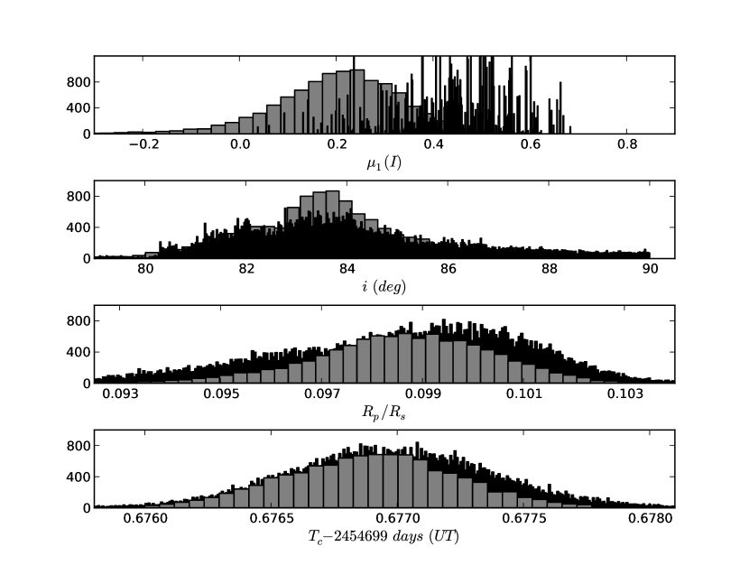
Figure 2 shows the distribution of each parameter obtained using the LMMC and the MCMC techniques with data from 2008-08-21 transit (similar analysis was done with the other 6 complete light curves). From the three bottom panels in the Figure 2 it is evident that the errors (defined as the 68% of a Gaussian fit to the parameter value distributions) obtained with LMMC are generally smaller than those obtained using MCMC, since the latter does a more exhaustive exploration of the parameter space and therefore performs better error estimations. Also, from the top-panel of Figure 2, it can be seen that the LMMC results for certain parameters can appear biased towards their initial input values. That is the case for the linear limb-darkening coefficient, for which the value resulting from the LMMC analysis is (the initial value was 0.296). On the other hand, the distribution of values for this parameter on a single epoch as given by MCMC does not appear Gaussian, revealing that the quality of a single transit in the current data does not allow to constrain the values of . Notice, however, that a Gaussian distribution is obtained when fitting several transits simultaneously (see Figure 4 and section 3.2).
From the test results above we conclude that the LMMC and MCMC techniques arrive to similar parameter results. However, because the apparent underestimation of the errors estimated by LMMC we have opted for using TAP for our analysis of the full WASP-5b (catalog ) transit dataset and the re-analysis of all the available data (see next section). This underestimation is due to lack of multi-parameter uncertainty estimator and failure to account for red noise in the minimization (Carter & Winn 2009) as TAP does. Other advantages of TAP include that the code can fit a greater number of parameters like linear systematics in the datasets, and it allows a simultaneous fitting of multiple transits.
3.2 Final Modeling
We used TAP to fit the nine new transit light curves presented in this paper and all the available light curves of the system (seven of F11, two of D11, two of S09 and the two of A08).
First, we attempted to model each of the new light curves independently, but ran into several problems. TAP had difficulties fitting the incomplete light curves. Also, when fitting individual light curves, parameters such as did not clearly converge to a single value, as already mentioned in section 3.1 and illustrated in Figure 2. To avoid these problems we fit the seven complete light curves simultaneously, leaving as free parameters , , , , , in addition to possible linear trends to the light curves, , and white (uncorrelated) and red (correlated) noise components, and , respectively. The orbital period, the eccentricity, and the longitude of the periastron were fixed to the values P= 1.62843142 days (the value obtained by F11), and .
We used a quadratic limb-darkening law, but found that the precision of the light curves was not enough to reliably fit the quadratic coefficient, so that value was also fixed to , based on the tabulated results in Claret (2000).
As mentioned in Section 2, we initially corrected for systematic trends in the light curves using linear or quadratic regression fits. Altough slopes in the light curves are not clearly apparent, we leave and as free parameters to ensure that any small residuals are properly fit. This might create concerns about wheter this two-step fitting of systematics can affect the results of the fits. To ensure we are not introducing any bias on the determination of the planetary parameters, we fit the two sets of data (i.e. the light curves with and without systematics trends removed) with TAP and arrive to consistent values of all derived planetary parameters.
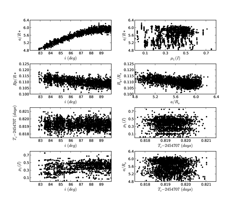
We also searched for potential parameter correlations in the light curves using the fit results of the 2008-08-29 transit described in the previous section, where all the parameters were let to vary. The resultant parameter correlations are shown in Figure 3. This figure reveals a strong correlation between and . There is also evidence of weaker correlations between those two parameters and . Therefore, to minimize the impact of those correlations in our results, we fixed in all the light curves to 5.37 (from F11), while closely monitoring and for variations.
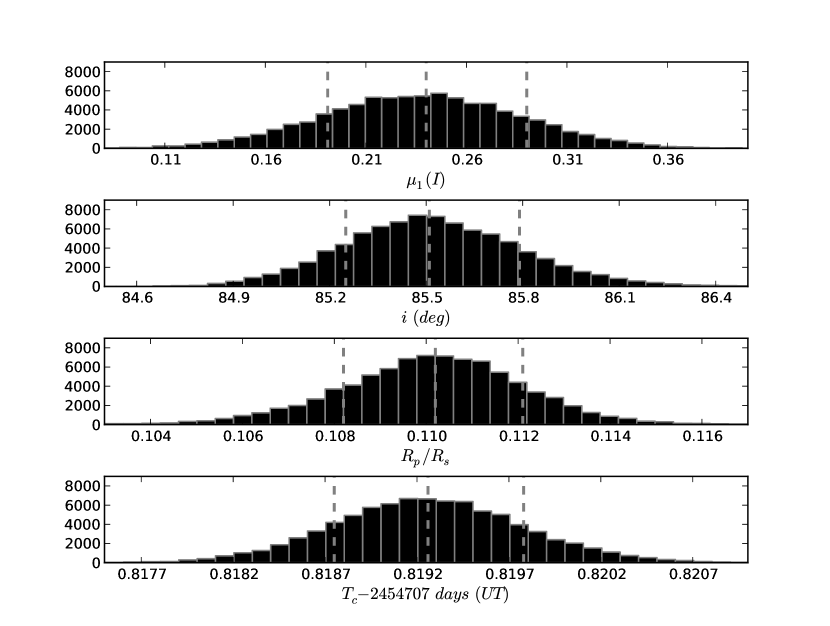
To fit the transits we ran 10 MCMC chains of links each, discarding the first 10% results from each chain to avoid bias toward the initial input values of each fitted parameter. Because the resulting MCMC distributions for are not Gaussian (see Figures 2 and 3), that parameter was fit simultaneously for all seven light curves, while for the other parameters we obtained one value per curve and combine them afterward via a weighted average. The resulting average values for each parameter are listed in Table 3, together with their 1 errors. As an example, Figure 4 shows the resultant MCMC distributions of , , and for the transit observed on 2008-08-29, while the distribution of correspond to the results of the simultaneous seven transits fit. This distribution is now clearly Gaussian in contrast with the previously obtained.
Finally, we adopted the values of all the parameters that define the shape of the transit derived in the fit above and used them as fixed values in the two incomplete light curves (2008-10-22 and 2009-08-06 transits) to derive their mid-times of transit, . The , , and are still left variable in this case.
F11 used a procedure based on minimization for modeling their light curves. We re-analyzed their data to do an homogeneous study of all the light curves, given that a multi-parameter minimization based on MCMC is statistically more robust. We modeled the seven light curves of F11555The data is available in the on-line material from the F11 publication on PASJ, the two light curves of D11 (data provided by the author, private communication), the two light curves of S09666The data is available at the CDS (http://cdsweb.u-strasbg.fr/) and the two of A08 (data provided by the author, private communication) in a similar manner to our complete light curves above. The F11 transits were observed with a Bessel I filter, the D11 and the S09 with a filter, and the A08 with and SDSS i’ filter; therefore, we fit one simultaneously for all F11 curves, one for the D11 curves and one for the S09 curves, and separate and for the A08 curves. We fixed in all cases.
The obtained parameters are summarized Table 3. The resultant models to all 22 light curves are illustrated in Figure 1.
We point out that the errors of the F11’s light curves estimated by us are, in average, larger than the reported by F11. We checked that the origin of this difference was not due only by the different red-noise estimator methods. Using the same red-noise factor estimated by F11, we have obtained errors consistent with those we present in Table 3. Carter & Winn (2009) found that time averaging and residual permutation methods underestimated the errors by compared with the wavelet-based method (implemented by TAP).
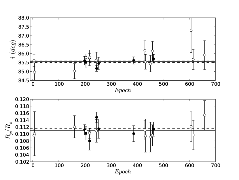
Using the model results is possible to look for variations in the most relevant parameters, in particular and , that can reveal the presence of an additional body in the system. In Figure 5, we plot and as a function of the transit epoch, based in the results of the twenty transit fits (our two incomplete light curves were not included). We do not see any significant variations in those parameters. The weighted average values of and based on all the light curves results are summarized in Table 4. We studied in detail the timing of the transits in the next section.
4 Timing Analysis
The times in our nine transit data and the D11 data were initially computed in Coordinated Universal Time (UTC) and then converted to Barycentric Julian Days, expressed in Terrestrial Time, BJD(TT), using the Eastman et al. (2010) online calculator 777http://astroutils.astronomy.ohio-state.edu/time/utc2bjd.html. The transit times of S09 and A08, which were initially expressed in HJD(UT) have also been converted to BJD(TT). No conversion was applied to the light curves reported by F11.
The times of the common transits, 2008-08-29 and 2008-09-21, derived from our light curves are consistent within the errors in the values derived by us and also by F11 from S09 data.
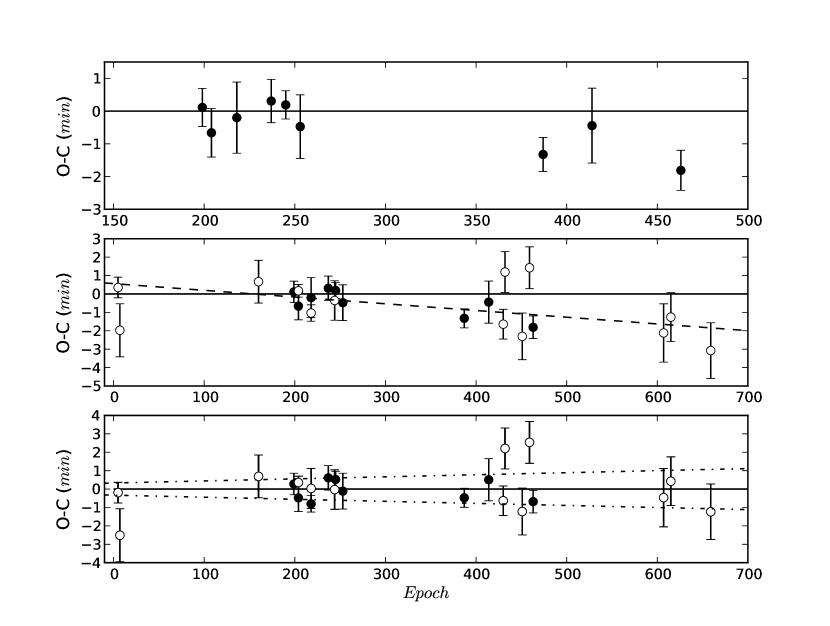
Using the F11’s ephemeris equation, we calculated the residuals of the mid-times of the 22 transits of WASP-5b (catalog ) analyzed in this work. The top panel in Figure 6, shows the () diagram for our nine transits. In the middle panel of the figure we combine the values of our nine transits with the new values derived for the F11, D11, S09 and A08 (shown as open circles). As illustrated in that figure, a linear trend with a slope of days is observed in the time residuals of all transits. That trend can be explained by the accumulation of errors in the current orbital period and of the transits over time, and therefore can be modeled out.
This linear regression of the points in the diagram has a ( for 20 degrees of freedom), which is significantly smaller than the value obtained for F11 of ( for 9 degrees of freedom). Additionally, we confirmed that with our results for the 11 epochs included in F11’s analysis we also obtained an smaller ( that yields ). This result lies in the fact that our uncertainties are larger than those estimated by F11.
Once the linear trend is removed the updated ephemeris equation is:
where is the central time of a transit in the epoch since the reference time . The errors of the last digits are shown in parenthesis. The bottom panel in Figure 6 shows the resulting values of all available transits using the updated ephemeris equation. The resultant diagram is consistent with a constant period, and we conclude that the observed TTV residuals (with a RMS of days seconds), are most likely introduced by data uncertainties and systematics rather than due by gravitational perturbations of an orbital companion. This newly obtained precision permits to place strong constraints in the mass of an hypothetical companion, particularly in MMR’s, as we discuss in the next section.
5 Limits to additional planets
To place upper limits to the potential perturbers in the WASP-5 (catalog ) system based in the derived TTV RMS of about 60 sec we use Mercury (Chambers 1999) N-body simulator. The input parameters to include the mass and the radius of both the star and the transiting planets, the planet-to-star orbital separation, as well as the inclination, eccentricity and periastron longitude of the system. The values for all these parameters were adopted from S09. In addition, all the initial relative angles between the perturber and WASP-5b (catalog ) were set to zero.
We explored a wide range of perturber masses between and in initial steps of , which are subsequently refined as described below. For the semi-major axis distances we explore a range between 0.001 and 1.2 AU in steps of 0.001 AU, which was further reduce near resonances. The density of the perturber was kept constant to that of Earth for and to that of Jupiter for , it was varied linearly for masses in between. Also, we assumed the perturber to be in a circular orbit and coplanar to WASP-5b (catalog ), since this configuration provides the most strict limit to the amplitude of the TTVs for a given perturber’s mass. Non-zero eccentricities and non-coplanar orbits produce larger TTVs as already pointed out by e.g. Bean (2009), Hoyer et al. (2011) and Fukui et al. (2011). For each model configuration we let the system relax for five years, and then we used the next five years to obtain our fit results, which in total is more than 3 times the time span of the observations. These 5 years of relaxation time permits to minimize the effect of any initial bias (e.g. the relative angles). We found orbits between 0.02 and 0.035 AU to be unstable due to the presence of WASP-5b. For all other (stable) orbits we recorded the central times of each transit of WASP-5b and computed the predicted TTVs for each configuration, assuming an average constant period. Additionally, we checked that the fitted average period did not deviate by more than from the obtained orbital period of WASP-5b (catalog ). Also, to ensure a good sampling of the potential perturber’s mass, we reduced the steps in to whenever the TTVs approached 60 sec.
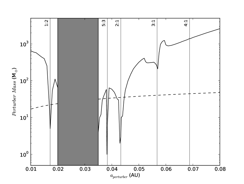
The results of our model simulations is illustrated in Figure 7, where we show the () versus diagram that places the mass limits to potential perturbers in the system. The solid line in the diagram indicates the derived upper limits to the mass of the perturbers that would produce TTVs RMS of sec at different orbital separation. The dashed line shows the perturber mass upper limits imposed by the most recent radial velocity observations of the WASP-5 system, for which we have adopted a precision of 15 m/s (A08 and Triaud et al. 2010, report RV precision of 14 m/s and m/s, respectively).
Figure 7 thus shows that the perturber would have been detected by RV measurements in all areas except around the 1:2, 5:3 and 2:1 MMRs, where it could have a maximum mass of 5, 1 and 2 , respectively.
6 Conclusions
We present nine new transit light curves of WASP-5b (catalog ). We homogeneously model these light curves together with all available transit data of this system. Based in these fits we search for any variation in the timing of the transits.
Using 22 transit epochs we updated the ephemeris equation and we find a TTVs RMS of seconds. All the transit times are consistent with a constant orbital period within 2.
Our linear fit of the transit times has a , which is considerably lower than the value found by Fukui et al. (2011) used to implied the presence of an perturber body.
Despite obtaining a similar TTV RMS than Fukui et al. (2011) ( min), we conclude a much smaller significance to deviations from a constant period due to our larger per-epoch uncertainties as obtained by the MCMC algorithm.
If the system has an additional orbiting body, its mass has to be lower than 5, 1 and 2 , in the 2:1, 5:3 and 1:2 resonances. In any other location the perturber would have been detected by RVs.
We search for any trend in the depth of the transit and inclination of the orbit but we do not see any clear evidence of variation with statistical significance.
7 Acknowledgements
The authors would like thank David Anderson for providing WASP light curves and Diana Dragomir and Stephen Kane for providing TERMS light curves. S.H. and P.R. acknowledgements support from Basal PFB06, Fondap #15010003, and Fondecyt #11080271. Additionally, S.H, recieved support from ALMA-CONICYT FUND #31090030. We thanks the CTIO and SOAR staff for the help and continuous support during the numerous observing nights.
References
- Adams et al. (2010) Adams, E. R., López-Morales, M., Elliot, J. L., Seager, S., & Osip, D. J. 2010, ApJ, 714, 13
- Agol et al. (2005) Agol, E., Steffen, J., Sari, R., & Clarkson, W. 2005, MNRAS, 359, 567
- Anderson et al. (2008) Anderson, D. R., et al. 2008, MNRAS, 387, L4
- Bean (2009) Bean, J. L. 2009, A&A, 506, 369
- Carter & Winn (2009) Carter, J. A., & Winn, J. N. 2009, ApJ, 704, 51
- Chambers (1999) Chambers, J. E. 1999, MNRAS, 304, 793
- Claret (2000) Claret, A. 2000, A&A, 363, 1081
- Dragomir et al. (2011) Dragomir, D., et al. 2011, ArXiv e-prints
- Eastman et al. (2010) Eastman, J., Siverd, R., & Gaudi, B. S. 2010, PASP, 122, 935
- Ford et al. (2011) Ford, E. B., et al. 2011, ArXiv e-prints
- Fukui et al. (2011) Fukui, A., et al. 2011, PASJ, 63, 287
- Fulton et al. (2011) Fulton, B. J., Shporer, A., Winn, J. N., Holman, M. J., Pál, A., & Gazak, J. Z. 2011, ArXiv e-prints
- Gazak et al. (2011) Gazak, J. Z., Johnson, J. A., Tonry, J., Eastman, J., Mann, A. W., & Agol, E. 2011, ArXiv e-prints
- Gillon et al. (2009) Gillon, M., et al. 2009, A&A, 496, 259
- Holman & Murray (2005) Holman, M. J., & Murray, N. W. 2005, Science, 307, 1288
- Holman et al. (2010) Holman, M. J., et al. 2010, Science, 330, 51
- Hoyer et al. (2011) Hoyer, S., Rojo, P., López-Morales, M., Díaz, R. F., Chambers, J., & Minniti, D. 2011, ApJ, 733, 53
- Kipping (2009) Kipping, D. M. 2009, MNRAS, 392, 181
- Latham et al. (2011) Latham, D. W., et al. 2011, ApJ, 732, L24+
- Lissauer et al. (2011) Lissauer, J. J., et al. 2011, Nature, 470, 53
- Miguel et al. (2011) Miguel, Y., Guilera, O. M., & Brunini, A. 2011, MNRAS, 417, 314
- Miralda-Escudé (2002) Miralda-Escudé, J. 2002, ApJ, 564, 1019
- Naoz et al. (2011) Naoz, S., Farr, W. M., Lithwick, Y., Rasio, F. A., & Teyssandier, J. 2011, Nature, 473, 187
- Sartoretti & Schneider (1999) Sartoretti, P., & Schneider, J. 1999, A&AS, 134, 553
- Smith et al. (2009) Smith, A. M. S., et al. 2009, MNRAS, 398, 1827
- Southworth (2010) Southworth, J. 2010, MNRAS, 408, 1689
- Southworth et al. (2004a) Southworth, J., Maxted, P. F. L., & Smalley, B. 2004a, MNRAS, 351, 1277
- Southworth et al. (2004b) Southworth, J., Zucker, S., Maxted, P. F. L., & Smalley, B. 2004b, MNRAS, 355, 986
- Southworth et al. (2009) Southworth, J., et al. 2009, MNRAS, 396, 1023
- Triaud et al. (2010) Triaud, A. H. M. J., et al. 2010, A&A, 524, A25+
| Transit Date | Telescope/Instrument | Filter | Integration Time [s] | airmass range | Epoch |
|---|---|---|---|---|---|
| 2008-08-21 | SMARTS-1m/Y4KCam | Bessell I | 13 | 1.7 - 1.01 | 199 |
| 2008-08-29aaThis transit was also observed by Southworth et al. (2009). | SMARTS-1m/Y4KCam | Bessell I | 10 | 1.05 - 1.02 - 1.06 | 204 |
| 2008-09-21aaThis transit was also observed by Southworth et al. (2009). | SMARTS-1m/Y4KCam | Bessell I | 10,7 | 1.9 - 1.01 - 1.07 | 218 |
| 2008-10-22bbThis transit has a incomplete phase coverage. | SOAR/SOI | Bessell I | 7,5,3 | 1.12 - 1.02 | 237 |
| 2008-11-04 | SOAR/SOI | Bessell I | 3 | 1.07 - 1.02 - 1.4 | 245 |
| 2008-11-17 | SMARTS-1m/Y4KCam | Bessell I | 10 | 1.02 - 1.4 | 253 |
| 2009-06-22 | SOAR/SOI | Bessell I | 7,5,3 | 1.95 - 1.02 | 387 |
| 2009-08-06bbThis transit has a incomplete phase coverage. | SOAR/SOI | Bessell I | 5,4 | 1.07 - 1.15 | 414 |
| 2009-10-25 | SMARTS-1m/Y4KCam | Bessell I | 15 | 1.06 - 1.02 - 1.97 | 463 |
| Parameter | JKTEBOP | TAP |
|---|---|---|
| () | ||
| Transit date | Epoch | aaIn all the fits the quadratic coefficient was fixed to . | () | / | ||
|---|---|---|---|---|---|---|
| 2008-08-21 | 199 | 1.6 | ||||
| 2008-08-29 | 204 | 2.8 | ||||
| 2008-09-21 | 218 | 2.9 | ||||
| 2008-10-22 | 237 | bbThese parameters were fixed in the modeling and correspond to the weighted average of the results of the other seven full phase covered light curves presented in this work. | bbThese parameters were fixed in the modeling and correspond to the weighted average of the results of the other seven full phase covered light curves presented in this work. | bbThese parameters were fixed in the modeling and correspond to the weighted average of the results of the other seven full phase covered light curves presented in this work. | 2.3 | |
| 2008-11-04 | 245 | 5.3 | ||||
| 2008-11-17 | 253 | 2.5 | ||||
| 2009-06-22 | 387 | 10.3 | ||||
| 2009-08-06 | 414 | bbThese parameters were fixed in the modeling and correspond to the weighted average of the results of the other seven full phase covered light curves presented in this work. | bbThese parameters were fixed in the modeling and correspond to the weighted average of the results of the other seven full phase covered light curves presented in this work. | bbThese parameters were fixed in the modeling and correspond to the weighted average of the results of the other seven full phase covered light curves presented in this work. | 8.2 | |
| 2009-10-25 | 463 | 5.6 | ||||
| 2008-06-18ccfootnotemark: | 160 | 2.9 | ||||
| 2008-11-02ccfootnotemark: | 244 | 2.2 | ||||
| 2009-09-04ccfootnotemark: | 432 | 2.0 | ||||
| 2009-10-05ccfootnotemark: | 451 | 10.1 | ||||
| 2009-10-18ccfootnotemark: | 459 | 2.5 | ||||
| 2010-06-16ccfootnotemark: | 607 | 4.9 | ||||
| 2010-06-29ccfootnotemark: | 615 | 5.2 | ||||
| 2009-09-01ddfootnotemark: | 430 | 8.0 | ||||
| 2010-09-09ddfootnotemark: | 659 | 4.6 | ||||
| 2008-08-29eefootnotemark: | 204 | 3.0 | ||||
| 2008-09-21eefootnotemark: | 218 | 3.7 | ||||
| 2007-10-10fffootnotemark: | 5 | 4.9 | ||||
| 2007-10-13fffootnotemark: | 7 | 11.7 |
| Parameter | Adopted Value | Error |
|---|---|---|
| aaValue and error adopted from Fukui et al. (2011). | ||
| Period [days] | ||
