An Analytic Formula for the Supercluster Mass Function

Abstract

We present an analytic formula for the supercluster mass function which is constructed by modifying the extended Zel’dovich model for the halo mass function. The formula has two characteristic parameters whose best-fit values are determined by fitting to the numerical results from N-body simulations for the standard $\Lambda$CDM cosmology. The parameters are found to be independent of redshifts and robust against variation of the key cosmological parameters. Under the assumption that the same formula for the supercluster mass function is valid for non-standard cosmological models, we show that the relative abundance of the rich superclusters should be a powerful indicator of any deviation of the real universe from the prediction of the standard $\Lambda$CDM model.

1 INTRODUCTION

The gravitational aggregates of (a few to hundreds of) galaxy clusters are called the superclusters which are marginally bound systems. Although quite rare in the local universe, the superclusters are believed to be common phenomena on the scales larger than $100$ Mpc. The nearby Virgo cluster as well as the Local Group where our Milky Way resides also belongs to the Local Supercluster that contains more than $100$ member clusters (Tully, 1982, and references there in).

In the standard $\Lambda$CDM ($\Lambda$+cold dark matter) universe, the formation of the superclusters at the present epoch represents the grand finale of the hierarchical merging events. No bound objects could form on mass scale larger than that of the present rich superclusters in the future due to the anti-gravitational effect of the cosmological constant ($\Lambda$). That is, the rich superclusters observed at the present epoch will end up as isolated massive clusters in the future when $\Lambda$ becomes progressively more dominant (e.g., see Nagamine & Loeb, 2003; Kasun & Evrard, 2005; Busha et al., 2005; Araya-Melo et al., 2009).

If the dark energy were not $\Lambda$ or if the large-scale gravity deviated from the general relativity (GR), the superclusters could meet a different fate. For example, in QCDM (Quintessence+CDM) models, more massive objects than the rich superclusters would form through the large scale clustering of the Quintessence scalar field (see Caldwell et al., 1998, and references therein). In some modified gravity scenarios where the universe has no anti-gravitational dark energy (for a review, see Clifton et al., 2012), nothing would prevent the superclusters from assembling into larger scale objects. Henceforth, the abundance of rich superclusters might be a powerful indicator of any deviation of the real universe from the prediction of the standard $\Lambda$CDM model.

There are two advantages that the number count of rich superclusters has as a cosmological probe over that of the clusters. First of all, the rich superclusters are larger and rarer on average than the clusters, and thus their abundance should be more sensitive to the background cosmology. The other advantage is that since the superclusters are still in the quasi-linear regime, their formation process would be less affected by the complicated nonlinear effect and thus their mass function (defined as the number density of the superclusters per unit volume as a function of mass) may be easier to model theoretically.

It was Oguri et al. (2004) who for the first time attempted to find an analytic expression for the supercluster mass function in the framework of the standard Press-Schechter theory (Press & Schechter, 1974). Pioneering as it was, their work was based on a few unjustified assumptions, which resulted in the failure of their model in matching the N-body results (M. Oguri in private communication). Yan & Fan (2011) determined numerically the mass function of the supercluster-like filaments with the help of large N-body simulations and showed that the standard excursion set theory is incapable of reproducing the numerical results. Although they claimed that the incorporation of the ”peak-exclusion effect” could lead the excursion set mass function to match qualitatively the numerical results, their model could not pull it off quantitatively.

Our goal here is to find an efficient analytic formula for the supercluster mass function by modifying the extended Zel’dovich (EZL) model for the halo mass function which was constructed in our previous work (Lim & Lee, 2013). The EZL model is based on the formalism originally developed by Jedamzik (1995) and characterized by three parameters expressed in terms of the thresholds of the linear shear eigenvalues. As mentioned clearly in Lim & Lee (2013), the EZL model is not a physical model but a fitting formula whose characteristic parameters have to be determined empirically by adjusting the model to numerical results. Nevertheless, it turned out that the best-fit parameters of the EZL model are independent of redshift, having the same values even when the background cosmology changes. Furthermore, the EZL formula for the halo mass function was shown to agree with the N-body results better than the other analytic formula suggested so far (e.g., Sheth & Tormen, 1999; Tinker et al., 2008; Pillepich et al., 2010), which encourages us to use it as a basic framework for the analytic construction of the supercluster mass function.

This Paper is composed of five sections whose contents are outlined as follows: In section 2 we provide a brief review of the EZL model and describe how the EZL model is modified to construct a new formula for the supercluster mass function. In section 3 we compare our model with the numerical results from three different N-body simulations. In section 4 we explore the possibility of using the relative abundance of rich superclusters as a new cosmological probe. In section 5 we discuss the results and assess its cosmological importance.

2 CONSTRUCTING A SUPERCLUSTER MASS FUNCTION

2.1 Summary of the EZL model

The EZL model for the differential mass function of bound halos, $dN/dM$, is expressed by the following integral equation

$$F(\lambda_{1c},\lambda_{2c},\lambda_{3c};M)=\int_{M}^{\infty}dM^{\prime}{M^{\prime}\over{\bar{\rho}}}\frac{dN}{dM^{\prime}}P(M,M^{\prime})\ ,$$ (1)

which look similar to the formula originally developed by Jedamzik (1995). The key difference of equation (1) from the original Jedamzik formula is that the characteristic parameters of the EZL model are expressed in terms of the thresholds (i.e., lower limits) of three eigenvalues of the linear deformation tensor, $\lambda_{1c},\ \lambda_{2c},\ \lambda_{3c}$.

The left-hand side in equation (1) is equal to the cumulative probability that the linear shear eigenvalues $\lambda_{1},\ \lambda_{2},\ \lambda_{3}$ (with $\lambda_{1}\geq\lambda_{2}\geq\lambda_{3}$) on the mass scale $M$ exceed their thresholds:

$$F(M) = P[\lambda_{1}\geq\lambda_{1c},\lambda_{2}\geq\lambda_{2c},\lambda_{3}\geq\lambda_{3c}|\sigma(M)]\,,$$ (2)

$$= \int^{\infty}_{\lambda_{1c}}d\lambda_{1}\,\int^{\lambda_{1}}_{\lambda_{2c}}d\lambda_{2}\,\int^{\lambda_{2}}_{\lambda_{3c}}d\lambda_{3}\,p[\lambda_{i};\sigma(M)],$$ (3)

where $\sigma(M)$ is the rms fluctuation of the linear density contrast smoothed by a top-hat filter on the mass scale of $M$. Equation (3) can be straightforwardly calculated from the joint probability density distribution of the linear shear eigenvalues derived by Doroshkevich (1970)

$$p(\lambda_{1},\lambda_{2},\lambda_{3})=\frac{3375}{8\sqrt{5}\pi\sigma^{6}}\exp\left[-\frac{3}{\sigma^{2}}\left(\sum_{i=1}^{3}\lambda_{i}\right)^{2}+\frac{15}{2\sigma^{2}}\sum_{i>j}\lambda_{i}\lambda_{j}\right]|\Pi_{i>j}(\lambda_{i}-\lambda_{j})|,$$ (4)

The core quantity in the right-hand side of equation (1) is the conditional probability $P(M,M^{\prime})$ defined as

$$P(M,M^{\prime})\equiv\int_{\lambda_{1c}}^{\infty}d\lambda_{1}\int_{\lambda_{2c}}^{\lambda_{1}}d\lambda_{2}\int_{\lambda_{3c}}^{\lambda_{2}}d\lambda_{3}\,p_{c}(\lambda_{i}|\lambda^{\prime}_{i}=\lambda_{ic})\,$$ (5)

where $p_{c}(\lambda_{i}|\lambda^{\prime}_{i}=\lambda_{ic})$ is the conditional joint probability density evaluated as

$$p_{c}(\lambda_{1},\lambda_{2},\lambda_{3}|\lambda^{\prime}_{1}=\lambda_{1c},\lambda^{\prime}_{2}=\lambda_{2c},\lambda^{\prime}_{3}=\lambda_{3c})=\frac{p(\lambda_{1},\lambda_{2},\lambda_{3},\lambda^{\prime}_{1}=\lambda_{1c},\lambda^{\prime}_{2}=\lambda_{2c},\lambda^{\prime}_{3}=\lambda_{3c})}{p(\lambda^{\prime}_{1}=\lambda_{1c},\lambda^{\prime}_{2}=\lambda_{2c},\lambda^{\prime}_{3}=\lambda_{3c})}\,.\$$ (6)

where $\{\lambda^{\prime}_{i}\}_{i=1}^{3}$represent the shear eigenvalues on some larger mass scale $M^{\prime}\geq M$.

Equations (5)-(6) require to have the joint probability density distribution of the shear eigenvalues on two different mass scales, $M$ and $M^{\prime}$, which have been already analytically found in the ingenious works of Desjacques (2008) and Desjacques & Smith (2008):

$$p(\lambda_{1},\lambda_{2},\lambda_{3},\lambda^{\prime}_{1},\lambda^{\prime}_{2},\lambda^{\prime}_{3}) = \frac{15^{6}}{320\pi^{2}\sigma^{6}\sigma^{\prime 6}}(1-\gamma^{2})^{-3}w(\beta\epsilon_{-},\epsilon_{\lambda^{\prime}},\epsilon_{\lambda})\mathrm{e}^{-Q+\beta\epsilon_{+}}\times\,$$ (8)

$$|\Pi_{i>j}(\lambda_{i}-\lambda_{j})\Pi_{i>j}(\lambda^{\prime}_{i}-\lambda^{\prime}_{j})|.$$

$$\gamma = \frac{1}{2\pi^{2}\sigma\sigma^{\prime}}\int_{0}^{\infty}{d(\ln k)k^{3}P(k)W(k;M)W(k;M^{\prime})}\,,$$

$$\beta = \frac{15\gamma}{2(1-\gamma^{2})}\,,$$

$$Q = \frac{3}{4(1-\gamma^{2})}\left\{5[\mathrm{tr}(\lambda^{\prime 2})+\mathrm{tr}(\lambda^{\prime 2})]-(\mathrm{tr}\lambda^{\prime})^{2}-(\mathrm{tr}\lambda)^{2}+2\gamma(\mathrm{tr}\lambda^{\prime})(\mathrm{tr}\lambda)\right\}\,,$$

$$w = \frac{\mathrm{e}^{-\beta\epsilon_{-}}}{2\pi}\int_{0}^{1}{dr}\int_{0}^{2\pi}{d\varphi\exp\Bigg{[}\frac{3\beta\epsilon_{-}}{4}g\Bigg{]}I_{0}\Bigg{[}\frac{3\beta\epsilon_{-}\epsilon_{\lambda}}{4}\sqrt{h}\Bigg{]}}\,,$$ (9)

where $g$ and $h$ are given as

$$g = 1+r^{2}+\epsilon_{\lambda^{\prime}}(1-r^{2})\cos(2\varphi)\,,$$ (10)

$$h = g^{2}-4(1-\epsilon_{\lambda^{\prime}}^{2})r^{2}\,,$$ (11)

and $\sigma^{\prime}\equiv\sigma(M^{\prime})$, $\sigma\equiv\sigma(M)$, and

$$\mathrm{tr}\lambda^{\prime}=\sum_{i}{(\lambda^{\prime}/\sigma^{\prime})},\ \mathrm{tr}\lambda=\sum_{i}{(\lambda/\sigma)},$$ (12)

$$\mathrm{tr}(\lambda^{\prime 2})=\sum_{i}{(\lambda^{\prime}/\sigma^{\prime})^{2}},\ \mathrm{tr}(\lambda^{2})=\sum_{i}{(\lambda/\sigma)^{2}},\$$ (13)

$$\epsilon_{+}=\frac{1}{3}(\mathrm{tr}\lambda^{\prime})(\mathrm{tr}\lambda),\$$ (14)

$$\epsilon_{-}=\frac{1}{3}(\mathrm{tr}\lambda^{\prime}-3\lambda_{3}^{\prime}/\sigma^{\prime})(\mathrm{tr}\lambda-3\lambda_{3}/\sigma),\$$ (15)

$$\epsilon_{\lambda^{\prime}}=(\lambda_{1}^{\prime}-\lambda_{2}^{\prime})/(\mathrm{tr}\lambda^{\prime}-3\lambda_{3}^{\prime}/\sigma^{\prime}),\$$ (16)

$$\epsilon_{\lambda}=(\lambda_{1}-\lambda_{2})/(\mathrm{tr}\lambda-3\lambda_{3}/\sigma).$$ (17)

Rewriting equation (1) as a discrete matrix equation and solving it through equations (2)-(17), Lim & Lee (2013) obtained the halo mass function, $dN/dM$ and determined the best-fit values of $\{\lambda_{1c},\ \lambda_{2c},\ \lambda_{3c}\}$ by adjusting the EZL model to the numerical results. As mentioned in section 1, the EZL mass function of bound halos turned out to be in excellent agreements with N-body results and the best-fit values of $\{\lambda_{1c},\ \lambda_{2c},\ \lambda_{3c}\}$ were shown to be independent of redshifts and the background cosmology.

2.2 Modification of the EZL model

To construct a new formula for the supercluster mass function by modifying the EZL model, we first modify the LHS of equation (1) into

$$F(M) \propto P[\lambda_{1}\leq\lambda_{1c},\lambda_{2}\geq\lambda_{2c},\lambda_{3}\geq 0|\sigma(M)]\,,$$ (18)

$$\propto \int^{\lambda_{1c}}_{\lambda_{2c}}d\lambda_{1}\,\int^{\lambda_{1}}_{\lambda_{2c}}d\lambda_{2}\,\int^{\lambda_{2}}_{0}d\lambda_{3}\,p[\{\lambda_{i}\};\sigma(M)],$$ (19)

where the largest shear eigenvalue, $\lambda_{1}$, has an upper limit rather than a lower limit unlike in equation (3) and the lower limit of the smallest eigenvalue, $\lambda_{3}$, is fixed at zero. Our new formula for the supercluster mass function has two characteristic parameters, $\lambda_{1c}$ and $\lambda_{2c}$, which represent the lower and the upper limit sof the largest and the second to the largest eigenvalues of the linear deformation tensor, respectively.

The conditional probability, $P(M,M^{\prime})$, in the RHS of equation (1) is accordingly modified into

$$P(M,M^{\prime})=\int_{\lambda_{2c}}^{\lambda_{1c}}d\lambda_{1}\int_{\lambda_{2c}}^{\lambda_{1}}d\lambda_{2}\int_{0}^{\lambda_{2}}d\lambda_{3}\,p_{c}(\lambda_{i}|\lambda^{\prime}_{i}=\lambda_{ic})\,$$ (20)

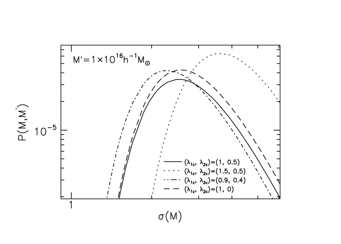
Figure 1 plots this conditional probability distribution versus the rms density fluctuation for four different cases of the characteristic parameters, $\lambda_{1c}$ and $\lambda_{2c}$. As can be seen, the conditional probability distribution, $P(M,M^{\prime})$, sensitively changes as the values of the characteristic parameters change.

As done in Lim & Lee (2013), rewriting equation (1) as a discrete matrix equation and solving it for $dN/dM$ through equations (18)-(20), one can obtain the differential mass function of the marginally bound superclusters, $dN/dM$. It is, however, worth noting here that unlike the case of bound halos where the EZL formula yields an automatically normalized mass function, for the case of the superclusters the modified EZL formula has to be renormalized to satisfy the following condition.

$$\int_{M_{\rm c,th}}dM\ \frac{dN}{dM}=\frac{N_{\rm T}}{V_{\rm T}}\,,$$ (21)

where $N_{\rm T}$ denotes the total number of superclusters with mass larger than $M_{\rm c,th}$ found in the volume of $V_{\rm T}$ (see section 3). Equation (21) will be used to determine the value of the proportionality constant (i.e., normalization factor) in equation (18). This renormalization step is necessary since not all initial regions would form marginally bound superclusters in the end.

We would like to state explicitly here that this modified EZL formula for the supercluster mass function is not a physical model and the characteristic parameters, $\{\lambda_{1c},\ \lambda_{2c},\ \lambda_{3c}\}$, are not related to any underlying dynamics but should be determined by numerical experiments. In other words, we note only empirically that the modification of Equation (3) into Equation (19) works for the case of the supercluster mass function.

3 NUMERICAL TESTS

To test our model for the supercluster mass function against the numerical results, we utilize three different N-body simulations: the Millennium (Springel et al., 2005), the CoDECS (Baldi, 2012) and the MICE (Crocce et al., 2010) simulations, all of which ran for a flat $\Lambda$CDM cosmology but with slightly different cosmological parameters . Table 1 lists the linear size of the simulation box, mass resolution, total number of particles, values of the three key cosmological parameters, and the halo-finding algorithm used for the three simulations. The Friends-of-Friends (FoF) algorithm with linking length of $0.2\bar{l}_{p}$ (where $\bar{l}_{\rm p}$ is the mean particle separation) was used in all of the simulations to find the bound groups of dark matter particles. See the above three literatures for the full descriptions of the simulations and the halo-identification procedure.

The publicly available halo catalogs from each simulation provide such information on the resolved halos as their mass, positions, velocities and so forth at various redshifts. Analyzing the catalogs from each simulation at three different redshifts ($z=0,\ 0.5,\ 1$ for the cases of the Millennium and MICE catalogs while $z=0,\ 0.44,\ 1$ for the case of the CoDECS catalog), we first construct a mass-limited sample of the clusters from each catalog which includes only those halos with masses larger than a threshold value, $M_{\rm c,th}=10^{13}\,h^{-1}M_{\odot}$. For the case of the MICE halo catalogs, however, a slightly higher threshold value, $M_{\rm c,th}=3.4\times 10^{13}\,h^{-1}M_{\odot}$, is used since all of the halos in the MICE catalogs have masses larger than this higher threshold value.

Then, we identify the superclusters as the clusters of clusters by applying the FoF algorithm to the clusters in each mass-limited sample at each redshift. Following the conventional criterion suggested in the previous literatures (e.g., Kasun & Evrard, 2005; Wray et al., 2006; Lee & Evrard, 2007), we set the linking length of the FoF algorithm for the supercluster identification at $\bar{l}_{c}/3$ where $\bar{l}_{c}$ is the mean cluster separation.The mass of each identified supercluster, $M$, is measured as the sum of the masses of its member clusters. The total number and mean mass of the superclusters from the three simulations at three different redshifts are listed in Tables 2-4. Note that among the identified superclusters are included those which have only one member cluster (i.e., isolated clusters).

Binning the supercluster mass in the logarithmic scale, $\ln M$, and counting the number of the superclusters belonging to each differential mass bin, $[\ln M,\ \ln M+d\ln M]$, we determine the number density of the superclusters per unit volume, $dN/d\ln M$, as a function of $M$ at each redshift. To estimate the errors associated with the measurement of $dN/d\ln M$, we also perform the Jack-knife analysis: Dividing the superclusters into eight Jackknife subsamples, we determine $dN/d\ln M$ for each Jackknife subsample and calculate the one standard deviation scatter among the eight Jack-knife subsamples as the errors associated with the measurement of $dN/d\ln M$.

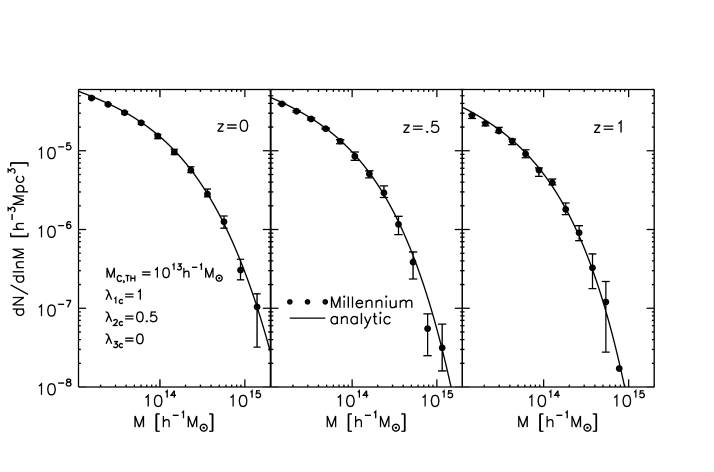
Now that the numerical results are all obtained, we want to compare them with the analytic formula constructed in section 2. With the help of $\chi^{2}$ minimization scheme, we first fit the numerical results from the Millennium simulation to the analytic supercluster mass function and determine the best-fit values of the two parameters to be $\lambda_{1c}=0.5$ and $\lambda_{2c}=0.5$, respectively, at $z=0$. Then, we examine whether or not the analytic model with the same best-fit values of the parameters still work at higher redshifts. For this comparison, the cosmological parameters are set at the same values that were used for the Millennium simulation when the analytic formula is calculated and the power spectrum of the standard $\Lambda$CDM is evaluated with the help of the CAMB code (Lewis et al., 2000).

Figure 2 plots the numerical results of the supercluster mass function from the Millennium simulations (solid dots) and compares them with the analytic models (solid line) with the best-fit parameters at $z=0,\ 0.5$ and $1$ in the left, middle and right panel, respectively. The supercluster mass function at higher redshifts can be readily evaluated just by substituting $\sigma(M,z)\equiv D(z)\sigma(M)$ for $\sigma(M)$ where $D(z)$ is the linear growth factor normalized to be unity at $z=0$. The functional form of $D(z)$ for a flat $\Lambda$CDM cosmology is given in Lahav et al. (1991). As can be seen in Figure 2, the analytic supercluster mass function with the same best-fit parameters agree excellently with the numerical results at all three redshifts.

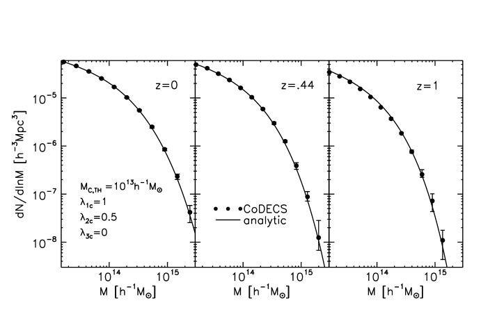
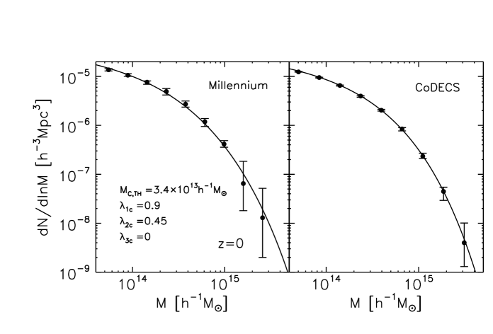
Due to the relatively small box size of the Millennium simulations (see Table 1), however, the numerical results in the high-mass section ($M\geq 10^{15}\,h^{-1}M_{\odot}$) suffer from large uncertainties. Figure 3 plots the same as Figure 2 but for the numerical results from the larger CoDECS simulations. The same values of the two parameters, $\lambda_{1c}=1$ and $\lambda_{2c}=0.5$, are consistently implemented into our formula while the key cosmological parameters are set at the values used for the CoDECS simulations. The analytic supercluster mass functions at three redshifts show excellent agreements with the numerical results from the CoDECS simulations, too.

Note that the value of the power spectrum amplitude is different between the two simulations as shown in Table 1: $\sigma_{8}=0.9$ for the Millennium while $\sigma_{8}=0.809$ for the CoDECS simulations. The excellent agreements between our formula and the numerical results from both of the simulations at three different redshifts indicate that the values of the two characteristic parameters should be independent of the background cosmology.

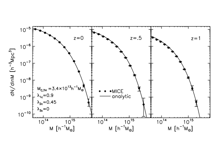
Figure 4 plots the same as Figure 2 but for the numerical results from the MICE simulations for which the $\chi^{2}$ statistics yield lower best-fit values of $\lambda_{1c}=0.9$ and $\lambda_{2c}=0.45$. Recall that a higher value of the mass threshold, $M_{\rm c,th}=3.4\times 10^{13}\,h^{-1}M_{\odot}$, is used to construct the mass-limited sample of the clusters from the MICE simulations. This higher value of $M_{\rm c,th}$ results in increasing the mean cluster separation, $\bar{l}_{c}$, which should in turn affect the best-fit values of the two parameters. Figure 4 reveals that our formula for the supercluster mass function agrees impressively well with the numerical results from the MICE simulations, too, even in the high-mass section ($M\geq 3\times 10^{15}\,h^{-1}M_{\odot}$) at all three redshifts.

Note that the mass-limited cluster sample from the MICE simulation contains less number of the low-mass clusters (i.e., the group-size clusters) than those from the other two simulations and thus it has a larger value of the mean cluster separation, $\bar{l}_{c}$. In other words, the identified superclusters via the FoF algorithm with the fixed linking length of $\bar{l}_{\rm c}/3$ must be less clustered. Henceforth, the values of the characteristic parameters of the EZL supercluster mass function, $\{\lambda_{1c},\ \lambda_{2c}\}$, should be related to the clustering strength among the member clusters of the superclusters.

We would like to examine whether or not the analytic model with the same lower values of $\{\lambda_{1c},\ \lambda_{2c}\}$ still agrees well with the numerical results when the same higher mass threshold, $M_{\rm c,th}$, is applied to the Millennium and CoDECS cases. Figure 5 plots the re-derived numerical results by applying the higher mass threshold of $M_{\rm c,th}=3.4\times 10^{13}\,h^{-1}M_{\odot}$ to the Millennium and the CoDECS samples and compare them with the analytic formula with the lower values of the parameters, $\lambda_{1c}=0.9$ and $\lambda_{2c}=0.45$. As can be seen, the analytic formula still agrees very well with the numerical results from the Millennium and the CoDECS simulations even when the higher cluster mass threshold is adopted. This result clearly shows that the values of the characteristic parameters, $\{\lambda_{1c},\ \lambda_{2c}\}$, of the EZL supercluster mass function depend only on the strength of the clustering in the superclusters but not on the background cosmology.

4 RELATIVE ABUNDANCE OF THE RICH SUPERCLUSTERS

Given that the abundance of the rich superclusters in the universe reflects how fast the structures grow and how frequently the clusters merge on the largest scale of the universe, it should be possible to use the relative abundance of the rich superclusters as a cosmological probe. To explore this possibility, we first define the relative abundance of the rich superclusters as

$$\delta N_{\rm rich}(\geq M_{sc},z) = \frac{N(M\geq M_{sc},z)}{N_{\rm T}(z)}\,,$$ (22)

$$= \frac{1}{N_{\rm T}(z)}\int_{M_{\rm sc}}^{\infty}dM\frac{dN(M,z)}{dM},$$ (23)

where $\delta N_{\rm rich}(\geq M_{sc},z)$ is the ratio of the cumulative mass function of the superclusters with masses larger than $M_{\rm sc}$ to the total number of the superclusters, $N_{\rm T}(z)$ at redshift $z$ per unit volume. Note that the relative abundance of the rich superclusters is free from the renormalization of the supercluster mass function.

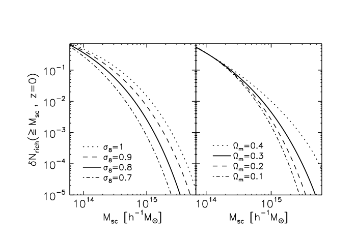
Using our analytic formula for the supercluster mass function constructed in section 2, we can evaluate $\delta N_{\rm rich}$ as a function of $z$. We first investigate the variation of $\delta N_{\rm rich}$ with the key cosmological parameters in the standard $\Lambda$CDM model. Figure 6 plots the relative abundance of the rich superclusters $\delta N_{\rm rich}$ at $z=0$ as a function of $M_{\rm sc}(\geq 10^{15}\,h^{-1}M_{\odot})$ for four different cases of the density parameter $\Omega_{m}$ (left panel) and for four different cases of the linear power spectrum amplitude $\sigma_{8}$ (right panel).

For the evaluation of the analytic supercluster mass function, the other cosmological parameters are set at the WMAP7 values (Komatsu et al., 2011) while the characteristic parameters of the supercluster mass function are consistently set at $\lambda_{1c}=1$ and $\lambda_{2c}=0.5$. As can be seen, the variations of $\sigma_{8}$ and $\Omega_{m}$ affect significantly the relative abundance of the rich superclusters $\delta N_{\rm rich}$ especially in the high mass section. As each of $\Omega_{m}$ and $\sigma_{8}$ increases, $\delta N_{\rm rich}$ drops less rapidly with $M_{\rm sc}$. This result is consistent with the picture that the cosmic web grows faster and the clusters merge more frequently in a universe where the initial density fluctuation has higher amplitude and dark matter are more dominant.

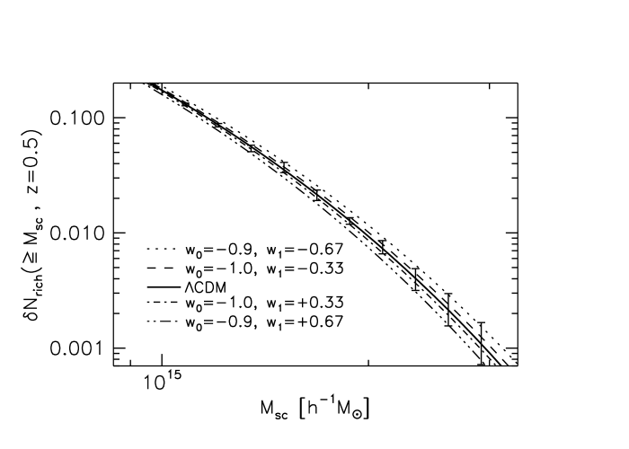
Assuming that our formula for the supercluster mass function, equation (1), also works in QCDM models (Quintessence+CDM) in which the Quintessence scalar field as a dynamical dark energy is responsible for the cosmic acceleration (e.g., Caldwell et al., 1998), we also perform a feasibility study on how well $\delta N_{\rm rich}$ can constrain the dark energy equation of state, $w$, defined as $w\equiv P_{Q}/\rho_{Q}$ where $P_{Q}$ and $\rho_{Q}$ represent the pressure and density of the Quintessence scalar field, respectively. For this test, we focus on a toy model in which the dark energy equation of state is given as $w(z)=w_{0}+w_{1}z/(1+z)^{2}$ where the two parameters, $w_{0}$ and $w_{1}$, have constant values (Chevallier & Polarski, 2001; Linder, 2003). For the evaluation of the supercluster mass function for this toy QCDM model, we use the approximate analytic formula for the QCDM linear growth factor given in Basilakos (2003) (see also Percival, 2005).

Figure 7 plots the relative abundance of the rich superclusters $\delta N_{\rm rich}$ at $z=0.5$ for five different cases of the dark energy equation of states. The Jackknife errors from the MICE simulations are also overlapped with our models to show explicitly how tight the constraints from the relative abundance of the rich superclusters would become if the same number of the superclusters were observed in the universe. As can be seen, $\delta N_{\rm rich}$ shows an appreciable change with $w(z)$ in the high-mass section ($M_{\rm sc}\geq 10^{15}\,h^{-1}M_{\odot}$). As the value of $w_{1}$ varies from $-0.67$ to $0.67$, the value of $\delta N_{\rm rich}$ decreases by a factor of two on the mass scale of $M_{\rm sc}=3\times 10^{15}\,h^{-1}M_{\odot}$, which indicates that the abundance of the rich superclusters at a given epoch must be useful to constrain the dark energy equation of state.

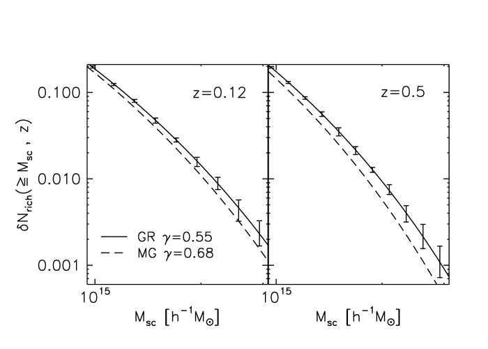
Finally, we also study how $\delta N_{\rm rich}$ changes in a toy modified gravity (MG) model in which the linear growth factor scales as a power law of the density parameter, $D(z)\propto\Omega_{m}^{\gamma}$ (e.g., see Linder, 2003, 2005). This toy MG model is distinguishable from the standard model (GR+$\Lambda$CDM) in the value of $\gamma$: In the former it is $\gamma=0.68$ while in the latter it is approximately $\gamma=0.55$ (Shapiro et al., 2010). Assuming that our formula for the supercluster mass function also works in this toy MG model, we evaluate $\delta N_{\rm rich}$, which is plotted in Figure 8 (dashed line). The standard (GR+$\Lambda$CDM with WMAP7 parameters) case is also plotted with the Jackknife errors for comparison (solid lines) at $z=0.12$ and $z=0.5$ in the left and right panels, respectively. The Jackknife errors at $z=0.12$ and $z=0.5$ are obtained from the CoDECS and MICE simulations, respectively. The difference in $\delta N_{\rm rich}$ between the two models at $M_{\rm sc}=3\times 10^{15}\,h^{-1}M_{\odot}$ reaches up to $50\%$ and $66\%$ at $z=0.12$ and $0.5$, respectively, which indicates that the relative abundance of the rich superclusters at a given epoch must be a useful indicator of modified gravity.

5 DISCUSSION AND CONCLUSION

In the framework of the EZL model constructed in our previous work (Lim & Lee, 2013), we have provided an efficient formula for the supercluster mass function with two characteristic parameters. The best merit of our formula is that its characteristic parameters are robust against variation of the background cosmology and independent of redshifts. Extrapolating its validity to non-standard cosmologies, we have suggested that the relative abundance of the rich superclusters at a given epoch should be powerful as a cosmological probe. This is the most accurate formula for the supercluster mass function that has ever been constructed, achieving a quantitative success in numerical tests.

Despite the fact that our formula for the supercluster mass function is not a physical one but a merely empirical one, the excellent agreements of the formula with the numerical results lead us to expect a wide application of the supercluster mass function to various fields. For example, as mentioned in Oguri et al. (2004), we expect it to be useful in quantifying how significant the effect of the presence of the warm hot intergalactic media on the superclusters (Myers et al., 2004; Zappacosta et al., 2005; Sadeh & Rephaeli, 2005). Our formula may also allow us to analytically estimate the late-time integrated Sachs-Wolfe (ISW) effect of superclusters (e.g., Granett et al., 2008, and references therein).

Before comparing our formula with the supercluster mass function from the real universe, however, we will have to undertake a couple of follow-up tasks. The first task is to examine whether or not our formula really works for non-standard cosmologies and investigate how its characteristic parameters change when the cosmological constant is replaced by the Quintessence scalar field and when there exists a fifth force generated by modified gravity. The second task is to account for the projection effect along the directions of the line-of-sight on the mass measurement of the superclusters. Since most of the superclusters have elongated shapes along the cosmic filaments (e.g., Einasto et al., 2011; Tempel et al., 2012), it would be harder to find the member clusters due to the projection effect if a supercluster happens to be elongated along the direction of the line-of-sight. We plan to conduct these follow-up works and to report the results elsewhere in the future.

Figure 1: Conditional probability, $P(M,M^{\prime})$ in equation (20), for four different cases of the characteristic parameters.

Figure 2: Comparison of the supercluster mass functions (solid line) with the numerical results from the Millennium simulations (dots) at three different redshifts. In each panel the errors represent the one standard deviation scatter among eight Jackknife resamples. The mass threshold for the supercluster membership, $M_{\rm c,th}$ is set at $10^{13}\,h^{-1}M_{\odot}$.

Figure 3: Same as Figure 2 but with the numerical results from the CoDECS simulations.

Figure 4: Same as Figure 2 but for the numerical results from the MICE simulations. The mass threshold, $M_{\rm c,th}$, for the supercluster membership is $3.4\times 10^{13}\,h^{-1}M_{\odot}$ from the MICE sample.

Figure 5: Same as Figures 2 and 3 but for the case that $M_{\rm c,th}=3.4\times 10^{13}\,h^{-1}M_{\odot}$, the same value used for the MICE sample, is adopted for the construction of the mass-limited cluster samples from the Millennium simulation (left panel) and from the CoDECS simulations (right panel).

Figure 6: Relative abundance of the rich superclusters at $z=0$ for four different cases of $\sigma_{8}$ (left panel) and for four different cases of $\Omega_{m}$ (right panel).

Figure 7: Relative abundance of the rich superclusters at $z=0.5$ for four different cases of the dark energy equation of state, $w(z)=w_{0}+w_{1}z/(1+z)^{2}$, assuming a toy QCDM model. The fiducial $\Lambda$CDM model (with $w_{0}=0,\ w_{1}=0$ and WMAP7 parameters) is also shown (solid line) for comparison. The errors are estimated as one standard deviation among $8$ Jackknife resamples from the MICE datasets.

Figure 8: Relative abundances of the rich superclusters for the case of the fiducial model (GR+$\Lambda$CDM with WMAP7 parameters) (solid line) and for the case of a toy model with modified gravity with $D(z)=\Omega^{0.68}_{m}$ (dashed line) at $z=0.12$ and $z=0.5$ in the left and right panel, respectively. The errors are estimated as one standard deviation scatter among $8$ Jackknife resamples from the CoDECS (left) and MICE (right) datasets.

Table 1: Simulation, linear box size, total number of dark matter particles, mass resolution, cosmological parameters and halo-finding algorithm.

Simulation	$L_{\rm box}$	$N_{\rm p}$	$M_{\rm p}$	$(\Omega_{m},\ \sigma_{8},\ n)$	Halo-Finder
	[$h^{-1}$Mpc]		[$10^{8}\,h^{-1}M_{\odot}$]
Millennium	$500$	$10^{10}$	$8.6$	$(0.25,\ 0.9,\ 1)$	FoF
CoDECS	$1000$	$2\times 1024^{3}$	$500.84$	$(0.271,\ 0.809,\ 0.966)$	FoF
MICE	$3072$	$2048^{3}$	$2300.42$	$(0.25,\ 0.8,\ 0.95)$	FoF

Table 2: Mass-limited sample, simulation, cluster mass threshold, total number of superclusters and mean supercluster mass at $z=0$.

simulation	$M_{\rm c,th}$	$N_{\rm tot}$	$\bar{M}_{\rm sc}$
	[$10^{13}h^{-1}M_{\odot}$]		[$10^{13}\,h^{-1}M_{\odot}$]
Millennium	$1.0$	$35422$	$5.7$
CoDECS	$1.0$	$412337$	$6.7$
MICE	$3.4$	$1851534$	$13.7$
Millennium	$3.4$	$9749$	$14.0$
CoDECS	$3.4$	$82016$	$12.6$

Table 3: Same as Table 2 but for $z=0.5$ ($z=0.44$ for CoDECS).

simulation	$M_{\rm c,th}$	$N_{\rm tot}$	$\bar{M}_{\rm sc}$
	[$10^{13}h^{-1}M_{\odot}$]		[$10^{13}\,h^{-1}M_{\odot}$]
Millennium	$1.0$	$26333$	$4.5$
CoDECS	$1.0$	$333739$	$5.5$
MICE	$3.4$	$1091086$	$11.3$

Table 4: Same as Table 2 but for $z=1$.

simulation	$M_{\rm c,th}$	$N_{\rm tot}$	$\bar{M}_{\rm sc}$
	[$10^{13}h^{-1}M_{\odot}$]		[$10^{13}\,h^{-1}M_{\odot}$]
Millennium	$1.0$	$17518$	$3.8$
CoDECS	$1.0$	$214386$	$4.4$
MICE	$3.4$	$494388$	$9.3$

References

- Araya-Melo et al. (2009) Araya-Melo, P. A., Reisenegger, A., Meza, A., et al. 2009, MNRAS, 399, 97
- Baldi (2012) Baldi, M. 2012, MNRAS, 422, 1028
- Bardeen et al. (1986) Bardeen, J. M., Bond, J. R., Kaiser, N., & Szalay, A. S. 1986, ApJ, 304, 15
- Basilakos (2003) Basilakos, S. 2003, ApJ, 590, 636
- Bode et al. (2009) Bode, P., Ostriker, J. P., & Vikhlinin, A. 2009, ApJ, 700, 989
- Buchdahl (1970) Buchdahl, H. A. 1970, MNRAS, 150, 1
- Busha et al. (2005) Busha, M. T., Evrard, A. E., Adams, F. C., & Wechsler, R. H. 2005, MNRAS, 363, L11
- Caldwell et al. (1998) Caldwell, R. R., Dave, R., & Steinhardt, P. J. 1998, Physical Review Letters, 80, 1582
- Chevallier & Polarski (2001) Chevallier, M. & Polarski, D. 2001, Int. J. Mod. Phys. D, 10, 213
- Clifton et al. (2012) Clifton, T., Ferreira, P. G., Padila, A., & Skordis, C. 2012, Physics Reports, 513, 1
- Coles et al. (1993) Coles, P., Melott, A. L., & Shandarin, S. F. 1993, MNRAS, 260, 765
- Crocce et al. (2010) Crocce, M., Fosalba, P., Castander, F. J., & Gaztañaga, E. 2010, MNRAS, 403, 1353
- Davis et al. (1985) Davis, M., Efstathiou, G., Frenk, C. S., & White, S. D. M. 1985, ApJ, 292, 371
- Desjacques (2008) Desjacques, V. 2008, MNRAS, 388, 638
- Desjacques & Smith (2008) Desjacques, V., & Smith, R. E. 2008, Phys. Rev. D, 78, 023527
- Doroshkevich (1970) Doroshkevich, A. G. 1970, Astrofizika, 6, 581
- Einasto et al. (2011) Einasto, M., Liivamägi, L. J., Tago, E., et al. 2011, A& A, 532, A5
- Granett et al. (2008) Granett, B. R., Neyrinck, M. C., & Szapudi, I. 2008, ApJ, 683, L99
- Jedamzik (1995) Jedamzik, K. 1995, ApJ, 448, 1
- Jones et al. (1993) Jones, M., et al. 1993, Nature, 365, 320
- Kasun & Evrard (2005) Kasun, S. F., & Evrard, A. E. 2005, ApJ, 629, 781
- Komatsu et al. (2011) Komatsu, E., Smith, K. M., Dunkley, J., et al. 2011, ApJS, 192, 18
- Lahav et al. (1991) Lahav, O., Lilje, P. B., Primack, J. R., & Rees, M. J., 1991, MNRAS, 251, 128
- Lee & Evrard (2007) Lee, J., & Evrard, A. E. 2007, ApJ, 657, 30
- Lewis et al. (2000) Lewis, A., Challinor, A., & Lasenby, A. 2000, ApJ, 538, 473
- Lim & Lee (2013) Lim, S., & Lee, J. 2013, JCAP, 1, 19
- Linder (2003) Linder, E. V. 2003, Phys.Rev.Lett, 90, 091301
- Linder (2005) Linder, E. V. 2005, Phys. Rev. D, 72, 043529
- Ludlow & Porciani (2011) Ludlow, A. D., & Porciani, C. 2011, arXiv:1107.5808
- Myers et al. (2004) Myers, A. D., Shanks, T., Outram, P. J., Frith, W. J., & Wolfendale, A. W. 2004, MNRAS, 347, L67
- Nagamine & Loeb (2003) Nagamine, K., & Loeb, A. 2003, New Astronomy, 8, 439
- Oguri et al. (2004) Oguri, M., Takahashi, K., Ichiki, K., & Ohno, H. 2004, arXiv:astro-ph/0410145
- Percival (2005) Percival, W. J. 2005, A& A, 819, 830
- Pillepich et al. (2010) Pillepich, A., Porciani, C., & Hahn, O. 2010, MNRAS, 402, 191
- Press & Schechter (1974) Press, W. H., & Schechter, P. 1974, ApJ, 187, 425
- Sadeh & Rephaeli (2005) Sadeh, S., & Rephaeli, Y. 2005, New Astronomy, 10, 560
- Shandarin & Zeldovich (1989) Shandarin, S. F., & Zeldovich, Y. B. 1989, Reviews of Modern Physics, 61, 185
- Shapiro et al. (2010) Shapiro, C., Dodelson, S., Hoyle, B., Samushia, L., & Flaugher, B. 2010, Phys. Rev. D, 82, 043520
- Shen et al. (2006) Shen, J., Abel, T., Mo, H. J., & Sheth, R. K. 2006, ApJ, 645, 783
- Sheth & Tormen (1999) Sheth, R. K., & Tormen, G. 1999, MNRAS, 308, 119
- Springel et al. (2005) Springel, V., White, S. D. M., Jenkins, A., et al. 2005, Nature, 435, 629
- Sunyaev & Zeldovich (1970) Sunyaev, R. A., & Zeldovich, Y. B. 1970, Comments on Astrophysics and Space Physics, 2, 66
- Sunyaev & Zeldovich (1972) Sunyaev, R. A., & Zeldovich, Y. B. 1972, Comments on Astrophysics and Space Physics, 4, 173
- Tempel et al. (2012) Tempel, E., Tago, E., & Liivamägi, L. J. 2012, A&A, 540, A106
- Tinker et al. (2008) Tinker, J. L., et al. 2008, ApJ, 688, 709
- Tully (1982) Tully, R. B. 1982, ApJ, 257, 389
- Wray et al. (2006) Wray, J. J., Bahcall, N. A., Bode, P., Boettiger, C., & Hopkins, P. F. 2006, ApJ, 652, 907
- Yan & Fan (2011) Yan, H., & Fan, Z. 2011, ApJ, 730, 33
- Zappacosta et al. (2005) Zappacosta, L., Maiolino, R., Mannucci, F., Gilli, R., & Schuecker, P. 2005, MNRAS, 357, 929
- Zel’dovich (1970) Zel’Dovich, Y. B. 1970, A& A, 5, 84