Rejoinder

10.1214/10-STS345

Rejoinder of Feature Matching in Time Series Modeling by Y. Xia and H. Tong

and

We would like to thank all the discussants for their wide-ranging comments. Before we respond to them individually in alphabetical order, we would like to address some general issues first. As we have said, we have chosen to describe our aim of matching the joint distribution of the observable data as feature matching, for want of a better name. We should have perhaps emphasized that we regard cycles, spectral singularities, and so on only as partial aspects of the joint distribution. They are useful, in practical applications, only in so far as they can provide partial measures of feature matching. We think Professor Hansen has understood our aim well in his introduction. We have sometimes, for brevity, called our general approach to achieving this aim the catch-all approach. We should stress the following point once more. The catch-all approach is not restricted to catch all first-order (conditional) moments or catch all second-order moments. We have used them in the paper primarily as illustrations of what the approach can deliver in modeling, beyond conventional methods based on the one-step-ahead prediction errors. Clearly, once the catch-all idea is accepted, we can equally well catch all $k$th-order (conditional or unconditional) moments, catch all marginal (conditional or unconditional) distributions, and so on. Moreover, the objective function $Q$ can also take on a form other than that of a mean squared type; for example, it can be of a likelihood type as stated in Section 2.1.

Professors Chan and Tsay have tried the catch-all approach on two real data sets, namely (i) the CREF stock fund and (ii) the monthly global temperature anomalies from 1880 to 2010. In each case, their implementation of the approach is exemplary. In data set (i), the catch-all approach has led to parameter estimates of the postulated $\operatorname{GARCH}(1,1)$ model that enable the model to “track the squared returns more closely” and “transit into the ensuing quiet period at a faster rate commensurate with the data.” We are sure that Chan and Tsay are aware of the fact that the larger is $\alpha$, the more responsive is the $\operatorname{GARCH}(1,1)$ model to volatility.

Chan and Tsay seem to be disappointed with their attempt with data set (ii). They have correctly noted the shapes of the eventual forecasting functions (eff) of the $\operatorname{ARIMA}(1,1,1)$ model and the $\operatorname{ARMA}(1,1)$-plus-trend model. Now, long-range forecasting invokes a low pass filter, which is approximately provided by the eff. Therefore, for an $\operatorname{ARIMA}(1,1,1)$ model, for sufficiently large $l$ and conditional on $Y_{s}$, $s\leq t$, $EY_{t+l}\approx K$, where $K$ is a constant. In such cases, $\phi\approx-\theta$, the well-known near cancelation of the AR operator and the MA operator. Similar arguments apply to an $\operatorname{ARMA}(1,1)$ model. It is clear in the setup of Chan and Tsay, as $m$ increases, long-range forecasts exert greater and ultimately overwhelming influence on the objective function, $S$.Thus, evidence of operator near cancelation with increasing $m$ is evidence of plausibility of the postulated model. This argument suggests that if Chan and Tsay had perhaps probed further with their Figure 2, they might be marginally more inclined toward the $\operatorname{ARMA}(1,1)$-plus-trend model. Of course, we must always be very cautious if we entertain any thought of extrapolating the trend into the future.

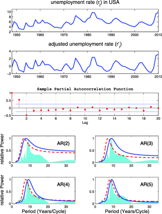
Taking up the challenge posed by Chan and Tsay relating to business cycles, we have considered the unemployment rate in the United States. The second panel of Figure 1 shows the rate after the removal of a moving mean. The partial autocorrelation function suggests strong $\operatorname{AR}(2)$ effect with a hint of higher order dependence. Figure 1 compares the spectral density functions of the $\operatorname{AR}$ model, from order 2 to 5, fitted respectively by the catch-all approach and the maximum likelihood approach. The former approach seems to show an overall better matching of the observed. The fundamental period of 9 years is clearly discernible and reasonably well captured by the $\operatorname{AR}(3)$, $\operatorname{AR}(4)$ and $\operatorname{AR}(5)$ models fitted by the catch-all approach. The possible existence of higher harmonics deserves further investigation, however.

Figure 1: The first panel is the unemployment rate ($r_{i}$) in the United States. The second panel adjusts it to $r_{i}^{\prime}=r_{i}-(r_{i-5}+r_{i-4}+\cdots+r_{i+5})/11$. Panel 3 is the plot of partial autocorrelation function with approximate 95% confidence interval. In each of panels 4–7, the edge of the shaded area is the power spectrum of time series $\{r_{i}^{\prime}\}$. The red dashed line and blue solid line are those of the models estimated by $\operatorname{APE}(1)$ and $\operatorname{APE}({<}T)$, respectively.

Professor Hansen has made numerous perceptive comments. We are much heartened by his endorsement of our most serious criticisms of what we now call the unreasonableness of one-step-ahead-prediction-error based methods. By paraphrasing Chan and Tsay, these methods have been used as if they were “one-size-fits-all” for far too long. Like the ancient practice of foot-binding among Chinese women, they are constrictive and painful. We advocate foot-unbinding. Needless to say, we are not so naive as to overlook the initial pains in unbinding or so arrogant as to rule out the possibility of other ways to unbind.

We are also very grateful to Professor Hansen for furthering the spirit of our Theorem C. We are in broad agreement with his analysis. Our only quibble is with his reference (also raised by Professor Ionides) to efficiency. For a wrong model, the conventional notion of efficiency can be misleading. White (1982) is relevant. We agree with Professor Hansen that there are many troubling problems with measurement errors. Our own contributions are quite modest in comparison with the enormity of the problems. Even rounding the data can be very troublesome already. See, for example, Zhang, Liu and Bai (2009).

Professor Ionides is clearly a faithful adherent to the maximum likelihood doctrine. Box’s dictum tells us that all models are wrong. Although some of them might be useful, they are still wrong. (Our paper does not address model selection. We shall return to this point later.) For a wrong model, what do we mean by efficiency or consistency? How would we assess likelihood ratios or AIC? Conventional treatments are characteristically invalid in their original forms. For example, we have highlighted the loss of a minimal set of sufficient statistics in Section 1.2. Professor Ionides must accept that the loss has by and large rendered the maximum likelihood type of estimation impotent. Next, for a wrong model, the Hessian matrix will typically have an expectation not equal to the negative of the variance of the score matrix. This clearly has implications on efficiency. As a third example, in the absence of a true parameter, the notion of consistency will have to be re-defined. It is precisely for this purpose that we have proposed the notion of a ($w$-dependent) optimal parameter. (By taking the infimum with respect to $w$, we can also define the notion of an optimal parameter.) Other examples abound. We would suggest that it is high time that we unbound our feet.

Figure 2: Results of fitting the new model to Nicholson’s blowflies data. In the first two panels, the dashed lines are for the observed population; the solid lines are for realizations from models fitted by $\operatorname{APE}({\leq}1$) and $\operatorname{APE}({\leq}T$), respectively. The dashed lines in panels 3 and 4 are the periodograms of the observed data, and the solid lines are those of the models fitted by $\operatorname{APE}({\leq}1$) and $\operatorname{APE}({\leq}T$), respectively.

The critical re-examination by Professor Ionides of the substantive model that we have fitted to the blowfly data has revealed an interesting situation. While the catch-all approach produces parameter estimates that lead to a good statistical fit to the observed data, they are not scientifically plausible. On the other hand, while the maximum likelihood type estimates of the parameters of the same model lead to a poor statistical fit, they are scientifically plausible. We take the view that this apparent dichotomy suggests that even a substantive model is not sacrosanct; an ideal model should be, at least, satisfactory both statistically and scientifically. Indeed, prompted by the alternative substantive model suggested by Ionides, we have considered the following simple equivalent of his model by merging his unobservable $R_{t}$ and $S_{t}$ into the available bi-daily data:

$$x_{t}=\operatorname{Poisson}\bigl{(}cx_{t-\tau}\exp(-x_{t-\tau}/N_{0})+\nu x_{t-1}\bigr{)}.$$

The maximum likelihood estimates (with Poisson distribution) are

$$c=8.49,\quad N_{0}=528.23,\quad\nu=0.77$$

and the catch-all estimates (with the objective function based on all-step-ahead predictors) are

$$c=8.82,\quad N_{0}=604.98,\quad\nu=0.67.$$

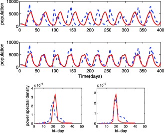
Both sets of parameter estimates are broadly consistent with those obtained by Professor Ionides for his new model ($c=2\times 3.28,N_{0}=680,\nu=\exp(-2\delta)=0.7247$), and lead to scientifically plausible models ($c$ being the reproducing rate). On the other hand, Figure 2 shows that the catch-all approach gives a good fit to the observed periodicity but the maximum likelihood approach does not. Similar remark applies to the fitted period as a function of time to maturity (not shown as the results are similar to panels 5 and 6 of Figure 8 in the paper). It is unfortunate that results of the statistical goodness of fit of his alternative model are not available.

Professor Yao is clearly alert and has noted our fleeting reference to the important issue of model selection among wrong models. He has given some valuable thoughts on the issue, for which we are most grateful. We suspect that he will also agree with us that the general problem is much deeper. The reference to Konishi and Kitagawa (1996) is apt. As for his quibble, if he can throw us a more catchy line than catch-all, we would be happy to catch it. Perhaps, “foot-unbinding” might be a better name in reflecting the philosophy of our approach.

References

- Konishi and Kitagawa (1996) {barticle}[mr] \bauthor\bsnmKonishi, \bfnmS.\binitsS. and \bauthor\bsnmKitagawa, \bfnmG.\binitsG. (\byear1996). \btitleGeneralised information criteria in model selection. \bjournalBiometrika \bvolume83 \bpages875–890. \endbibitem
- White (1982) {barticle}[mr] \bauthor\bsnmWhite, \bfnmHalbert\binitsH. (\byear1982). \btitleMaximum likelihood estimation of misspecified models. \bjournalEconometrica \bvolume50 \bpages1–25. \biddoi=10.2307/1912526, issn=0012-9682, mr=0640163 \endbibitem
- Zhang, Liu and Bai (2009) {barticle}[auto:STB—2011-03-03—12:04:44] \bauthor\bsnmZhang, \bfnmB.\binitsB., \bauthor\bsnmLiu, \bfnmT.\binitsT. and \bauthor\bsnmBai, \bfnmZ. D.\binitsZ. D. (\byear2009). \btitleAnalysis of rounded data from dependent sequences. \bjournalAnn. Inst. Statist. Math. \bvolume62 \bpages1143–1173. \endbibitem