Coarse-graining strategies in polymer solutions
Abstract
We review a coarse-graining strategy (multiblob approach) for polymer solutions in which groups of monomers are mapped onto a single atom (a blob) and effective blob-blob interactions are obtained by requiring the coarse-grained model to reproduce some coarse-grained features of the zero-density isolated-chain structure. By tuning the level of coarse graining, i.e. the number of monomers to be mapped onto a single blob, the model should be adequate to explore the semidilute regime above the collapse transition, since in this case the monomer density is very small if chains are long enough. The implementation of these ideas has been previously based on a transferability hypothesis, which was not completely tested against full-monomer results (Pierleoni et al., J. Chem. Phys., 2007, 127, 171102). We study different models proposed in the past and we compare their predictions to full-monomer results for the chain structure and the thermodynamics in the range of polymer volume fractions between 0 and 8. We find that the transferability assumption has a limited predictive power if a thermodynamically consistent model is required. We introduce a new tetramer model parametrized in such a way to reproduce not only zero-density intramolecular and intermolecular two-body probabilities, but also some intramolecular three-body and four-body distributions. We find that such a model correctly predicts three-chain effects, the structure and the thermodynamics up to , a range considerably larger than that obtained with previous simpler models using zero-density potentials. Our results show the correctness of the ideas behind the multiblob approach but also that more work is needed to understand how to develop models with more effective monomers which would allow us to explore the semidilute regime at larger chain volume fractions.
1 Introduction
Polymer solutions show a wide variety of behaviors, depending on chain length, density, and temperature.[1, 2, 3, 4] In the dilute regime the isolated chain radius of gyration is the relevant length scale and the properties of the solution can be described in terms of single-chain properties and of the solvent-quality parameter. The radius of gyration scales as , where is the monomer characteristic length (Kuhn segment), which depends on chemical details and temperature, is the number of monomers per chain, and is a universal exponent. In the good-solvent regime[5] , while (with logarithmic corrections [3, 4]) for -solvents. The semidilute regime is entered when chains start to overlap, but still the monomer density is small. If is the polymer concentration — is the number of chains and the volume of the system under consideration — and is the monomer concentration, the semidilute regime is characterized by (or equivalently by , where is the polymer volume fraction) and , where is the overlap concentration. Note that . Hence, when increasing , increasingly longer polymer chains are needed to ensure the semidilute condition . If is not small, one enters the concentrated or melt regime.
From this discussion it appears that very long polymers are necessary to obtain a genuine semidilute regime over several orders of magnitude in chain density. For this reason, simulations of semidilute solutions of linear chains, even at the level of generic lattice or bead-spring models with implicit solvent, are quite expensive and have been limited to not too long chains and not too high densities. [6, 7, 8, 9, 10, 11] Moreover, in many complex situations, polymers only constitute one species in the solution, making full-monomer simulations even more difficult. In these cases a modelling at length scales of the order of the polymer size is often sufficient to provide the relevant thermodynamic and structural informations on the solution. For instance, to determine the phase behavior of polymer-colloid mixtures in the colloid regime, [12, 13, 14, 15] a detailed microscopic model of the polymers is not necessary. It is enough to use coarse-grained models which retain the essential thermodynamic (long-wavelength) behavior of the polymer solution.[16] Other examples are block copolymers for which the self-assembling of the chains in supramolecular aggregates of various shapes and sizes is ubiquitous. The description of the physical behavior of the self-assembled phases only requires a modelling at the mesoscopic level rather than at the microscopic (monomer) level. [17, 18, 19, 20] This is the realm of self-consistent field-theoretical methods which have proved to be very effective to describe the physics of concentrated solutions and melts of homopolymers and block-copolymer blends. [21, 7]
Coarse-grained models for soft condensed matter systems have received much attention in the last two decades.[22] In the simplest approach one maps polymer chains onto point particles interacting by means of the pairwise potential of mean force between the centers of mass of two isolated polymers. [23, 22] This potential is of the order of at full overlap,[24, 25] has a limited range of the order of and is very well represented by a linear combination of few Gaussian functions. [8, 11] Such a model is however limited to the dilute regime , in which many-body interactions[26] can be neglected. This limitation was overcome ten years ago in a seminal work,[27, 8] which eliminated the complexity of the many-body interactions by introducing a density-dependent pair potential, which is unique according to Henderson theorem [28] and reduces to the potential of mean force in the limit of zero density.
This work has paved the way to the use of soft effective particles to represent polymer coils in complex situations such as in modelling colloid-polymer mixtures.[16] However, density-dependent potentials are difficult to handle. Care is needed to derive the correct thermodynamics [29, 30, 31] and to compute free energies and phase diagrams.[22] Also their use in non-homogeneous situations is cumbersome since the interaction should depend on the local density which is not known beforehands and some kind of self-consistent procedure should be developed. Furthermore, representing polymers as soft spherically symmetric particles is not always appropriate. For instance, in studying polymers adsorbed on surfaces, like polymer brushes or polymer-coated colloids, it is clear that the anchorage to the surface breaks the rotational symmetry of the chains, an effect that must be taken into account in any accurate coarse-grained model. A further example is in modelling solutions of A-B block copolymers which cannot be represented as soft particles interacting by a spherically symmetric pair potential. [17, 18, 19, 20]
In principle those limitations can be overcome by switching to a model at a lower level of coarse graining, i.e. by mapping a long linear polymer to a short linear chain of soft effective monomers (called “blobs” in the following). Such model retains some internal degrees of freedom, which allow more flexibility in chain geometry as necessary, for instance, in anisotropic systems. Moreover, in the semidilute regime, this model is expected to allow the use of density-independent blob-blob interactions, since the local density of the blobs can always be kept small by increasing the number of blobs per chain. Indeed, if chains of monomers are partitioned in effective blobs of monomers each, the local concentration of the blobs is . The blob overlap concentration is given by , where is the radius of gyration of the blob. If we assume that , where is the Kuhn length that appears in the scaling of the radius of gyration (this relation, though not exact, is a very good approximation), we obtain
| (1) |
Hence, for any polymer volume fraction , since above the collapsed phase, one can choose so that , i.e., so that blobs do not overlap. In this regime, the size of each blob is approximately density independent, hence each blob can be replaced by an effective single atom of fixed size in a coarse-grained representation. Moreover, one expects the many-body interactions among blobs of different chains to be negligible. Hence, the parametrization of the intermolecular interactions among the chains in terms of zero-density pair potentials should be reasonably accurate. Conversely, one can use the blob model with zero-density intermolecular pair potentials up to . For larger concentrations many-chain intermolecular interactions come into play.
The main problem in this approach is how to obtain the intramolecular interactions, i.e., the potentials among the blobs of the same chain. The problem is trivial for a dumbbell model (), where the blob-blob interaction is just the potential of mean force, but becomes increasingly difficult when increasing the number of blobs per chain. Indeed, the intramolecular effective interaction, which is simply minus the logarithm of the joint distribution of the blob positions, is inherently a many-body interaction, which cannot be represented as a hierarchy of two-body, three-body, etc. terms, at variance with what happens for the intermolecular potentials. In that case the small-density expansion gives the pair potential at lowest order, the three-body potential at next-to-leading order, and so on. Therefore, approximations must be introduced in trying to reproduce some features of the underlying full-monomer system.
As a first attempt in this direction, Pierleoni et al. [32] introduced a multiblob model, referred to as model M1 in the following, for homopolymers in good-solvent conditions. They started from the intramolecular and intermolecular potentials appropriate for dumbbells (a two-blob molecule), a problem that can be solved as explained in Addison et al.[33] The potentials for chains with more blobs were then obtained from the dumbbell potentials using a transferability hypothesis. This model has the correct scaling behavior for good-solvent polymers in dilute and semidilute solutions, [32] including the excluded-volume screening at large length scales with density. However, its prediction for the EOS of the solution is incorrect,[34] shading serious doubts on the correctness of the transferability assumption for the potentials. A modified model, referred to as model M2 in the following, was also introduced.[34] In this model, for each number of blobs, the parameters of the potential are tuned to match full-monomer results for the EOS. Although successful in reproducing the thermodynamics, model M2 is inherently different from M1 in that full-monomer results at finite density are needed to tune the model parameters, which is an evident limitation of this approach in more complex situations.
In this paper, beside comparing in detail results for models M1 and M2 to full-monomer predictions in a wide range of polymer concentrations in the semidilute regime, we introduce a new coarse-grained model for semidilute solutions. In this model we map a single chain on a tetramer, i.e., a chain of four blobs, in such a way to reproduce all two-body, and some three-body and four-body distributions of an isolated good-solvent polymer at the full monomer level. In order to accomplish this program we use bonding, bending and torsional angle potentials, plus additional 1-3 and 1-4 central potentials which we obtain with the Iterative Boltzmann Inversion (IBI) procedure. [35, 36, 37] Furthermore, a single intermolecular pair potential between blobs of different tetramers is obtained in such a way to reproduce the center-of-mass radial distribution function between two isolated chains at the full-monomer level. This model provides correct results for the EOS up to reduced densities , a considerably larger range of densities with respect to simpler models. The tetramer model presented here is a first successful attempt to realize the multiblob program: building a multiblob coarse-grained model based on zero-density potentials which is able to provide the correct single-chain structure and EOS at finite density.
Our approach is very close to the coarse-graining procedure applied by Fritz et al.[38] to polystyrene. Similar methods were also used for coarse-grained simulations of typical benchmark chains like polycarbonates and polystyrene in a melt, [39, 40] although in these works the potentials were fixed by requiring the coarse-grained model to reproduce structural properties at fixed pressure and temperature — hence potentials also depend on thermodynamic variables, as is the case for the density-dependent potentials.[27, 8] In some coarse-graining procedures also thermodynamic information was taken into account to fix the potentials, see, e.g., Rossi et al.[41] and references therein. We should also mention the approach of Vettorel et al. [42], which extends previous work on a single-blob model.[43] In this multiblob model each blob carries internal degrees of freedom, to account for the density profile of the underlying full-monomer subchains. However, the interactions are not derived ab initio in the coarse-graining procedure, but are obtained by using phenomenological arguments. Finally, we mention the work of Clark et al. [44] which applies integral-equation methods to a coarse-grained model appropriate for polymer melts.
The paper is organized as follows. In section 2 we present the general formalism behind any coarse-graining procedure and we report our specific methodology to derive the tetramer model. In section 3 we compare the structure and the thermodynamic behavior predicted by the tetramer model with those (referred to as full-monomer results in the following) obtained by using lattice polymer models with a large number of monomers () — hence appropriate to obtain the universal, scaling behavior — both at zero and at finite density in the semidilute regime. In section 4 we report results for the coarse-grained models M1 and M2 and compare them with the tetramer and the full-monomer data. Finally, we collect our conclusions and perspectives in the last section. In the appendix we give universal predictions for the blob radius of gyration, an important quantity to obtain a meaningful comparison between any coarse-grained model and the underlying full-monomer model.
2 The blob model
In order to obtain the coarse-grained blob model (CGBM), one works in the zero-density limit and determines in successive steps the intramolecular potentials, the two-body intermolecular potentials, then, at least in principle, the three-body, four-body, etc. intermolecular potentials. In an exact mapping all -body intermolecular interactions should be considered. However, as discussed in the introduction, higher-order intermolecular interactions can be neglected if one only considers small densities , where increases (for a given level of approximation) with the number of blobs.
2.1 The blob representation of the polymer
In the multiblob approach, the basic object is the “blob”, which is a subchain of the polymer. Suppose we wish to partition a polymeric chain of monomers into blobs of monomers each. If the monomer positions are given by , one first defines the blob positions as the centers of mass of the subchains of monomers, i.e.
| (2) |
For the new coarse-grained chain one defines several standard quantities. First, one defines its radius of gyration
| (3) |
Such a quantity is always smaller than , since
| (4) |
where is the radius of gyration of -th blob:
| (5) |
The ratios and of their averages 111Note that here we use the same notation for the squared radius of gyration of a single-chain configuration and for its statistical average over all chain conformations. When we will need to distinguish between the two quantities, the average squared radius of gyration will be indicated as . over the polymer configurations are universal, hence independent of the nature of the underlying polymer model as long as is large enough. The average of the blob squared radius of gyration defined by scales quite simply with in the zero-density limit. As discussed in A, for all we have quite precisely
| (6) |
an expression we will use extensively in the present work (here and in the following we will use a hat to indicate zero-density quantities).
Beside the radius of gyration, we can consider the bond-length distributions (all blob distributions depend on the number of blobs, which is implicit in the notation)
| (7) |
where is the statistical average over all chain conformations, which satisfy the normalization conditions
| (8) |
They depend on the chosen length scale. As it is standard in renormalization-group analyses of polymer behavior, the relevant quantities are the adimensional combinations . For they converge to universal, hence model-independent, functions with , which are normalized as
| (9) |
Note that, as usual, scaling functions depend only on the adimensional combination .
In this paper we will also consider the adimensional intramolecular distribution function
| (10) |
For large , converges to a universal function , , which is related to the bond-distribution functions defined above by
| (11) |
Note that the the ratio is simply related to the second moment of [in the scaling limit to that of ]. For we have
| (12) |
Beside two-site distributions, one can define three-site correlation functions
| (13) |
— the corresponding adimensional combinations converge to universal functions of and — and, analogously, four-site, five-site, etc. correlations.
As a check of the quality of our results we shall often consider the distribution of . More precisely, for each polymer configuration we consider the corresponding radius and the adimensional ratio , where is the average of the squared radius of gyration over the polymer configurations. The corresponding distribution
| (14) |
is universal in the large- limit. Note that this distribution function cannot be written in terms of the bond-length distributions, but is instead a particular -blob correlation since depends on the positions of all blobs.
2.2 The coarse-grained model
In the CGBM the basic object is a polyatomic molecule with atoms located in . All length scales are expressed in terms of , hence potentials and distribution functions depend on the adimensional combination . The intramolecular potentials are determined by requiring all adimensional distributions to be identical in the polymer model and in the CGBM at zero density. For instance, we require
| (15) |
where is the average over all single-chain CGBM configurations and are the universal functions defined above, which are computed in the polymer model.
In principle, the determination of the intramolecular potential is straightforward. First, one determines the -body blob distribution in the polymer model at zero density:
| (16) |
where the average is over all single-polymer conformations. The adimensional combination converges for to a universal distribution:
| (17) |
where . The CGBM intermolecular potential is then
| (18) |
where . By definition, this choice ensures that the distribution of the atoms in the CGBM is identical to the distribution of the blobs in the polymer model. Hence the intramolecular structure is exactly reproduced. Note that potential (18) is an intrinsically -body interaction and thus there is no natural method to represent it as a sum of two-body, three-body, etc., terms. Because of the universality of the function , the potential is independent of the polymer model and is valid for any polymeric system under good-solvent conditions.
The radius of gyration of the CGBM molecule differs from the polymer radius of gyration but agrees instead with . It is important to take this difference into account when comparing finite-density results. For polymers, the behavior is universal once densities are expressed in terms of the polymer volume fraction
| (19) |
where is the number of polymers contained in the volume . Full-monomer results should be compared with results obtained in the CGBM at volume fractions
| (20) |
where is the number of CGBM molecules. Note that and not appears in the definition of . Since converges to 1 as increases, for large, say , this conceptual difference is not relevant in practice. In our case, instead, since we consider , it is crucial to use the correct definition, that is the quantity .
Once the intramolecular potentials are determined, one must determine the intermolecular potentials, which must be such to reproduce the potentials of mean force in the polymer model. Note that, in order to have an exact mapping of the polymer model onto the CGBM, not only should pair potentials be considered, but also three-body, four-body, etc. interactions should be included.[26, 11] However, as we already discussed in the introduction, as increases, these many-body interaction potentials are expected to become smaller, so that the CGBM with only pair potentials should be accurate in a density interval which widens with increasing .
2.3 Determination of the four-blob CGBM intramolecular potentials
In order to have an exact mapping of the polymeric system onto the -blob CGBM, one should consider an -body intramolecular potential, which, for , can be expressed in terms of scalar combinations of the positions of the blobs because of rotational and translational invariance. The complexity increases rapidly with and for this reason we decided to consider the case , which allows us to limit the number of approximations needed and, at the same time, allows us to go beyond the dilute regime up to -3. However, even for as small as 4, an exact determination of the intramolecular potential requires considering a function of 6 independent variables, which is far too complex in practice.
Thus we have used a limited set of interactions. The intramolecular interactions have been modelled by introducing six different potentials, each of them depending on a single scalar variable. This choice is arbitrary, but, as we will show in the following, it is particularly convenient and works quite well. First, we consider a set of bonding pair potentials: atoms and of the tetramer interact with a pair potential with . Because of symmetry we have and , so that there are only four independent potentials to be determined. Then, we consider a bending-angle potential and a torsion-angle potential , where and are defined as
| (21) | |||
| (22) |
with . Note that in the tetramer there are two bending angles, which are equivalent by symmetry, and a single torsion angle. This particular form of the potential set is inspired by the usual modelling of bonded interactions in macromolecules. However, in that context one only considers a bonding potential between atoms which are first neighbors along the chain, a bending and a torsional term. Instead, our parametrization includes interactions between atoms that are not neighbors along the chain, thereby taking into account to some extent cross-correlations among different degrees of freedom. We note that the bending potential and the torsion potential involve three and four atoms, respectively, and thus allow us to introduce some of the three-body and four-body interactions present in the exact parametrization.
Since we are using a limited set of interactions, not all distributions of the internal degrees of freedom can be exactly reproduced by the CGBM. We must therefore choose the distributions which we wish to be identical in the polymer and in the CGBM case. Given our choice of interaction potentials, it is natural to use the adimensional bond-length distributions and the distributions of the bending and torsion angle [in the blob representation of the polymer model, these angles are defined by replacing with in Eqs. (21) and (22)], which are particular three-body and four-body correlation functions. If we indicate collectively the six potentials to be determined with , the (adimensional) distributions of the variables with in the CGBM and with in the full-monomer case, the potentials should be such that . The universal (i.e., model-independent) distributions in the polymer case have been determined by performing simulations of self-avoiding walks on a cubic lattice. To detect scaling corrections, we consider chains of length , 4100 (the corresponding blobs have monomers, respectively). The (adimensional) distributions obtained in the two cases agree within errors, indicating the absence of finite-length effects.
We determine the potentials of the CGBM by using the Iterative Boltzmann Inversion (IBI) scheme. [35, 36, 37] In this approach the effective interactions which reproduce the target structural quantities are determined iteratively. The potentials of mean force of the corresponding full-monomer distribution, , have been chosen as initial guesses for all interactions except for . For we have assumed a simple Gaussian potential: we use a Gaussian approximation of the potential of mean force between two polymer centers of mass, rescaling the width of the Gaussian with the ratio of the radii of gyration of the blob and of the entire chain.
 |
 |
|
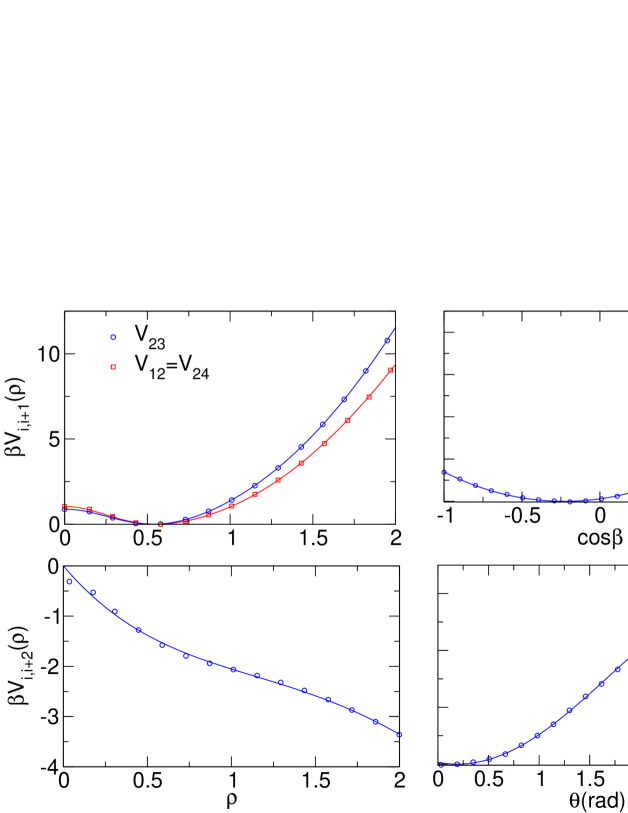 |
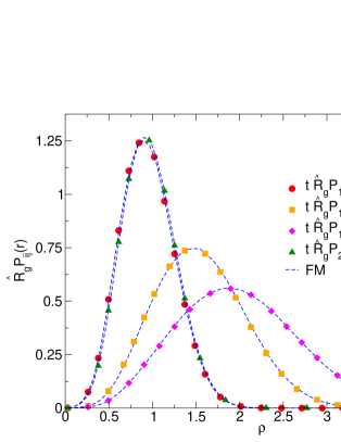
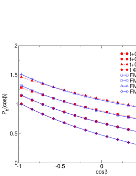
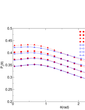
At the end of the optimization procedure, the bond and angle distributions are reproduced quite precisely, see figures 1 and 2. The potentials obtained are reported in figure 3. The pair potentials and are very similar, indicating that end effects are not very important. They have a minimum for and are very soft at the origin: -1.0). For they increase quite rapidly and for they approximately behave as () and (). The potential between next-nearest neighbors is continuously decreasing and hence it penalizes configurations in which the two atoms are close. Finally, appears to be irrelevant for . As for the bending-angle potential, it penalizes configurations with , while it is essentially flat for : the potential has a minimum for and . Finally, the torsion potential turns out to be quite flat: it increases with and changes only by , going from to .
The results for the potentials are quite interesting since they indicate the presence of an effective hierarchy among the different contributions. The pair potentials between neighbors are the most important. For instance, for typical configurations, say, for , see figure 1, the potentials and vary significantly, by 4-5. Instead, for typical distances , the potential varies much less, approximately by 2, while in the typical interval , varies only by 0.03. Clearly, the relevance of the interactions decreases as the chemical distance between the atoms increases, even though interactions between distant atoms can never be neglected, otherwise one would model a random-walk chain and not a polymer under good-solvent conditions.
The bending-angle potential varies at most by and is thus less relevant than the bonding potentials, while the torsion potential only provides a small correction. This seems to indicate that the relevance of the interactions decreases with the number of atoms involved, so that, when the number of atoms increases, one can safely neglect higher-body interactions.
It is important to stress that the pair potentials and are somewhat different from the potentials one would obtain by using the transferability hypothesis as suggested by Pierleoni et al.[32] If we use Eq. (6) to relate to , we would obtain a transferability potential (see the expression reported in the caption of figure 1 of Pierleoni et al.[32])
| (23) |
where . The minimum of this potential occurs for , to be compared with of and . Overlaps are more suppressed since (for our potentials we find -). Morever, the potential increases much less than or as increases. For instance, for , a value which occurs quite frequently, see figure 1, we have , while , .
2.4 Determination of the CGBM intermolecular potentials
As for the intermolecular potentials, we have made some drastic simplifications. First, we do not consider -body interaction terms, which, as we already mentioned, are important only for densities . Then, we consider a single intermolecular pair potential : the atoms interact with the same potential, irrespective of their positions along the chains. Such a potential has been obtained by requiring the CGBM to reproduce the center-of-mass intermolecular distribution function. Indeed, define in the polymer model
| (24) |
where indicates the average over two polymers, the centers of mass of which are in the origin and in , respectively, and is the intermolecular energy. In the scaling limit , converges to a universal function , . The pair potential has been determined so that
| (25) |
where is the corresponding distribution function in the CGBM. Note that the second virial coefficient is related to by
| (26) |
Hence, equality (25) guarantees that the adimensional combination , hence the thermodynamics in the small-density limit, agrees in the CGBM and in the polymer model.
The potential has been parametrized as
| (27) |
in terms of two unknown parameters and . They have been determined following the approach of Akkermans et al.[45, 46] Requiring the model to reproduce at best the polymer scaling function , we obtain the optimal values and . For these parameter values the model with potential (27) has an intermolecular pair distribution function which agrees quite precisely with the corresponding polymer quantity, see figure 4. The result depends on the parametrization and we cannot exclude that a different parametrization with the same number of parameters gives results of better quality. Potential (27) differs only slightly from the intramolecular potential . Interactions between the atoms at the ends of the chain or between atoms that belong to different chains are quite similar. It is interesting to compare our result with that one would obtain by using the transferability hypothesis as suggested by Pierleoni et al.: [32] . The range of the potential is the same, but the potential we obtain is somewhat softer.
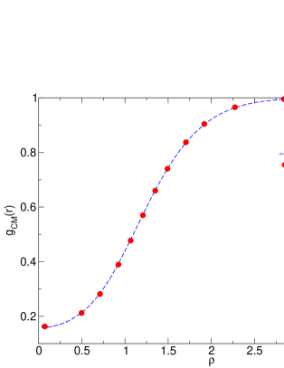 |
3 Comparison of CGBM and polymer results
In order to understand how well the tetramer model reproduces the polymer behavior we have performed extensive simulations of the tetramer and of a polymer model at zero density and at volume fractions , 4.36, 8.72. Since CGBM and polymer results should be compared taking , see (19) and (20), we drop the suffix and thus also refers to . At finite density polymers have been modelled by means of the Domb-Joyce (DJ) model with , a value which is close to the optimal one for which no leading scaling corrections are present (see Caracciolo et al.[47] for details on the model). It allows us to determine precisely the universal, model-independent scaling functions by using chains of moderate length. We consider walks of length and , verifying the practical absence of scaling corrections. As in previous work[48], we considered different box sizes, finding negligible size effects when the number of chains in the box exceeds 100. Simulations have been performed using the algorithm described in Pelissetto.[48]
3.1 Zero-density
By construction, the tetramer CGBM reproduces the bond-length distributions. As we have already remarked in Sec. 2.1, see (11) and (12), the ratio can be expressed in terms of these distributions, hence this ratio should assume the same value in the tetramer and in the polymer case. Numerically, we find for the tetramer and for the polymer case. The difference is approximately 0.1%, which shows how accurate the intramolecular potentials we determined are. Moreover, not only agrees, but also its distribution (14) is the same for polymers and tetramers, see figure 5a). This is a nontrivial check, since this distribution is not directly related to the bond-length distributions, nor to those of the bending and torsion angles. Clearly, the tetramer models correctly the shape and size of a polymer at zero density.
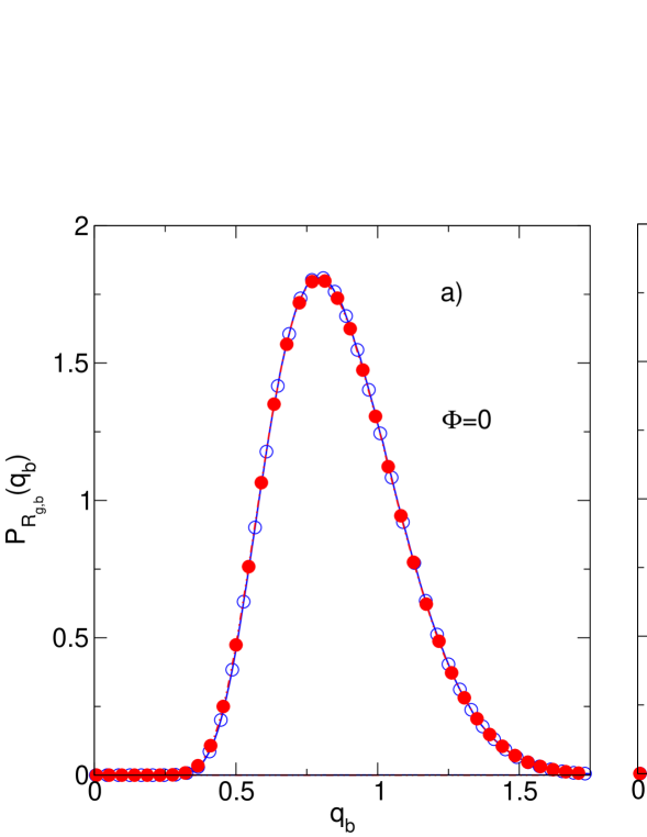 |
Since we have matched the center-of-mass distribution function to determine the intermolecular potential, the tetramer CGBM should give the correct second virial coefficient. If we expand the compressibility factor as
| (28) |
the quantity is universal. An accurate estimate is [47] . For the tetramer we obtain . The difference is approximatey 1.8% and is representative of the level of precision with which the tetramer model reproduces the center-of-mass distribution function. Much more interesting is the comparison of the third virial coefficient, since it provides an indication of the accuracy with which the tetramer model reproduces the polymer thermodynamics in the dilute regime and also of the importance of the neglected three-body forces. The universal combination was computed by Caracciolo et al.[47] finding .
In order to determine , two contributions had to be computed. One contribution is the standard one, the only present in monoatomic fluids and in fluids of rigid molecules, , while the second one is a flexibility contribution (it corresponds to in the notations of Caracciolo et al.[47]). The combination as well as the two contributions and are universal, hence it makes sense to compare them with the tetramer corresponding results. We obtain
| (29) |
The tetramer reproduces quite reasonably the third virial coefficient, the difference being approximately 2%. Note that much of the discrepancy is due to : the tetramer is more rigid than the polymer. It is interesting to compare these results with those obtained by using the single-blob model in which polymers are represented by monoatomic molecules interacting by means of density-independent potentials. 222If we were using density-dependent potentials, the thermodynamics, hence all virial coefficients, would be exactly reproduced. However, here we only consider models with density-independent potentials, hence the only meaningful comparison is with the single-blob model in which the interactions are density independent. If we use the accurate pair potential of Pelissetto et al.[11] we obtain (of course here ) which deviates by 20% from the polymer result. Hence, the tetramer model represents a significant improvement for the thermodynamics.
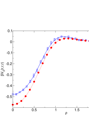 |
As a further check we compute the effective three-body potential of mean force defined by [26, 11]
| (30) |
here is the intermolecular potential energy between tetramers and and the average is over triplets of tetramers such that , where is the position of the center of mass of tetramer .
We computed for equilateral triangular configurations such that . The result is reported in figure 6 and compared with the analogous quantity computed in full-monomer simulations. At variance with the single-blob model for which , the tetramer model reproduces the polymer quite reasonably: differences — the tetramer potential is slightly more attractive — are observed for , but they are only significant for , i.e., when the tetramers are very close. This is consistent with the analysis of the third virial coefficient: in the dilute limit three-body interactions are correctly reproduced by the tetramer model, without the need of introducing a three-body potential among tetramer atoms.
3.2 Semidilute regime
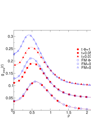 |
As we have discussed in the introduction, the tetramer model is expected to reproduce the full-monomer results up to , representing a significant improvement with respect to the single-blob model which shows large deviations already for . To check this expected behavior we compare tetramer and full-monomer simulations at , 4.36, and 8.72.
Let us begin with the structural properties. In figure 7 we report the adimensional intramolecular distribution function . For the agreement between the tetramer and the full monomer results is excellent. However, as increases, deviations are observed for . For the tetramer is more swollen than the polymer: the probability for two blobs to be at a given distance is significantly smaller in the tetramer than in the full-monomer chain. These results are further confirmed by the results for the radius of gyration. For the tetramer we have
| (31) |
to be compared with the full-monomer results
| (32) |
For the agreement is very good, consistently with the results reported in figure 7. As increases, however, the tetramer is more rigid than the polymer and is larger in the tetramer than in the polymer case. The same conclusions are reached by looking at the distribution of , see figure 5. For the agreement is excellent, while for the tetramer distribution is slightly shifted towards larger values of .
It is also interesting to compare the results for the bending and torsion angles reported in figure 2. The distributions appear to have a tiny dependence on and to be reasonably reproduced by the tetramer for all values of . For instance, for the largest value of , , we have for polymers , , to be compared with 0.88 and 0.354, respectively, in the tetramer case.
| 0.054 | 1.07363(3) | 1.0725 |
| 0.135 | 1.18993(4) | 1.1871 |
| 0.27 | 1.39852(6) | 1.3929 |
| 0.54 | 1.8499(1) | 1.8536 |
| 1.09 | 2.9090(1) | 2.9589 |
| 2.18 | 5.2660(2) | 5.6342 |
| 4.35 | 10.2056(4) | 12.229 |
| 6.53 | 15.2279(1) | 20.019 |
| 8.72 | 20.2811(1) | 28.716 |
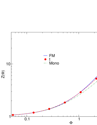 |
Let us now consider the thermodynamics. For this purpose we computed the compressibility factor for the tetramer using the molecular virial method [49, 50] ( is the number concentration). As is dimensionless, polymer and tetramer results at the same value of can be directly compared. Estimates are reported in Table 1. For the tetramer is very close to the polymer prediction: for it differs by 2% from the correct result. As increases, however, differences increase and the tetramer model underestimates the correct pressure. In figure 8 we compare for the tetramer with the corresponding expression for polymers.[48] At the scale of the figure, good agreement is observed up to . For larger densities, in the tetramer increases slower than in the polymer case. Indeed, while in polymers we expect for large , for the tetramer is expected to increase only linearly with (since the potential is soft, for the random-phase approximation should become exact [51]).
As can be seen from figure 8, the tetramer model is significantly better than the single-blob model,333 For the single-blob model we shall always use the accurate expression of the pair potential given in Pelissetto et al.[11] in which each polymer is represented by a single atom. At such a model gives , which underestimates by 8%, much more than the tetramer model (at this density the error on is 2%). The single-blob model gives a value for which differs from the polymer one by less than 2% only up to , i.e. up to densities which are a factor-of-three smaller than the corrisponding ones for the tetramer. This improvement confirms the scaling argument we presented in the introduction. As we explained in the introduction, the multiblob model should give the correct thermodynamics up to a polymer volume fraction which scales as . If we compare the tetramer model with the single-blob one, we thus expect the density range in which the model is predictive to increase by , which is indeed what we find.
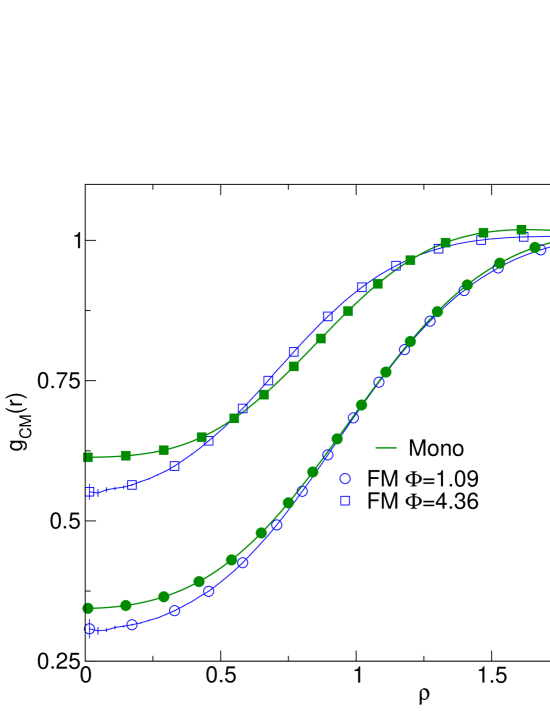 |
Let us finally compare the center-of-mass distribution function . It is reported in figure 9 for and . In the first case, the tetramer result is on top of the polymer results. For small discrepancies at short distance () are present. For instance, for the tetramer we have , at , respectively, to be compared with the polymer results , . These small differences are responsible for the differences in the estimates of since is related to by the compressibility rule444In principle one can use this expression to determine the density derivative of . However, since the relevant length scale for is the average distance between the centers of mass of the polymer chains, finite-size effects will be small only if , where is the size of the box containing the system. On the other hand, if one uses the intermolecular structure factor, the relevant scale is the correlation length , which, in the semidilute regime, is significantly smaller than . Therefore, is smaller than , which implies that determinations using the intermolecular structure factor show smaller finite-size effects than those using .
| (33) |
Note that, even though the thermodynamics is poorly reproduced, also the single-blob model gives an estimate of which is only slightly different from the polymer one. The largest differences are observed for . At overlap we obtain and for and , to be compared with the polymer results and .
4 Comparison with other models
In the previous section, we discussed the finite-density behavior of the tetramer model and we showed that it is quite accurate, for both structural and thermodynamic properties, up to , in agreement with the multiblob argument of Pierleoni et al. [32] presented in the introduction. It represents a significant improvement with respect to the single-blob model, which is unable to reproduce structural properties and reproduces the thermodynamics only deep in the dilute regime (the compressibility factor for the single-blob model differs from the polymer one by less than 5% only for ).
Here we wish to investigate the structural and thermodynamic behavior of two other models discussed in the literature.
4.1 Definition of the models
First, we consider the model introduced by Pierleoni et al. [32] — we name it model M1. A CGBM with blobs is a chain in which neighboring atoms belonging to the same chain interact with an intramolecular potential
| (34) |
atoms that belong to the same chain but are not neighbors, or belong to different chains interact with a potential given by
| (35) |
where and are the same as in (34). In these expressions is the average zero-density radius of gyration of the blobs and sets the length scale. The model depends on several constants, which can be easily determined in the dimer case, i.e., for (see caption of figure 1 in Pierleoni et al.[32]): , , , and . To extend the model to values , Pierleoni et al. [32] made the transferability hypothesis: equations (34) and (35) hold for any , the -dependence being completely taken into account by the radius of gyration of the blob.
As discussed in Sec. 2.2, when comparing the CGBM results to the polymer ones, one should use the radius of gyration of the reference polymer model and not the radius of gyration of the CGBM. The radius (or rather the ratio , since is the basic length scale in this approach) can be determined by using two different routes. As suggested by Pierleoni et al.,[32] one can determine for the CGBM and then use (4). Alternatively one can use (6). If the model were a good CGBM, these two definitions would give the same result, and indeed in the tetramer case they do. Instead, for model M1 we observe quite large differences. For instance, for , we find if we use and , if we use . These differences do not disappear as . An analysis of M1 results with gives for the scaling behavior
| (36) |
which is not compatible with (6).
In this paper we compare the results obtained by using three different “polymer” radii of gyration:
| (37) | |||||
| (38) | |||||
| (39) |
Note that, for large , definitions and are equivalent. On the other hand, as we discussed, definition differs significantly from the others for any , including the limit . Recently, Coluzza et al. [52] suggested that model M1 should not be considered as a CGBM, but rather as a generic polymer model in good-solvent conditions, so that should be used as reference scale. In the following we shall mainly focus on the first and third definition and we shall label the corresponding results as (M1,1) and (M1,3), respectively.
A proper definition of is relevant for two purposes: first, length distributions are universal only if one expresses the lengths in terms of (the relevant scale is ); second, at finite density results should be compared at the same value of the polymer volume fraction defined in (19). Changing the definition of changes the definition of both and , hence it is crucial to specify which one is using. Note that Coluzza et al. [52] introduced a complex procedure to compare CGBM and polymer results. Their procedure is fully equivalent to the one we have discussed above: to analyze finite-density results, one must compare the results at the same value of the adimensional volume fraction .
The thermodynamic behavior of model M1 was studied by Pelissetto.[34] If is used as reference scale as recently suggested by Coluzza et al.,[52] the model fails to reproduce the thermodynamics unless is larger than , but of course, for such values of , there are several other models — the lattice Domb-Joyce model we use is one of them — which better reproduce the universal polymer behavior both for the thermodynamics and the structural properties. For instance, for , which is a relatively large value, model M1 overestimates the second virial coefficient combination by 20%. A more detailed discussion will be presented below.
We shall also consider a second coarse-grained model, [34] we call it model M2. Conceptually, this was not intended to be a CGBM, but rather a polymeric model which reproduces the asymptotic (number of monomers ) behavior already for small values of . The -dependent potentials were tuned so that thermodynamics was reproduced for . For , thermodynamics was reproduced taking potentials of the form (34) and (35) with ( is no longer the blob size, but simply sets the length scale) , , and . It is important to stress that was used as reference length in the optimization procedure employed to determine the optimal parameters. Therefore, for consistency, for this model it makes no sense to use definitions and . Hence, whenever we consider model M2, should always be identified with .
We have performed simulations for model M1 for , 16, 30, 60 and of model M2 for . In the second case, one should in principle compute the appropriate parameters for . We will use here the coefficients computed for , as we expect the changes necessary as goes from 26 to 30 to be tiny.
4.2 Numerical results and discussion
 |
 |
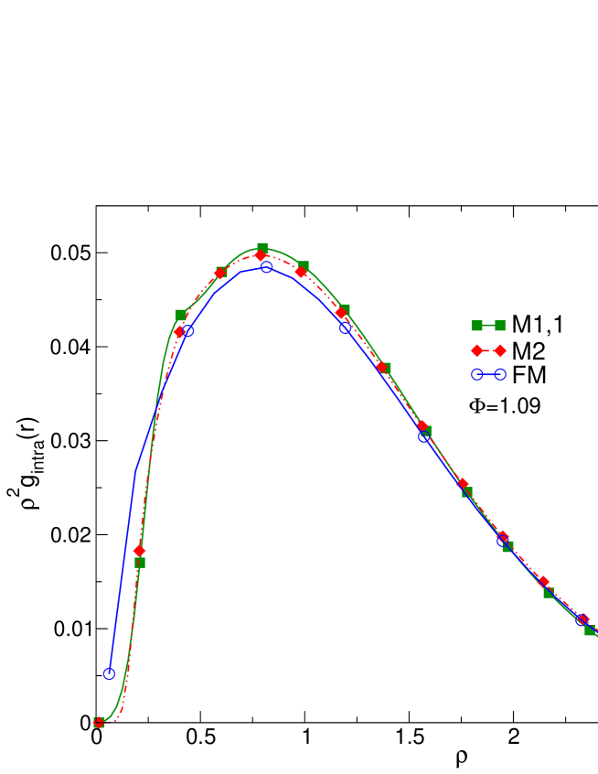
Let us first discuss the structural properties, considering the intramolecular distribution function . If we consider models M1 and M2 as generic polymer models — in this case we should use as length scale — the corresponding results should be compared with the monomer intramolecular distribution function, which is defined in (10), taking . Estimates of , which represents the average distribution of the bond lengths, are shown in figure 10. At , we observe a reasonable agreement for both models: they appear to be able to reproduce the structural properties in the dilute regime. For model M1 shows some, but still reasonably small, differences for . Model M2 appears to be slightly in better agreement, except for small .
 |
 |
 |
 |
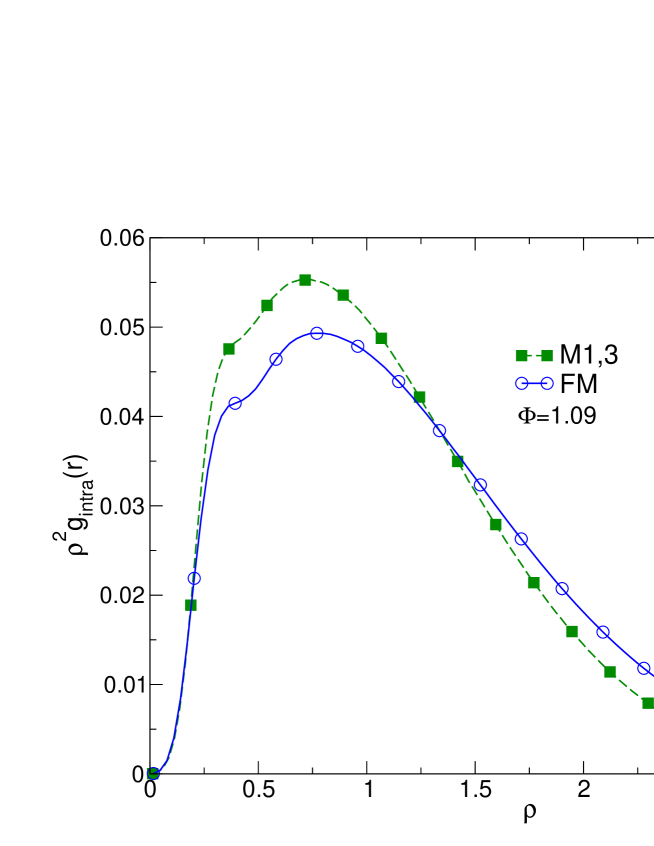
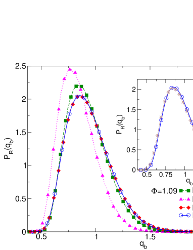
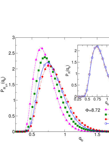
For model M1, we can also consider , see definition (39), for the zero-density radius of gyration. In doing this, we implicitly assume that model M1 is a CGBM, as the tetramer model, and not just a generic good-solvent polymer model. In figure 11 we report the corresponding adimensional intramolecular distribution function, which should be compared in this case with the polymer results for a 30-blob coarse-grained representation (data labelled FM). Discrepancies are significantly larger than in figure 10. Clearly, structural properties are much better reproduced if is used as radius of gyration, in agreement with the conclusions of Coluzza et al. [52] Note that if one uses the M1 distributions agree exactly with the polymer ones for . Indeed, model M1 is, in this limit, a generic polymer model and all models have the same infinite-length behavior as long as the same adimensional quantities are compared. As a consequence, the discrepancies we observe in figure 11 do not decrease as increases. Similar conclusions are reached by considering the distribution of the radius of gyration, see figure 12. Depending on the interpretation of the models as generic polymer models or as CGBMs, one should compare the results with the polymer distributions of or of , where is the radius of gyration of a 30-blob representation of the polymer chain. However, as shown in the inset of figure 12, the two distributions are identical on the scale of the figure, so that this conceptual difference is not relevant in practice. Model M2 appears to be the one which gives the best agreement, but, if is used as a reference scale, also the model-M1 distribution is close to the full-monomer one. If instead is used for model M1, discrepancies are quite large.
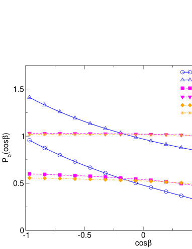
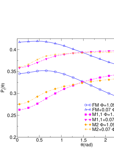
If model M1 is considered as a CGBM, it makes also sense to compare the bending and torsion angle distributions. The results, reported in figure 13, (similar to those observed in model M2) have little relation with what is observed for the polymer case (the full-monomer distributions we report are those appropriate for a 30-blob representation of the polymer). Hence, even if the bond-length distributions are approximately reproduced, correlations between different bonds, for instance angular distributions, are not, and the true polymer shape is quite different from that predicted by model M1.
| 8 | 9.225(7) | 7.729(5) | 5.815(1) | 32.0(5) | 22.4(3) | 12.7(1) |
|---|---|---|---|---|---|---|
| 16 | 8.258(9) | 7.640(8) | 5.548(1) | 26.0(5) | 22.2(4) | 11.7(1) |
| 30 | 7.55(1) | 7.28(1) | 5.354(2) | 21.4(7) | 20.0(7) | 10.8(2) |
| 60 | 6.95(1) | 6.84(1) | 5.183(6) | 17.9(8) | 17.3(7) | 10.0(4) |
 |
 |
 |
Let us now come to the thermodynamics. For both models we have determined the second virial coefficient and the adimensional combination . The parameters of model M2 were determined in such a way to reproduce , the correct result for infinitely long polymers, hence M2 gives the correct thermodynamics in the zero-density limit. The results for model M1 are reported in Table 2 for each choice of . As already discussed by Pelissetto, [34] if is used, differs significantly from the asymptotic result, even for . If is used, discrepancies are smaller for , but substantially the same for (not surprising, since as ). Definition gives apparently better results, but we believe that this apparent agreement is fortuitous. Indeed, as increases, should monotonically decrease, increasing the discrepancy with the polymer case. It is easy to compute the asymptotic value. For large model M1 is a generic good-solvent polymer model, hence standard universality arguments predict that should converge to 5.500, the result obtained for infinitely long polymers. [47]. Using (36) we obtain for
| (40) |
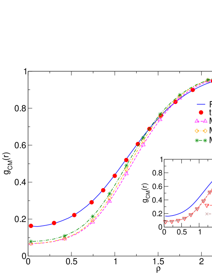
which differs by 25% from the correct result. To further confirm that there is nothing fundamental in the observed agreement, we plot the zero-density center-of-mass distribution function in figure 14. For all values of it differs significantly from the polymer one. In particular, the correlation hole , which does not depend on the choice of , is significantly deeper in model M1 than for good-solvent polymers in the scaling limit.
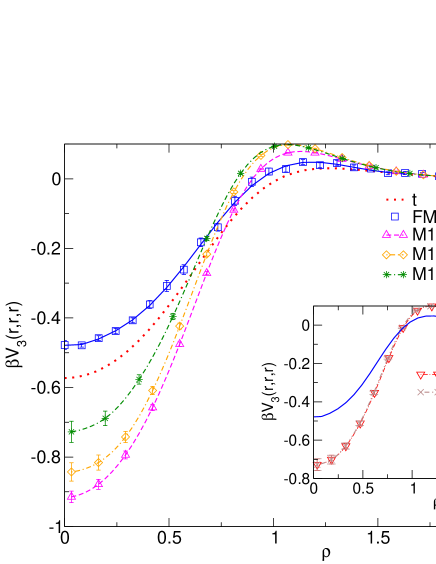
In Table 2 we also report the third-virial combination . If is used, results differ roughly by a factor of two from the polymer ones. Discrepancies decrease if is used, but again this is accidental. The same argument given above for shows that the combination converges to 5.5 for , which is roughly a factor-of-two smaller than the correct result [47] . We also report, see figure 15, the three-body potential of mean force for three chains on an equilateral triangle. We observe significant discrepancies: results are significantly worse than those obtained by using the tetramer CGBM.
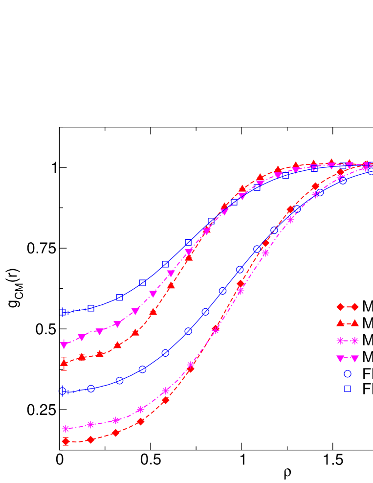 |
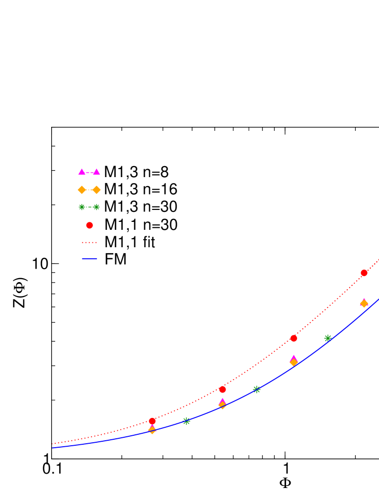
Let us now compare the thermodynamics at finite density. In figure 16 we compare the compressibility factor for polymers (data labelled by FM taken from Pelissetto [48]) with that for model M1. As expected on the basis of the zero-density results, if is used in the definition of , very large discrepancies are observed. Moreover, also the dependence on is incorrect: increases as for , which differs significantly from the correct scaling . Discrepancies are significantly smaller (12% at most, see the right panel of figure 16) if is used. Again the agreement appears to be accidental, since the center-of-mass distribution function differs significantly from the polymer one, see figure 17. Even worse, for , results using appear to be closer to the correct full-monomer results than those obtained by using . Again, note that only if is used the distribution function computed in model M1 will converge to the full-monomer one for . If is used instead, the correlation hole is always (even for ) deeper for model M1 than for true polymers at any given value of the polymer packing fraction . Moreover, shows more curvature, reaching approximately 1 at a slightly smaller value of .
By construction, model M2 reproduces the thermodynamics up to . Indeed, the parameters were fixed by requiring to be equal to the polymer compressibility in the dilute limit and for . Note that it also gives the correct intermolecular pair distribution function, see figure 17, a result which is not a priori obvious.
5 Conclusions
In the last two decades (but the first proposals [53] can be traced back to the ’50s) several coarse-grained models have been proposed for polymers in solution under good- or -solvent conditions. In the simplest approaches polymer chains are mapped onto single atoms interacting by means of soft potentials. These classes of models are however unable to reproduce the structural properties and give the correct thermodynamics only in the dilute limit. To go to higher densities, density-dependent potentials [27, 8] may be used. However, their determination requires in any case finite-density full-monomer simulations, which is what one would like to avoid by using coarse-grained models. Moreover, it is not clear how accurate they are in more complex situations in which polymers only constitute one species in the solution. To overcome these difficulties, the multiblob approach was recently proposed,[32] in which each polymer chain is mapped onto a short linear chain of blobs. This model retains some degrees of freedom and thus it should allow us to obtain the correct thermodynamics even in the semidilute regime. The main difficulty of this approach is the derivation of the intramolecular interactions. In Pierleoni et al.[32] potentials were obtained for any value of on the basis of a transferability hypothesis. However, later[34] it was shown that the resulting model did not have the correct thermodynamic behavior, indicating that much more work was needed to determine the intramolecular interactions.
In this paper we consider again the multiblob approach, determining the intramolecular interactions by matching universal zero-density polymer distributions.555 The polymer distributions are computed by using a lattice model. However, standard renormalization-group arguments allow us to conclude that exactly the same results would be obtained in the limit by using any other — discrete or continuous — model. We map polymer coils onto four-blob chains (tetramers) which interact be means of bonding, bending and torsional angle potentials. They are obtained by requiring the bond-length distributions and the distributions of the bending and torsion angles to be the same in the tetramer and in the full-monomer model at zero density. As for the intermolecular interactions, we only consider pairwise blob-blob interactions, neglecting many-blob potentials. This limits the validity of the model to the regime in which blob-blob overlaps are rare, i.e., to blob volume fractions [ is the blob concentration and ]. For the tetramer this gives .
The tetramer model turns out to be quite accurate up to , in agreement with the argument given above. In this range of densities structural properties as well as the thermodynamics are correctly reproduced. For instance, for the error on is 7%. If we compare the compressibility factor computed in the tetramer model to that determined in the single-blob model we observe a factor-of-three improvement, indicating that the ideas behind the multiblob approach really work. For significant deviations are observed, both for the structure — tetramers are too rigid — and for the thermodynamics — in the tetramer model becomes significanly smaller than for polymers as increases.
We have investigated again the model proposed in [32], model M1, studying in detail structure and thermodynamics. We find that the model cannot be considered as a consistent CGBM, but should rather be thought as a generic polymer model, as recently suggested by Coluzza et al.[52] Since the thermodynamics is poorly reproduced for small values of (we mainly investigate the case ), it is not a surprise that for these numbers of blobs intermolecular correlations are significantly different from those determined in full-monomer simulations with a large number of monomers. On the other hand, internal bond distributions are quite well reproduced. Clearly, for small values of , in spite of the poor thermodynamic behavior, model M1 is able to model correctly some features of the polymer shape, though not all of them — for instance, angle distributions are not reproduced. This is consistent with the results of Coluzza et al.[52] They studied the geometric structure of polymer brushes, comparing results obtained in full-monomer simulations and in model M1. Also in that case, good agreement was observed for some structural properties.
Finally, we consider the model proposed by Pelissetto.[34] In this case, parameters were tuned so that the thermodynamics was exactly reproduced up to . We find that it also reproduces well the intermolecular structure: the polymer center-of-mass distribution function is correctly reproduced in the whole density range . As for the intramolecular structure, we find that the model gives results analogous to those obtained for model M1. Bond-length distributions are approximately reproduced in the density range we have investigated, indicating that also this model correctly reproduces some features of the polymer shape.
In conclusion, we have shown that the newly proposed tetramer model is a significant step forward in the development of a consistent coarse-grained model of polymer chains based on zero-density interactions. To investigate the semidilute regime for large densities, i.e., for , multiblob models with must be developed. In this respect, the most important lesson of the present work is that many-body intramolecular interactions cannot be completely neglected, if one aims at a consistent multiblob model; their absence in model M1 is probably the cause of its failure in reproducing the thermodynamics of polymer solutions. Finally, it would be very important — we leave it for future work — to develop an analogous coarse-graining strategy for chains in conditions. Here single-blob models with pairwise intermolecular interactions fail since thermodynamic stability is only obtained by taking into account three-chain interactions. Since the tetramer model reproduces quite nicely three-chain correlations in the good-solvent regime, it is the good candidate to attack this problem.
Acknowledgements
C.P. is supported by the Italian Institute of Technology (IIT) under the SEED project grant number 259 SIMBEDD – Advanced Computational Methods for Biophysics, Drug Design and Energy Research.
Appendix A The radius of gyration of the blobs: universal predictions
In this appendix we wish to discuss the behavior of the radius of gyration of the blobs. If is the radius of gyration of the -th blob along the chain, the ratio is universal, being an adimensional ratio of large-scale properties of the polymer. It only depends on the position of the blob along the chain, on the number of blobs, and on the density through the polymer volume fraction . Of course, this holds when the number of monomers is large, otherwise scaling corrections should be taken into account. In general we have
| (41) |
where and are universal functions, , see Clisby,[5] is a universal exponent, and a nonuniversal constant that does not depend on , , and , but only on the model. In the polymer model we use at finite density, the Domb-Joyce model with , the constant is approximately zero, so that corrections decay with the next-to-leading exponent .
An approximate expression for the -dependence of the function which works well for is obtained as follows. In the large- limit we have standard Flory scaling, and , with[5] . Now assume that the blob shape and size is not influenced by the neighboring blobs, so that the size of the blob is equal to that of a free polymer with the same number of monomers. We can thus approximate , so that . This formula is of course not exact, since blob-blob interactions cannot be neglected. Still, as we now show, it is reasonably accurate for .
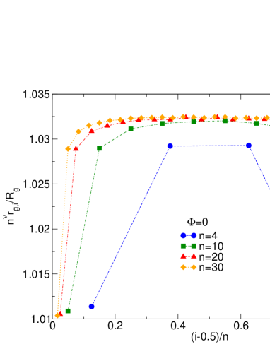 |
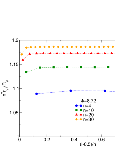 |
In order to compute in the asymptotic limit, we determine for and in the Domb-Joyce model with . Assuming corrections with exponent , we estimate the asymptotic () value as
| (42) |
The combination for is reported in figure 18 as a function of for several values of . Note that this quantity is always larger than 1, indicating that a blob of monomers is more swollen than an isolated chain of the same degree of polymerization. This is due to the neighboring blobs which are entangled with the blob one is considering, causing swelling. Second, this effect is smaller for the boundary blobs since they have only one neighbor. The scaling holds quite well at zero density even for , with a proportionality constant which is only slightly larger than 1. In particular, for the boundary blobs we have , while for the internal blobs . If we average over all blobs and neglect end effects, we obtain relation (6), which we used extensively in the text.
The swelling effect is expected to increase as increases, since the higher the density the higher the blob-blob entanglement is. In figure 18 we also report for . There are here two notable differences with respect to the case . First of all, end effects are small, indicating that much of the swelling is due to neighboring chains, consistently with the idea that for polymers are strongly intertwined. Second, the dependence of the scaling function defined in Eq. (41) is not captured by the simple scaling form for our small values of (of course, scales as for ).
Given the blob radii of gyration, using Eq. (4), we can compute the ratio . For we obtain
| (43) |
Note that the dependence is tiny. At , a good approximation for all is given by
| (44) |
which predicts for for , in good agreement with the result (43).
| 1.09 | 0.982 | 0.990 | 0.994 | 0.996 |
| 4.36 | 0.938 | 0.962 | 0.976 | 0.982 |
| 8.72 | 0.898 | 0.933 | 0.955 | 0.965 |
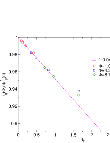 |
It is also interesting to consider the ratio , where is the average blob size in the asymptotic limit (we perform the same extrapolation as done before for the ratios ). Results for several values of and are shown in Table 3 and plotted in figure 19 versus the blob volume fraction . At least for the data appear to depend only on and to converge to 1 linearly as : . Since for at fixed , this result allows us to predict the ratio , the average of the defined above, as . Indeed, we have
| (45) |
The ratio has been computed in several works. [54, 48] For large , scales [48] as so that . Note that scaling (45) sets in for quite large values of if is large. For instance, for it predicts for , since [54] for this value of . Hence, even for , see figure 18, we are still far from the asymptotic limit.
References
References
- [1] P. G. de Gennes, Scaling Concepts in Polymer Physics, Cornell University Press, Ithaca, NY, 1979.
- [2] M. Doi, Introduction to Polymer Physics, Clarendon Press, Oxford, 1992.
- [3] J. des Cloizeaux and G. Jannink, Polymers in Solutions. Their Modelling and Structure, Clarendon Press, Oxford, 1990.
- [4] L. Schäfer, Excluded Volume Effects in Polymer Solutions, Springer, Berlin, 1999.
- [5] N. Clisby, Phys. Rev. Lett., 104, 55702, 2010.
- [6] M. Müller, K. Binder, and L. Schäfer, Macromolecules, 33, 4568, 2000.
- [7] A. Cavallo, M. Müller and K. Binder, Macromolecules, 39, 9539, 2006.
- [8] P. G. Bolhuis, A. A. Louis, J. P. Hansen and E. J. Meijer E J, J. Chem. Phys., 114, 4296, 2001.
- [9] A. A. Louis, P. G. Bolhuis, R. Finken, V. Krakoviack, E. J. Meijer and J. P. Hansen, Physica A, 306, 251, 2002.
- [10] Q. Yan and J. J. de Pablo, J. Chem. Phys., 113, 5954, 2000.
- [11] A. Pelissetto and J.-P. Hansen, J. Chem. Phys., 122, 134904, 2005.
- [12] W. Poon, J. Phys.: Condens. Matter, 14, R859, 2002.
- [13] M. Fuchs and K. Schweizer, J. Phys.: Condens. Matter, 14, R239, 2002.
- [14] R. Tuinier, J. Rieger J and C. G. de Kruif, Adv. Colloid Interface Sci., 103, 1, 2003.
- [15] K. J. Mutch, J. S. van Duijneveldt and J. Eastoe, Soft Matter, 3, 155, 2007.
- [16] P. G. Bolhuis, A. A. Louis and J. P. Hansen, Phys. Rev. Lett., 89, 128302, 2002.
- [17] C. Pierleoni, C. Addison, J.-P. Hansen and V. Krakoviack, Phys. Rev. Lett., 96, 128302, 2006.
- [18] J.-P. Hansen and C. Pearson, Mol. Phys., 104, 3389, 2006.
- [19] J. Sambriski and M. G. Guenza, Phys. Rev. E, 76, 051801, 2007.
- [20] C. Gross and W. Paul, Soft Matter, 6, 3273, 2010.
- [21] F. S. Bates and G. H. Fredrickson, Ann. Rev. Phys. Chem., 41, 525, 1990.
- [22] C. N. Likos, Phys. Rep., 348, 267, 2001.
- [23] M. Dijkstra, R. van Roij, and R. Evans, Phys. Rev. E, 59, 5744, 1999.
- [24] A. Y. Grosberg, P. G. Khalatur and A. R. Khokhlov, Makromol. Chem., Rapid Commun., 3, 709, 1982.
- [25] J. Dautenhahn and C. K. Hall, Macromolecules, 27, 5399, 1994.
- [26] P.G. Bolhuis, A. A. Louis and J. P. Hansen Phys. Rev. E, 64, 021801, 2001.
- [27] A. A. Louis, P. G. Bolhuis, J. P. Hansen and E. J. Meijer, Phys. Rev. Lett., 85, 2522, 2000.
- [28] R. Henderson, Phys. Lett. A, 49, 197, 1974.
- [29] J.-P. Hansen and I. R. McDonald, Theory of Simple Liquids, 3rd ed., Academic Press, Amsterdam, 2006.
- [30] F. H. Stillinger, H. Sakai and S. Torquato, J. Chem. Phys., 117, 288, 2002.
- [31] A. A. Louis, J. Phys.: Condens. Matter, 14, 9187, 2002.
- [32] C. Pierleoni, B. Capone and J. P. Hansen, J. Chem. Phys., 127, 171102, 2007.
- [33] C. Addison, J. P. Hansen, V. Krakoviack, and A. A. Louis, Mol. Phys., 103, 3045, 2005.
- [34] A. Pelissetto, J. Phys.: Condens. Matter, 21, 115108, 2009.
- [35] W. Schommers, Phys. Rev. A, 28, 3599, 1983.
- [36] F. Müller-Plathe, Chem. Phys. Chem., 3, 754, 2002.
- [37] D. Reith, M. Pütz and F. Müller-Plathe, J. Comp. Chem. , 24, 1624, 2003.
- [38] D. Fritz, V. A. Harmandaris, K. Kremer and N. F. A. van der Vegt, Macromolecules, 42, 7579, 2009.
- [39] G. Milano and F. Müller-Plathe, J. Phys. Chem. B, 109, 18609, 2005.
- [40] P. Carbone, H. A. K. Varzaneh, X. Chen and F. Müller-Plathe, J. Chem. Phys., 128, 064904, 2008.
- [41] G. Rossi, L. Monticelli, S. R. Puisto, I. Vattulainen and T. Ala-Nissila, Soft Matter, 7, 698, 2010.
- [42] T. Vettorel, G. Besold and K. Kremer, Soft Matter, 6, 2282, 2010.
- [43] M. Murat and K. Kremer, J. Chem. Phys., 108, 4340, 1998.
- [44] A. J. Clark and M. G. Guenza, J. Chem. Phys., 132, 044902, 2010.
- [45] R. L. C. Akkermans and W. J. Briels, J. Chem. Phys., 114, 1020, 2001.
- [46] R. L. C. Akkermans and W. J. Briels, J. Chem. Phys., 115, 6210, 2001.
- [47] S. Caracciolo, B. M. Mognetti and A. Pelissetto, J. Chem. Phys., 125, 094903, 2006.
- [48] A. Pelissetto, J. Chem. Phys., 129, 044901, 2008.
- [49] G. Ciccotti and J. P. Ryckaert, Comp. Phys. Rep., 4, 346, 1986.
- [50] R. L. C. Akkermans and G. Ciccotti, J. Phys. Chem. B, 108, 6866, 2004.
- [51] A. A. Louis, P. G. Bolhuis and J. P. Hansen, Phys. Rev. E, 62, 7961, 2000.
- [52] I. Coluzza, B. Capone and J.-P. Hansen, Soft Matter, 7, 5255, 2011.
- [53] P. J. Flory and W. R. Krigbaum, J. Chem. Phys., 18, 1086, 1950.
- [54] S. Caracciolo, B. M. Mognetti and A. Pelissetto, J. Chem. Phys., 125, 094904, 2006; (erratum) J. Chem. Phys., 126, 169901, 2007.