Incentives and Redistribution in Homogeneous Bike-Sharing Systems with Stations of Finite Capacity
Abstract.
Bike-sharing systems are becoming important for urban transportation. In such systems, users arrive at a station, take a bike and use it for a while, then return it to another station of their choice. Each station has a finite capacity: it cannot host more bikes than its capacity. We propose a stochastic model of an homogeneous bike-sharing system and study the effect of users random choices on the number of problematic stations, i.e., stations that, at a given time, have no bikes available or no available spots for bikes to be returned to. We quantify the influence of the station capacities, and we compute the fleet size that is optimal in terms of minimizing the proportion of problematic stations. Even in a homogeneous city, the system exhibits a poor performance: the minimal proportion of problematic stations is of the order of (but not lower than) the inverse of the capacity. We show that simple incentives, such as suggesting users to return to the least loaded station among two stations, improve the situation by an exponential factor. We also compute the rate at which bikes have to be redistributed by trucks to insure a given quality of service. This rate is of the order of the inverse of the station capacity. For all cases considered, the fleet size that corresponds to the best performance is half of the total number of spots plus a few more, the value of the few more can be computed in closed-form as a function of the system parameters. It corresponds to the average number of bikes in circulation.
Key words and phrases:
Bike-sharing systems; stochastic model; incentives; redistribution mechanisms; mean-field approximation1. Introduction
Bike-sharing systems (BSS) are becoming important for urban transportation. They are devoted to short trips. A few BSS have been launched since Copenhagen launched its program in 1995. BSS were widely deployed in the 2000s after Paris launched the large-scale program called Velib, in July 2007. Velib consists of 20 000 available bikes and 1500 stations. Currently, there are more than cities equipped with BSS around the world (see [4] for a history of BSS). The popularity of BSS gives rise to a recent research activity.
The concept of BSS is simple: A user arrives at a station, takes a bike, uses it for a while and then returns it to another station. The lack of resources is one of the major issues: a user can arrive at a station that has no bike available, or wants to return her bike at a station with no empty spot. The allocation of resources, bikes and empty places, has to be managed by the operator in order to offer a reliable alternative to other transportation modes.
The strength of such a system is its ability to meet the demand, in bikes and empty spots. This demand is complex. It depends on the time of the day, the day of the week (week or week-end), the season and the weather, but also the location: housing or working areas generate going-and-coming flows; flows are also generated from up-hill to down-hill stations. This creates unbalanced traffic during the day. Moreover, the system is stochastic due to the arrivals at the stations, the origin-destination pairs and the trip lengths. The lack of resources also generates random choices from the users, who must search for another station. These facts are supported by several data analyses, e.g., [1, 9, 21].
When building a bike-sharing system, a first strategic decision is the planning of the number of stations, their locations and their size. Other long-term operation decisions involve static pricing and fixing the number of bikes in the system. Several papers have studied these issues. See [16, 25, 5, 4, 20]. They study the static planning problem based on economical aspects and growth trends. Another important research direction concerns bike repositioning: To solve the problem of unbalanced traffic, bikes can be moved by the operator, either during the night when the traffic is low (static repositioning) or during the day (dynamic repositioning). [23] study the optimal placement of bikes at the beginning of a day. [2] develop an algorithm that minimizes the distance traveled by trucks to achieve a given bike positions, assuming that bikes do not move (e.g., during the night). The dynamic aspects are studied by [3, 24, 22], but their model ignores bike moves between periodical updates of the system. These papers rely mainly on optimization techniques.
Redistribution can also be done by users. In most BSS, users have access to the real-time state of the stations, e.g., by using a smartphone. They can choose to take or to return their bikes to a station near their destinations. Moreover they can be encouraged to do so by the system. For example, Paris, via the Velib+ system, offers a static reward by giving free time slots in order to bring more bikes to up-hill stations. It is estimated that the number of people that obtain rewards via Velib+ during the day is equivalent to the number of bikes redistributed by trucks. To compensate for real-time congestion problems, an alternative is to use real-time pricing mechanisms. This type of congestion control mechanism is widely applied in the transportation or car-rental industry, e.g., [15, 27]. Nevertheless, its application to BSS is unclear, as the price paid per trip for using BSS is usually low.
A few papers tackle the stochasticity of BSS, or more generally of vehicle rental systems (see [14, 13] and literature therein). Their first idea was to obtain a simplified asymptotic behavior when the system gets large. This approximation is valid as BSS are large systems and can give qualitative and quantitative properties for the model. In models with product-form steady-state distribution (see [12, 13]), the asymptotic expansion of the partition function can be obtained via complex analysis (saddle point method), see [18], or probabilistic tools, see [6]. One of the main limitations of these papers is that they ignore that stations have finite capacities and therefore neglect the saturation effect.
Contributions – We present a model of a bike-sharing system and analyze its steady-state performance. The system is composed of a large number of stations and a fleet of bikes. Each station can host a finite number of bikes , called its capacity. We measure the performance in terms of proportion of so-called problematic stations, i.e., stations with no available bikes or no empty spots.
We study an homogeneous scenario, in which all stations have the same parameters. Our aim is to obtain a simple tractable model. Intuitively, this system in which the flow of bikes between two stations is, on average, identical in both directions, has roughly speaking the best behavior. For more details, see our work on inhomogeneous BSS, [7]. We investigate the effects of random choices of users and characterize the influence of the station capacity on the performance. We compare incentives and redistribution mechanisms, and we obtain closed-form characteristics of their performance. This model can be straightforwardly extended to model non-homogeneous cities in order to take into account the difference of attractiveness among the stations. The paper by [7] provides analytical results in the case where the stations can be grouped into clusters of stations that have the same characteristics. These results will be briefly presented and discussed in this paper. The redistribution and incentive mechanisms in an heterogeneous setting are not studied by [7] but will be included in their upcoming paper, [8].
This homogeneous model also forgets geometry, present in real-world systems where the bikes are returned to neighboring stations in case of lack of available spots. But the homogeneous model study is nevertheless useful: simulations show that the behavior of both systems are very similar. Thus the qualitative and quantitative results obtained for the homogeneous model apply to a system with a local search of an empty spot.
Our first contribution is to study the simplest model without any incentives or redistribution mechanisms. We use a mean-field approximation that enables us to obtain the asymptotic behavior of our model as the system size becomes large. This asymptotic dynamics leads to simple expressions that give qualitative and quantitative results. This method works even if a closed-form (product-form) expression is not available for the original model. We show that the proportion of problematic stations depends on the fleet size and it decreases slowly with the capacity . For a given capacity, it presents a minimum that is attained at a fleet size called optimally reliable fleet size, which is equal to bikes per station, where is the arrival rate of users at a station and is the average trip time. This answers the fleet sizing problem. The term represents the average number of bikes in circulation. It quantifies the intuitive idea that the greater the demand is, the more bikes must be put in the system. For this fleet size, the proportion of problematic stations is .
To improve the situation, we investigate two different directions: incentives and redistribution. We first assume that users have access to real-time information on the system and follow the rules the system gives about where to take or return the bike. The improvement that is obtained in this case is quantified. We show that returning bikes to a non-saturated station does not change significantly the behavior of the stations and the performance with our metric. The situation improves dramatically when users return their bikes to the least loaded station among two, even if only a fraction of the users do this. Indeed we prove that, if all users do this, the proportion of problematic stations can be as low as . These results are confirmed by simulations in which users choose among two neighboring stations. Again, the optimally reliable fleet size is a little more than .
In Section 5, we then study what we call the redistribution rate . We define the redistribution rate as the ratio of the number of bikes that have to be moved manually by trucks over the number of bikes that are taken by users. It is proved that the redistribution rate that optimizes performance depends on the fleet size and the station capacity. More precisely, the redistribution rate threshold needed to suppress problematic stations is minimal when the fleet size is bikes per station and is equal to .
Finally, in Section 6, we discuss the limitations of the model. We describe briefly the differences that will occur when considering a time- or space-inhomogeneous model. We mainly refer to the paper by [7], whose main result is an extension of the expression of the minimal proportion of problematic stations within a cluster at some optimally reliable fleet size, which generalizes . We also show simulation results of more realistic models that consider various trip-time distributions and take the geometry into account. In all cases, these models behave similarly to the original model. We also simulate a two-choice model where the choice is made at the beginning of the trip, when taking the bike. We introduce then a different performance indicator, the average number of stations visited before returning a bike. We show that, except when the system’s geometry is a line, this indicator can be deduced from the proportion of saturated stations. Moreover we show that our model can be extended, while remaining analytically tractable. We detail the case of mean search times that are shorter than the mean travel time, and the case of losses of users arriving at an empty station are replaced by a search of an available bike in another station. These extensions have also been investigated by simulation on models with geometry. Their behaviors are still very similar.
Organization of the Paper – Section 2 presents the model description and the mean-field techniques. Section 3 deals with the basic model results. Section 4 studies incentive mechanisms where a fraction of users choose the least loaded of two stations to return their bike. Section 5 shows that there exists a threshold for the rate of redistribution by trucks which optimizes performance. Section 6 deals with discussions, extensions and simulation validations. Section 7 concludes.
2. System Model and Mean-Field Analysis
In this section, we present the basic model. Mean-field techniques are used to investigate the performance of homogeneous BSS. These techniques reduce the study of the stochastic model to the study of the equilibrium point of a set of differential equations. We detail the steps to obtain this result. The other scenarios studied in this paper fit the same framework.
2.1. Main Notation List
| Number of stations. | |
| Average number of bikes per station (the total number of bikes is ). | |
| Number of slots in a station, also called capacity of the station. | |
| Arrival rate of users at a station. | |
| Average trip time. | |
| Proportion of the stations where bikes are available at time . | |
| Limit of as tends to infinity (described by an ODE). |
| Equilibrium point of the corresponding ODE. | |
| Proportion of the stations where or more bikes are available at . | |
| Limit of as tends to infinity (described by an ODE). | |
| Equilibrium point of the corresponding ODE. |
2.2. Homogeneous Bike-Sharing Model
We consider a Markovian model of a bike-sharing system with stations and a fleet of bikes ( bikes per station in average). A bike can be either hosted at a station or in transit between two stations. In this paper, we focus on the homogeneous bike-sharing model. It allows us to obtain a closed-form expression for the optimal performance and also, in the next sections, to investigate incentives and redistribution by trucks in this framework, and to quantify their effects. This study is extended to an inhomogeneous model by [7].
Each station can host bikes. At each station, new users arrive at rate . If there is no bike at this station, the unhappy user leaves the system. If the station is not empty, the user takes a bike at this station and joins the pool of riding users. The trip time between the two stations is exponentially distributed with mean .
After this time, the riding user wants to return her bike. She chooses a destination at random among all stations. If her destination has fewer than bikes, the user returns her bike to this station and leaves the system. If the station has bikes, no more bikes can be returned at this station and this station is called saturated. In this case, the user rides to another station. This station is again chosen at random and the trip time is exponentially distributed with mean . This process is repeated until she finds a non-saturated station.
As seen in the rest of the paper, our model can be thoroughly analyzed and leads to closed-form results. This model, however, does not incorporate any geographical information. In a real-world system, users who cannot find a bike or cannot return their bike will try a neighboring station and not just one at random. These modifications unfortunately lead to intractable models. Nevertheless, we show by using simulations in Section 6 that taking into account locality has little effect on the overall performance.
2.3. Mean-Field Limit and Steady-State Behavior
In this section, we prove that the analysis of the system is essentially the analysis of an ordinary differential equation (ODE) as goes to infinity and that the equilibrium point can be addressed.
Let us denote by the proportion of stations where bikes are available at time . As the system is homogeneous, the process is a Markov process. Suppose the process is at . There are two types of transitions:
-
•
Bikes taken. The arrival rate of users in a station that has bikes is . When , it causes the th coordinate, , to decrease by and to increase by .
-
•
Bikes returned. The number of bikes in transit is equal to the total fleet size minus the number of bikes hosted at the stations, which is equal to . As trip times are exponentially distributed with mean and stations are chosen at random, a user arrives with a bike at a station with bikes at rate . When , this causes to decrease by and to increase by .
The transitions can be summarized by
where the -th unit vector of is denoted by and is equal to 1 when and otherwise.
This process belongs to the family of density-dependent population processes, defined by [17]. This means that there exist a set of vector and a set of functions such that the transitions are of the form and occur at rate . This implies that, from , the average change in a small interval is . As is Lipschitz-continuous, it is shown in [17] that as goes to infinity, for each , the process converges in distribution to a deterministic function , which is the unique solution of the following differential system of equations:
| (1) |
where is the -th unit vector of .
The first term corresponds to the rate of arrival of new users at a station, and the second term corresponds to the rate at which users return bikes, which is times the proportion of bikes in transit at time .
The above differential equation rewrites where the is the product of the row vector , by the jump matrix . This equation contains the mean-field property of the model: this means that, when tends to infinity, the empirical distribution of the stations evolves in time as the distribution of some non-homogeneous Markov process on , whose jumps are given by , updated by the current distribution . These jumps rates are those of an queue, where the arrival rate is time dependent and the service rate is . This queue represents the instantaneous evolution of any station, because all the stations have the same evolution due to the homogeneity.
Throughout the paper, we investigate the steady-state behavior of the system. For all variants of the model studied in this paper, the dynamical system has a unique equilibrium point. Note that this fact alone does not imply that the sequence of invariant measures of concentrates on this fixed point: it is necessary to show that the dynamical system does not have long-term oscillations and, in general, the proof of this is difficult. There are different techniques for obtaining this result. In Section 3, we show the absence of oscillations by using a generic Lyapunov function. Although numerical evidences show that this is also the case for the other models, the proof is out of the scope of the paper and the question is not addressed for models with incentives or redistribution.
2.4. Performance Metric and Proportion of Problematic Stations
In this paper, we mainly focus on a quality of service indicator, called the proportion of problematic stations. This proportion is the proportion of stations where either no bikes are available or that are saturated. When the number of stations goes to infinity, this proportion converges to , where is the unique fixed point of the differential equation.
This metric generalizes the loss probability, used for example in the context of vehicle rental networks by [12], where the station capacities are infinite. Moreover, a user will be satisfied if she can take a bike at her chosen place of departure and return it at her chosen destination. In an homogeneous system like ours and if origin and destination are chosen uniformly at random, this occurs with probability . Hence, our metric is close to the limiting proportion of unsatisfied users, who cannot enter the system or return their bike in the station of their choice. It measures the quality of service in [27] and [20]. The average sojourn time in the system can also be deduced from and . When a user wants to return a bike at a
saturated station, she has to find a non-saturated station. When this search is done at random, the average number of stations that are visited before finding a spot is (see details in Section 6.3.1). In Section 6.3, we show that, for a realistic model of geometry (2D grid), the average number of visited stations is close to .
This justifies the choice of this simple metric, though others can be deduced from and . Indeed, the sum hides the relative value of each term, which can be useful to know. Nevertheless, this has the advantage of providing a single indicator of the performance. Our goal in this paper is to obtain bounds on this performance criteria. The proportion of problematic stations is not a cost function. In this paper, we do not question the cost or the practical methods for implementing our mechanisms and leave this question for future work. Hence, throughout the paper, the term optimal performance will be understood in term of minimizing this quality of service. It occurs for a value of the fleet size called optimally reliable fleet size.
3. Basic Model and Optimal Fleet Size
This section is devoted to the basic model. As seen in Section 2.3, the behavior of the system can be approximated by the ODE (1) when the system becomes large. This allows for a complete study of the performance metric as a function of . We derive the optimal reliable fleet ratio and discuss the influence of the parameters and .
3.1. Basic Model: Steady-State Analysis
An equilibrium point of the ODE (1) is the stationary measure of an queue with arrival rate and service rate . For , let be the invariant probability measure111For , is the uniform distribution on . For , is geometric: where is the normalizing constant. of a queue with arrival-to-service rate ratio and define . The equilibrium points of (1) are thus the solutions of the fixed point equation .
We now prove the existence and uniqueness of the equilibrium point. For each , there exists a unique stationary measure . Hence, this equation is equivalent to where is the solution of
| (2) |
This equation can be easily explained. The proportion of bikes per station is the sum of two terms: The mean number of users still riding, , and the mean number of bikes per station, . The expression of first term can be computed using the arrival rate and the probability of finding an available bike at a station, . Returning a bike at the -th attempt takes an average time and occurs with probability . Thus, the first term is equal to , which reduces, after some computation, to .
The right part of Equation (2) strictly increases in . Therefore, for each , there is a unique solution of equation (2) and thus a unique equilibrium point is denoted by in the following.
In [7], we exhibit a Lyapunov function for this dynamics in a more general setting. It shows that all trajectories of the ODE converge to the unique fixed point. As a consequence, the steady-state empirical distribution of the system concentrates on this unique fixed point. This means that the limiting stationary distribution of the number of bikes at a station is this fixed point, i.e., a geometric distribution on where the parameter is the solution of Equation (2).
3.2. Proportion of Problematic Stations
The next theorem shows the effect of the number of bikes per station on the performance of the system. Let be the equilibrium point of the equation. The fixed point of Equation (1) can be rewritten as a polynomial equation in of order . Hence, even if solving this equation is possible for very small values of , finding a closed-from expression for is unfeasible. Nevertheless, Equation (2) provides an efficient way to achieve a performance study of the system by considering the parametric curve
| (3) |
where, and in the following, is equal to . The use of this parametric curve allows us to study efficiently the performance of the system as a function of the number of bikes per station . These results are summarized in the next theorem and in Figure 1.
Theorem 1.
For the homogeneous model,
-
(i)
the limiting proportion of problematic stations, , is minimal when and the minimum is equal to . It goes to one when goes to zero or infinity.
-
(ii)
As grows, the performance around becomes flatter and insensitive to and .
Proof.
Let and . Functions and are well defined on . The proportion of problematic stations as a function of is given by . First we prove that has a minimum at which is . For that, differentiating function with respect to gives
Differentiating the numerator and studying the variation, it holds that the numerator strictly increases on and . Thus strictly decreases on , strictly increases on and has a minimum at which is . This shows the optimal number of bikes per station corresponds to , and thus is the optimal reliable proportion of bikes per station. This leads to a proportion of problematic stations of and concludes the proof of (i).
To prove (ii), note that the second derivative of at is . An asymptotic expansion of at is given by
and therefore Moreover, differentiating gives that which leads to
This means that is never sharp for the range of values considered in this paper, i.e., . Moreover, goes quickly to as grows. ∎∎
This theorem indicates that, even for a homogeneous system for which the number of bikes per station is chosen knowing all parameters of the users, the proportion of problematic stations decreases only at rate . This is problematic for practical situations where, for space constraints and construction costs, station capacities are often fewer than 20 or 30 bikes. A system with bikes per station would lead to a proportion of problematic stations of . Although it might be acceptable if this bike-sharing system is used only once in a while, a probability of for a station to be problematic is too large for a reliable daily mode of transportation.
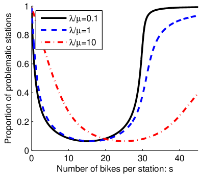
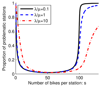
The results of Theorem 1 are illustrated by Figure 1, which plots the performance as the parametric curve given by Equation (3) for two values of the station capacity and three values of .
When is fixed to and , the performance is almost equally good with to bikes per station (i.e., ). However, as soon as the number of bikes per station is lower or higher, the performance decreases significantly. The problematic case is mainly due to empty stations at low versus saturated ones at large . When the size of the stations is , the performance is less sensitive to the number of bikes per station. As pointed out by Theorem 1, in this case, the proportion of problematic stations is : Multiplying the station capacity by divides by the minimum proportion of problematic stations. Having some stations designed to host up to bikes is realistic for stations near a subway for example, but having all stations in a city with slots is very costly in terms of space and installation.
When , the situation is similar to the case , with curves shifted to the right. The minimum number of problematic stations is the same, only the optimal reliable fleet size is changed. This can be deduced from (3) as the term affects only and not the proportion of problematic stations .
These results suggest that without incentives for users to return their bikes to a non-saturated station or without any load-balancing mechanisms, the implementation of a bike-sharing system will always observe a poor performance, even if the system is homogeneous and there are no preferred areas. In a real system where some regions are more crowded than others (e.g., because of the trips from residential areas to work areas), the situation can only be worse. See [7] for a study. In the following, we will examine simple mechanisms that improve dramatically the situation.
3.3. If People Return the Bikes to a Non-saturated Station
Before studying incentive or regulation mechanisms, in this section we study a variant of the model where users know which stations are empty or saturated. They always arrive to non-empty stations and return their bikes only to non-saturated stations.
The dynamics of the system are slightly modified as follows. As before, there is a Poisson arrival process in the system at rate , but each arriving user picks at random a station among the non-empty stations. If there are no non-empty stations, she leaves the system. If the user manages to find a bike, then after a time exponentially distributed with parameter , she arrives at a non-saturated station picked at random (i.e., with fewer than bikes), returns her bike at this station and leaves the system. Note that there is always a non-saturated station (this is the case if ).
The transitions of are now given by
The differential equation is replaced by where
The function is discontinuous when goes to or when goes to . Nevertheless, it can be shown with elementary arguments that if then the differential equation has a unique solution. In the following, we assume that . As for the previous model, equation can be rewritten as . This time, is the infinitesimal generator of an queue with arrival rate and service rate .
By the same method as in the previous section, it can be proved that the dynamical system has a unique fixed point , which is solution of the equation . Moreover, following the same lines as Tibi [26, Proposition 4.3], the steady-state, denoted by , converges as gets large, to this fixed point. The limiting steady-state of the number of bikes at a station is, again, geometrically distributed, with parameter given by the previous equation. The fact that the term is replaced here by can be simply explained. Each user is accepted in the system and returns the bike after one trip with mean time . There are, on average, users riding per station.
When studying the fixed point of the system, we find that the main difference with the original model studied in Section 3.2 is the expression of . Therefore, the performance of the system is easily plotted by a parametric curve similar to (3).
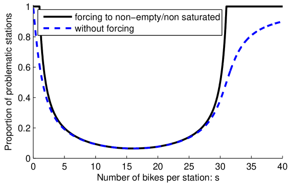 |
The proportion of problematic stations has a similar shape for this model and the one of the previous section. As before, the minimal proportion is and is attained for . When is not equal to , this proportion will be higher than in the classic model. This is illustrated in Figure 2 where the proportion of problematic stations for that model is compared with the model studied in Section 3.1. For small , the less satisfactory behavior of the regulated system is due to the fact that every user can enter the system. This resembles the influence of a larger in Figure 1. For large , this poor behavior of the system is related to the improvement on the customer trip time. It has the same effect as the influence of in the basic system.
This shows that although forcing people to go to a non-saturated or non-empty station reduces the unhappy users because anyone can take or leave a bike at anytime, it makes the system more congested and degredate the situation for users who are not aware of such mechanisms.
4. Incentives and the Power of Two Choices
In this section, we consider that, when a user wants to return her bike somewhere, she indicates two stations and the bike-sharing system indicates to her which one of the two has the least number of bikes available. We show that, when the two stations are picked at random, the proportion of problematic stations diminishes as (instead of in the original model). The performance is thus improved dramatically, and even if only a small percentage of users obey this rule. This result is similar to the well-known power of two choices that has been proved to be a very efficient load balancing strategy, see [19].
4.1. The Two-Choice Model and Its Steady-State Analysis
We consider an homogeneous model with stations and bikes per station. As before, users arrive at rate in each station and take a bike if the station is not empty. Otherwise, they leave the system. When a user chooses her destination, instead of choosing one station, she picks two stations at random, travels and returns the bike to the one that has the lowest number of bikes available.
Let be the proportion of stations with or more bikes at time () i.e., . The state of the system can be described by the vector that is such that .
There are two types of transitions for the Markov process. Suppose is at . The first one is a transition from to , when a user that takes a bike from a station with bikes. This happens at rate . The second type is a transition from to , when a user returns a bike. The number of bikes locked at stations is . Hence, there are bikes in transit. As a user chooses the least loaded among two stations, a user returns a bike at a station with bikes at rate . As in Section 2, as grows large, the behavior of the system can be approximated by the dynamics of the following ODE:
| (4) |
for and and for .
The following theorem shows that these incentives dramatically improve the performance compared to the original model where users go to a station at random (Theorem 1). For a given capacity , the optimal proportion of problematic stations goes from in the original model to .
Theorem 2.
Assume that all users obey to the two-choice rule. Then, the corresponding dynamical system, given by (4) has a unique fixed point. The proportion of problematic stations is lower than for all .
Proof.
First show that the ODE (4) has a unique fixed point. Let . The key point is to reduce the equation giving the fixed point to a first order recurrence equation. Indeed, a direct recurrence gives that a fixed point must satisfy and for all :
| (5) |
with .
For all and , define by and . By induction on , there is a increasing sequence such that is strictly increasing on and . Indeed,
-
•
This is true for because .
-
•
Then, if it is true for some , then is increasing on because is increasing and positive on . Moreover, and .
This shows that there exists a unique such that on .
A fixed point of Equation (4) is a vector such that and . By the property stated above, for a fixed , there is a unique fixed point, which is . Moreover, is increasing in , which implies that there is a unique fixed point when is fixed.
Let and assume that . If , a direct recurrence shows that for , which contradicts the fact that . Therefore, . Hence, for all ,
which implies that . As , using Equation (5),
| (6) |
Let and . Using Equation (6),
| (7) |
If , then , which is less than for all . This contradicts Equation (7) and shows that .
The proportion of empty stations is . The proportion of saturated stations is , which is such that . Thus, . This shows that, for all , the proportion of problematic stations is less than
This quantity is less than for all and is asymptotically equivalent to .
The fleet size , equal to , is an increasing function of . Moreover, Hence, when ,
This shows that if , .
When , a direct induction on shows that . Let be such that . For such a , . Hence
This implies that, for all , .∎∎
Assume now that only a fraction of the users follow this rule and that the others go to a station at random. This could happen if the users are rewarded, when they obey the two-choice rule, like in the Velib+ system. To model this behavior, we assume that each user obeys to the two-choice rule with probability and otherwise chooses only one station and returns the bike to it. The dynamics are similar to Equation (4) and an equilibrium point satisfies the following equations: and
| (8) |
In this case, the fixed point Equation (5) becomes . The proof of the uniqueness of the solution of Equation (5) can be easily adapted to show that Equation (8) also has a unique fixed point.
4.2. Impact on the Performance
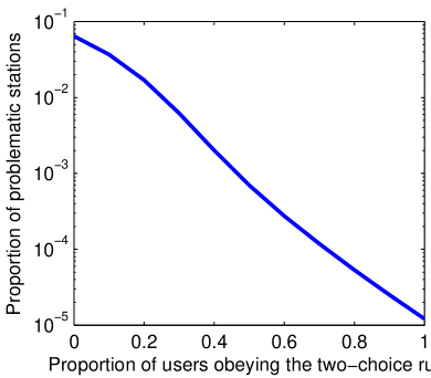
Due to the uniqueness of the solution , the proof of Theorem 2, especially Equation (5), provides an efficient way to compute as a function of . This shows that, if is fixed, the number of bikes in the system is . The performance indicator can be plotted by using a parametric curve of parameter . These results are reported in Figure 3 and indicate that the performance of the system is radically improved compared to the original case (Figure 1), even if of users obey the two-choice rule.
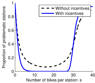
In Figure 3(a) we report the proportion of problematic stations as a function of the proportion of bikes per station when everyone follows the two-choice rule. We observe that the optimal performance of the system is much better than in the original system (here and ). Although in the original system, the proportion of problematic stations is at best around , here the proportion of problematic stations can be as low as (this is lower than the bound of Theorem 2, which is ). Moreover, this curve is rather insensitive to variations in the number of bikes: The proportion of problematic stations is less than if is between and bikes. An interesting phenomenon occurs when the average number of bikes per station exceeds the capacity of the station. In this case, there is a larger proportion of problematic stations for the two-choice model than for the original situation. This is explained by the fact that when a user obeys the two-choice rule, it is easier for her to return a bike. Hence, when more users obey the two-choice rule, there are fewer bikes in transit and the stations are more occupied. This negative effect only occurs when , which confirms Theorem 2: Performance is low for less than a value close to .
On Figure 3(b), the average number of bikes per station is fixed, , and the proportion of users who obey the two-choice rule varies from to . This shows that the proportion of problematic stations diminishes rapidly as soon as the number of users obeying the rule grows. Moreover, the decrease is approximately exponential: if more users obey the rule, the proportion of problematic stations is roughly divided by .
5. Optimal Redistribution Rate
Balancing the number of bikes in various areas in a city is one of the major issues of bike-sharing systems. A widely adopted solution is the use of trucks to move bikes from saturated stations to empty ones. This redistribution mechanism can equalize the one-directional flows of travelers, for example from residential areas to work areas, but also the imbalances due to the choices of users. In this section the minimal redistribution rate needed to suppress any problematic station is investigated, and we conclude by showing that it decreases as the inverse of the station capacity. Our analysis assumes that bikes are moved one by one. This assumption will be relaxed in simulations in Section 6.5, thus showing that a larger truck size does not affect qualitatively the performance.
5.1. The Redistribution Model and Its Steady-State Analysis
We consider a homogeneous model of bike-sharing systems with stations equipped with a truck that visits the stations to adjust their load. The user behavior is the same as in Section 2. The arrival rate at any station is and a bike trip takes a time exponentially distributed of mean . A truck knows the station occupancies at any time. It goes to the most loaded station, takes a bike and returns it to the least loaded station. The trip time of the truck is neglected (the bikes are assumed to move instantaneously from highly loaded to lightly loaded stations). This description amounts to one truck that moves bikes at rate . The resulting Markov model is the same if there is trucks moving bikes at rate . In the rest of the section, we study the effect on the performance of the ratio . This ratio is the average number of bikes per second that are moved manually by the operator divided by the number of bikes per second taken by regular users.
As in Section 4, let be the proportion of stations that have bikes or more available at time . In particular, and . There are three kinds of transitions in the system: arrivals and departures of users and redistribution. The fluid model transitions corresponding to the user arrivals and departures are the same as in Equation (1) with a number of bikes in transit of . Moreover, the redistribution part only affects the most loaded and least loaded stations, i.e., stations that have bikes available, where is such that no stations have less less than bikes available () or no stations have more than bikes available (). This shows that the expected variation of during a small time interval is equal to , where for all ,
The function is not continuous in . Hence, the ODE is not well defined and can have zero solutions. To overcome this discontinuity problem, it has been shown by [10, 11], that this ODE can be replaced by a differential inclusion , where is the convex closure of the set of values for in a neighborhood of . This differential inclusion is a good approximation of the stochastic system as grows. In particular, as with classic ODE, if all the solutions of the differential inclusion converge to a fixed point, then their stationary measures concentrate on this point as goes to infinity, see [11].
In our present case, the differential inclusion is
| (9) | ||||
| (14) |
To ease the presentation, the details of its construction are omitted. The construction is similar to Section 4.3 of [11]. This leads to the following result.
Theorem 3.
Assume that a truck moves bikes from the most loaded station to the least loaded one at rate . If and then the fixed point of the dynamical system (9) satisfies:
-
•
If , then there is no problematic station.
-
•
If , the proportion of problematic stations decreases with .
The quantity is called the optimal redistribution rate. Setting is not necessarily optimal in terms of cost but it corresponds to a key of the performance: When , the proportion of problematic station decreases almost linearly and is zero when .
Proof.
Let us assume that . The other case is symmetric and can be treated similarly. The proportion of problematic stations is non-increasing in the redistribution rate . We define the vector by
Let us show that when , is a fixed point of the differential inclusion (9), i.e., there exists such that Equation (9) is equal to zero. Let be a vector such that , , and otherwise. The vector belongs to , defined in Equation (9).
Moreover, by a direct computation,
In particular, . Plugging it in Equation (9),
-
•
for , .
-
•
for , .
-
•
for ,
-
•
for ,
This proves that is a fixed point of the differential inclusion (9). Using monotonicity arguments as in Theorem 2, we can show that this fixed point is unique. However, the proof is quite technical, hence omitted. As the proportion of problematic stations is zero for , this concludes the proof of the theorem.
We now consider the case (which corresponds to and ). Define and a sequence :
-
•
If , then define for and .
-
•
Otherwise, let and
It is straightforward to verify that for all , is a fixed point of the differential equation (9). Moreover, the quantity is an increasing function of . This shows that the differential equation has a unique fixed point (for ). ∎∎
5.2. Impact on the Performance
Theorem 3 shows that the optimal redistribution rate decreases with the station capacity. The optimal redistribution rate is minimal for . In this case, moving bikes from saturated to empty stations at rate suffices to avoid the existence of problematic stations. When is an integer, the optimal redistribution rate simplifies in .
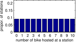
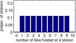
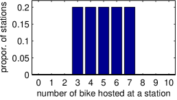
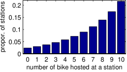
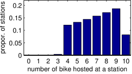
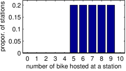
These results are illustrated in Figure 4. The station capacity is set to and (the trip time is negligible). The proportion of stations that have bikes available is plotted as a function of . Two fleet sizes and are compared, according to various values of : , (the optimal redistribution rate for ) and (the optimal redistribution rate for ).
In both cases, the occupancy distribution concentrates around as increases. When , the occupancy distribution is uniform for . As expected, there is no problematic station when . When , the occupancy distribution is geometric for (see Section 3.1). For , there is no empty station and the occupancy distribution is truncated geometric. When , the occupancy distribution is uniform on and there is no problematic station.
6. Validation of the Model: Extensions and Simulations
6.1. Time- and Space-Inhomogeneous Systems
In this paper, we focus on homogeneous bike-sharing systems. This means that the travel demand is constant with time and that this time is the same for any pair of origin and destination. The model presented in Section 3.1 captures the main features of these systems, i.e., loss of the arriving users, search when returning a bike. As we consider a homogeneous model, its performance is naturally described in terms of the proportion of problematic stations in steady-state.
A natural extension of these results is to consider space-inhomogeneity and time-inhomogeneity. Space-inhomogeneity often occurs in cities where some stations are geographically higher or lower than others, thus creating a flow from one region of the city to another. Our basic model can be directly extended to this case, for example, by considering clusters of stations that have a similar level of popularity. The steady-state behavior of such a model is exposed by [7]. This enables us to compute the fleet size that is optimal in terms of minimizing the proportion of problematic stations in a given cluster. Because of working hours or week-ends, bike-sharing systems are often time-inhomogeneous. Modeling these phenomena can be done by considering tides of people that go from housing to working areas in the morning and come back in the evening, as in [28]. In this case, the proportion of
problematic stations does not reflect the performance of the system and the definition of a performance metric is not clear and might depend on the situation. Characterizing and understanding such systems is an issue beyond the scope of this paper, and we plan to tackle it in future work.
6.2. Distribution of Trip Times
6.2.1. One-Choice Model: Insensibility to the Distribution of Trip Times
In order to obtain a tractable model, we choose the inter-arrival times of users and trip times to be exponentially distributed. This leads to a Markovian model that has a compact representation. We investigate the influence of more realistic distributions by using simulation. Our preliminary simulation results indicate that if the average trip time has an influence on the performance, the actual distribution has little effect. The behavior of a system with general trip-time distribution is very similar to a system where trip times have an exponential distribution with the same mean.
To verify this assumption, we compare four possible trip-time distributions:
-
(1)
Original model – The trip times are exponentially distributed of mean .
-
(2)
Deterministic – The trip times are all equal to .
-
(3)
Log-normal – The trip times follow a log-normal distribution of mean and standard deviation .
-
(4)
Uniform – The trip times are uniformly distributed on .
In all cases, the average trip time is . We simulate the four cases on a system composed of stations. Apart from the trip distribution, the model is exactly the same as in Section 2.2 (users arrive according to a Poisson process and there is no geometry). The results are reported in Figure 5.
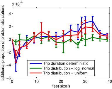
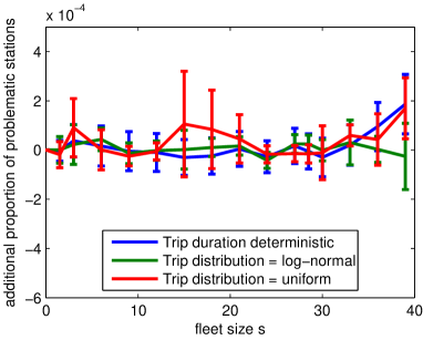
For each distribution, we plot the proportion of problematic stations for this distribution minus the proportion of problematic stations for the original model. The results are shown as a function of the fleet size for two situations: (Figure 5(b)) and (Figure 5(b)). The results reported in Figure 5 are the average over 100 simulations. The errorbars are the 95% confidence interval. We observe that, for a fixed value of , the average difference is always small and is almost smaller than the confidence interval. However, we recall that the average trip duration does have an influence (see Figure 1 and Figure 10).
We conclude that the trip distribution has a negligible effect on the performance. The performance of the system depends only on the average trip time . Note that we also simulate a case where the trip time is exponentially distributed but when the time between two arrivals of customers follows one of the four distributions. The results, not reported here, show that the inter-arrival time distribution also has a negligible effect on the proportion of problematic stations.
6.2.2. Two-Choice Model with Delays: Larger Trip Times Degrades the Performance
In this section, we study by simulation the effect of the average trip time on the performance of the two-choice policy with another two-choice model described as follows. Note that such a model seems analytically much more difficult. It is an homogeneous model with stations and bikes per station. Users arrive at rate in each station and take a bike if the station is not empty. When a user takes a bike, she picks two stations at random and chooses the one that has the smallest number of bikes availables as her destination. She arrives at her chosen destination after a trip time with exponential distribution. If her destination has no available spot, she tries another station at random. This model has two differences with the two-choice model of Section 4. First, we now assume that the choice of the least loaded station is performed before the trip of the users. Furthermore, in the new model, a user who cannot return her bike picks a station at random and not the least loaded among two.
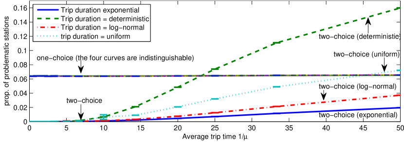
We simulate this model for four trip-time distributions (exponential, log-normal, uniform and deterministic). We plot in Figure 6 the proportion of problematic stations as a function of the average trip time, . In each case, the capacity of station is and the fleet size is equal to . We observe that, as expected, the performance for the two-choice model degrades as the trip time increases. This is explained by the delay in the information: when the trip time is large, a station that had few bikes available when the user departed does not necessarily still have few bikes when the user arrives. The performance of the original model is not affected by the variation of the average trip time, because the fleet size is equal to .
We compare the two models (one-choice and two-choice). For a very large average trip time, the performance when the two-choice rule is applied can even be worse than when it is not. Although counterintuitive, this phenomena can be explained by the delays: for example, let us consider that all trips have a duration of min. Then, a station that has few bikes available at time will have many users who decide to ride to it between time and time min. These users will not arrive before time min. As a consequence, it is likely this station will experience a burst of arrivals after time min, causing more problems than if the choices were made at random. As shown in Figure 6, this phenomena is exacerbated when the trip-time distribution is more concentrated (the proportion for problematic stations is increasing when going for deterministic to uniform to log-normal to exponential distribution).
We want to emphasize that this problem occurs only when the trip time is very large compared to the arrival rate (about when the distribution is log-normal). Hence, we conjecture that the problem would not occur in a realistic scenario. We plan to study this question in a future work.
6.3. Influence of Geometry on the Performance Metric
Our theoretical results and closed-form formula strongly rely on the assumption that the system has no geometry. In real-world systems, finding or returning a bike can induce a local search for an available bike or an available spot. Studying such systems analytically is out of reach. This section presents simulation results that show that the influence of geometry on the proportion of problematic station is limited, both for the basic model and the two-choice model. However, we show in Section 6.3.1 that it has an effect when other metrics are considered, such as the time to return a bike.
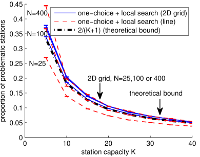
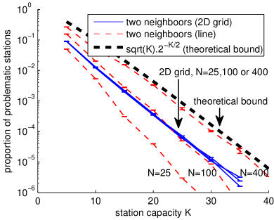
The model. We consider two representations of geometry represented in Figure 7 and 8: a 2D grid and a single line. The 2D grid is a schematic representation of a homogeneous city center like that of Manhattan. This situation aims at being a good representation of many bike-sharing systems: the stations are placed quite evenly on a plane and each station has a few neighbors (here, four) spread around it. The 1D line is a more extreme case that corresponds to a city spread along a single road. We expect the imbalances due to random choices to have more effect in the 1D line than in the 2D grid.
|
|
|
We simulate the two models. Users arrive at each station with rate . If the station is empty, the user leaves the system. Otherwise, she takes a bike. In the one-choice case (see Figure 7), she chooses a destination at random. If this station is saturated, she performs a random walk on the neighbors of the destination until she finds a non-saturated station. In the two-choice case (see Figure 8), the user chooses the least loaded station among two neighbors. Again, the user performs a local search if the station is saturated.
The proportion of problematic stations for all cases is reported in Figure 7 and Figure 8 for . In both cases, the models were simulated with , and stations. Each point represents the average over independent simulations. The error bars indicate confidence intervals but are most of the time too small to be seen. We compare these values with the theoretical bounds of the models without geometry: for the one-choice model (Figure 7) and for the two-choice model (Figure 8). In all cases, the performance exhibits the same trend in the models with geometry as the theoretical bounds. In particular, the performance obtained for the 2D grid are mostly independent of and are very similar to the theoretical bounds. This shows that the bounds obtained in Theorems 1 and 2 are representative of more realistic systems, even if they are obtained on models that do not take into account the geometry.
|
|
|
6.3.1. Average Number of Visited Stations
We now consider a different performance indicator that is the average number of stations that have to be visited before a bike can be returned. This metric is an indicator of how much time is necessary to return a bike. It is critical for users.
In the original model without geometry, this metric can be easily computed as a function of the proportion of saturated stations. Let be this proportion. With probability , the original destination is not saturated and the user visit only one station. Otherwise (with probability ) , the user chooses another destination at random and repeats this operation until she finds a non-saturated station. As the new destination is chosen at random, it also has a probability to be saturated. Hence, the number of visited stations before returning a bike is, on average, .
In our models with geometry (line or 2D grid), we consider that users perform a local search to return their bikes: if a destination is saturated, the user chooses one of the two (or four) neighbors and repeats the operation until she finds a available spot. This implies that the neighbors of a saturated station are likely to receive more bikes than stations not located nearby. Hence, the neighbors of a saturated station are more likely to be saturated than others. This creates local saturation and increase the average number of station that a user has to visit before being able to return her bike.
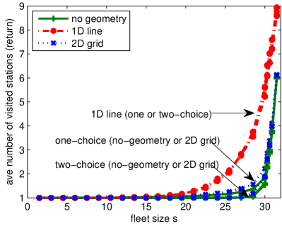
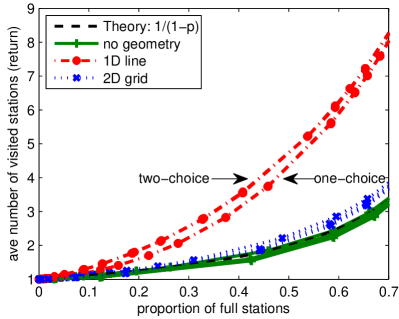
We simulate the three models and compute the average number of stations that a user visits before finding an available spot. The results are reported in Figure 9. In Figure 9(a), we plot the average number of visited stations as a function of the fleet size . This figure is to be compared with Figure 1 and Figure 10 for the one-choice case and with Figure 3 for the two-choice case. The capacity of the station is . When the number of bikes per station is low (fewer than ), there are almost no saturated stations. In this case, users successfully return their bike at their chosen destinations, most of the time. When the number of bikes is close to , we observe that the average number of visited stations rises quickly in the case of the line. In all cases, the results are plotted for the four trip-time distributions, but the curves are indistinguishable. For the 2D model, the average number of visited stations is slightly higher that than the non-geometrical case but remains similar.
To ease the comparison between the two metrics, we plot the average number of visited station as a function of the proportion of saturated station in Figure 9(b). As indicated before, when the new destination is chosen at random, the average number of visited stations is ; where is the proportion of saturated stations. We observe in Figure 9(b) that the 2D grid has a similar behavior as the non-geometric model. When the geometry is represented by a line, the number of visited stations is higher but it has the same order of magnitude. In particular, when percent or less of the stations are saturated, the average number of visited stations is lower than , and lower than twice the one without geometry. We remark that having percent of the stations that are saturated corresponds to an extreme situation222In our simulation, each station can host up to 30 bikes. Having more than percent of stations that are saturated occurs when there is a fleet of more than 25 bikes per station for the line and more than 30 bikes per stations for the 2D grid..
To conclude, our simulations show that a 2D grid exhibits a performance similarly to the theory. As the positioning of stations is similar to a 2D grid in many bike-sharing systems, this implies that the basic model reflects the behavior of realistic scenarios.
6.4. Adding Features to the Model (Search at Arrival, Shorter Search Time when Returning)
The features of the homogeneous model can also be changed, while keeping the model analytically tractable. For example, instead of leaving, a user who arrives at an empty station can visit randomly other stations to find a bike, consisting of attempts with exponential distribution with parameter . The loss of users or the avoidance of empty stations can be seen as the two extreme cases and . A similar modification can be done when returning a bike. The mean searching time for finding or returning a bike can also be different for the mean trip time .
These modifications do not change the nature of the model: the occupancy of station will still follow a geometric distribution. Only the influence of the fleet size will change. For example, if the reattempt times of a user who cannot return her bike at the first attempt, are exponentially distributed of parameter , then Equation (2) is replaced333 To see that, the proportion of bikes per station is the sum of two terms: the mean number of bikes per station and the mean number of users per station riding. This term is the product of the effective arrival rate times the mean riding time. The mean riding time is because it is the sum of the mean trip time and if the user returns at the -th attempt, i.e. with probability . It leads to the result. by
| (15) |
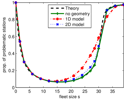
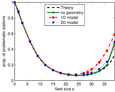
Moreover we simulate this model and report the proportion of problematic stations as a function of the fleet size per station in Figure 10. We plot the results for (Figure 10(a)) and (Figure 10(b)). In each case, we compare the theoretical prediction of Equation (15) with a simulation for and the two models with geometry presented in Section 6.3. We set and we vary and compare the four trip-time distribution (exponential, deterministic, log-normal and uniform). In all cases, the trip-time distribution has a negligible effect on the performance: for a given configuration, the relative difference between the proportions of problematic stations is at most . The geometry does have an effect, but the overall behavior is similar. As mentionned in Section 6.3, the performance of the 2D model is similar to the performance of a model without geometry.
6.5. Influence of Truck Capacity
In the redistribution model presented in Section 5, we assume that bikes are moved individually by a truck. This leads to a simple formula for the optimal redistribution rate. In practice, however, bikes are moved by trucks that can contain a few tens of bikes. This section reports simulation results of the model described in Section 6.3 where a truck of capacity is added. To obtain a fair comparison, the rate at which the truck visits the stations is set inversely proportional to the truck capacity. Hence, with this scaling, having a larger truck capacity leads to a poorer performance: the balance achieved when bikes are moved one by one at rate is better than when bikes are moved ten by ten at rate .
The simulated model is composed of stations that are placed in a 2D grid, as in Figure 7(a). Users move as in the one-choice model of Section 6.3: At each time step, a user arrives at one station picked at random, takes a bike if this station is not empty, and performs a local search if the targeted destination is saturated. At each time step, with probability , a truck transports bikes from the station that has the largest number of bikes and places them in the station that has the smallest number of bikes. The truck tries to equalize the number of bikes between the two stations but cannot move more than bikes at a time. The case corresponds to the model described before. The maximum number of bikes per time slot that can be moved by truck does not depend on and is equal to .
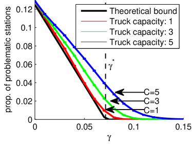
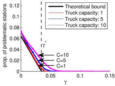
The proportion of problematic stations are reported in Figure 11 for two stations capacity: and . Recall . For , simulation results for , and are compared with the theoretical values obtained from the fixed point analysis. For , simulation results for , and are compared with the theoretical values. The vertical lines represent the optimal redistribution rate , obtained from Theorem 3. We observe that the theoretical model (with a truck capacity of one) predicts qualitatively the performance of the simulated models. This prediction is an optimistic estimation of the simulated values. Moreover, as expected, the performance decreases with the truck capacity.
To conclude, in an homogeneous system, the optimal redistribution rate depends on the capacity of the station and leads to a great improvement of the system performance. It can be shown that combining this redistribution mechanism with the two-choice incentives introduced in the previous section leads to an optimal redistribution rate close to .
7. Conclusion and Future Work
In this paper, we investigate the influence of the station capacities on the performance of homogeneous bike-sharing systems. Using a stochastic model and a fluid approximation, we provide analytical expressions for the performance. They are summarized in Table 1. The optimal fleet size is approximately for all models. Without using incentives, the capacity has only a linear effect on the performance or on the optimal redistribution rate. For this purpose, an incentive to return bikes to the least loaded station among two improves dramatically the performance, even if a small proportion of users accept to do this. Moreover, even if this model does not take into account any geographic aspect of the system, simulations show that these results also hold when considering simple geometric models with local interactions.
|
Optimal fleet size | |||
|---|---|---|---|---|
| Original model | ||||
| Two-choice | ||||
| Regulation | 0 if |
Our results prove that the effect of random choices on the performance should not be neglected when studying the performance of a bike-sharing system. Even in a completely balanced system, they dramatically affect the performance. A natural extension of this work is to consider stations with different parameters. The steady-state performance of such a system is given by [7]. It proves that, without repositioning via incentives or trucks, performance is very poor. One interesting question is whether the steady-state performance can be used as a metric in a system with varying operation conditions, such as peak-hours and non-peak hours. Our work can serve as a building block for studying the effect of incentives and redistribution mechanisms. Studying practical implementations of these mechanisms in real-world systems is postponed for future work. Moreover, the transient behavior of such mechanisms in a city where the attractiveness of stations varies over time could be studied.
References
- [1] P. Borgnat, P. Abry, P. Flandrin, C. Robardet, J.-B. Rouquier, and E. Fleury. Shared bicycles in a city: A signal processing and data analysis perspective. Advances in Complex Systems, 14(03):415–438, 2011.
- [2] D. Chemla, F. Meunier, and R. Wolfler Calvo. Bike sharing systems: Solving the static rebalancing problem. Discrete Optimization, 2012.
- [3] C. Contardo, C. Morency, and L.-M. Rousseau. Balancing a dynamic public bike-sharing system. Technical report, cirrelt, sept 2012. https://www.cirrelt.ca/DocumentsTravail/CIRRELT-2012-09.pdf.
- [4] P. DeMaio. Bike-sharing: Its History, Models of Provision, and Future. In Velo-city 2009 Conference. May, 2009.
- [5] P. DeMaio and J. Gifford. Will Smart Bikes Succeed as Public Transportation in the United States? Journal of Public Transportation, 7:1–16, 2004.
- [6] G. Fayolle and J.-M. Lasgouttes. Asymptotics and scalings for large product-form networks via the central limit theorem. Markov Process. Related Fields, 2(2):317–348, 1996.
- [7] C. Fricker, N. Gast, and A. Mohamed. Mean field analysis for inhomogeneous bike sharing systems. AofA 2012, International Meeting on Probabilistic, Combinatorial and Asymptotic Methods for the Analysis of Algorithms, 2012.
- [8] C. Fricker and N. Servel. Two-choice regulation in heterogeneous closed networks. Preprint, September 2013.
- [9] J. Froehlich, J. Neumann, and N. Oliver. Measuring the pulse of the city through shared bicycle programs. In International Workshop on Urban, Community, and Social Applications of Networked Sensing Systems - UrbanSense08, 2008.
- [10] N. Gast and B. Gaujal. Mean field limit of non-smooth systems and differential inclusions. ACM SIGMETRICS Performance Evaluation Review, 38(2):30–32, 2010.
- [11] N. Gast and B. Gaujal. Markov chains with discontinuous drifts have differential inclusion limits. Performance Evaluation, 2012.
- [12] D. K. George and C. H. Xia. Asymptotic analysis of closed queueing networks and its implications to achievable service levels. SIGMETRICS Performance Evaluation Review, 38(2):3–5, 2010.
- [13] D. K. George and C. H. Xia. Fleet-sizing and service availability for a vehicle rental system via closed queueing networks. European J. Oper. Res., 211(1):198–207, 2011.
- [14] G. A. Godfrey and W. B. Powell. An adaptive dynamic programming algorithm for dynamic fleet management, i: Single period travel times. Transportation Science, 36(1):21–39, 2002.
- [15] F. Guerriero, G. Miglionico, and F. Olivito. Revenue management policies for the truck rental industry. Transportation Research Part E: Logistics and Transportation Review, 48(1):202–214, 2012.
- [16] R. Katzev. Car sharing: A new approach to urban transportation problems. Analyses of Social Issues and Public Policy, 3(1):65–86, 2003.
- [17] T. Kurtz. Approximation of population processes. Society for Industrial Mathematics, 1981.
- [18] V. A. Malyshev and A. V. Yakovlev. Condensation in large closed Jackson networks. Ann. Appl. Probab., 6(1):92–115, 1996.
- [19] M. Mitzenmacher. The power of two choices in randomized load balancing. IEEE Transactions on Parallel and Distributed Systems, pages 1094–1104, 2001.
- [20] R. Nair and E. Miller-Hooks. Fleet management for vehicle sharing operations. Transportation Science, 45(4):524–540, 2011.
- [21] R. Nair, E. Miller-Hooks, R. C. Hampshire, and A. Bušić. Large-scale vehicle sharing systems: Analysis of vélib’. International Journal of Sustainable Transportation, 7(1):85–106, 2013.
- [22] T. Raviv and O. Kolka. Optimal inventory management of a bike-sharing station. IIE Transactions, (just-accepted), 2013.
- [23] T. Raviv, M. Tzur, and I. Forma. Static repositioning in a bike-sharing system: Models and solution approaches. Euro Journal of Transportation and Logistics, 2012. accepted for publication.
- [24] J. Schuijbroek, R. Hampshire, and W.-J. van Hoeve. Inventory rebalancing and vehicle routing in bike sharing systems. Technical report, Schuijbroek, february 2013.
- [25] S. Shaheen and A. Cohen. Growth in worldwide carsharing: an international comparison. Transportation Research Record: Journal of the Transportation Research Board, 1992(-1):81–89, 2007.
- [26] D. Tibi. Metastability in communications networks. arXiv:1002.07/96v1, 2011.
- [27] A. Waserhole and V. Jost. Vehicle sharing system pricing regulation: Transit optimization of intractable queuing network. Technical report, INRIA, 2012.
- [28] A. Waserhole, V. Jost, and N. Brauner. Pricing techniques for self regulation in vehicle sharing systems. Electronic Notes in Discrete Mathematics, 41:149–156, 2013.
