Can a Nanoflare Model of EUV Irradiances Describe the Heating of the Solar Corona?

Abstract

Nanoflares, the basic unit of impulsive energy release may produce much of the solar background emission. Extrapolation of the energy frequency distribution of observed microflares, which follows a power law to lower energies can give an estimation of the importance of nanoflares for heating the solar corona. If the power law index is greater than 2, then the nanoflare contribution is dominant.

We model time series of extreme ultraviolet emission radiance, as random flares with a power law exponent of the flare event distribution. The model is based on three key parameters, the flare rate, the flare duration and the power law exponent of the flare intensity frequency distribution. We use this model to simulate emission line radiance detected in 171 Å, observed by STEREO/EUVI and SDO/AIA. The Observed light curves are matched with simulated light curves using an Artificial Neural Network and parameter values are determined across regions of active region, quiet sun, and coronal hole. The damping rate of nanoflares is compared with radiative losses cooling time. The effect of background emission, data cadence, and network sensitivity on the key parameters of model is studied.

Most of the observed light curves have a power law exponent, $\alpha$, greater than the critical value 2. At these sites nanoflare heating could be significant.

1 Introduction

The mechanism of forming nanoflares is the dissipation of current sheets arisen from tangential discontinuities in the continuously evolving corona (Levine 1974, Parker 1988). Parker presumes that the change in the magnetic field across the current sheet, $\Delta B$, is critical for the onset. When the strength $|\Delta{B}|$ of the discontinuity exceeds some threshold, there is a runaway dynamical instability leading to an explosive reconnection phase. This is similar to the sand pile model that has been used to explain the comparison is also made between results of different methods. Avalanches of magnetic reconnection (Lu & Hamilton 1991), pointed out that the magnetic field of the corona is in a state of self organized criticality. To determine whether nanoflares are the main source of heat input to the corona or not, it is necessary to measure the energy frequency distribution of the smallest observed flares.

Hudson (1991) pointed out that the flare occurrence follows a power law distribution such as, $dN\sim E^{-\alpha}dE$, in which $dN$ is the number of flares per energy interval $E$ and $E+dE$ (Lu & Hamilton (1991) obtained this distribution for complex systems which are in a self organized critical state). The power law index, $\alpha$, is a critical value for determining whether more weight is given to small scale events (nanoflares) or larger ones (flares). Determination of the power law index of the flare frequency distribution is a scientific challenge. Many authors have attempted to find this index. Benz & Krucker (1998), using Yohkoh and SoHO, shown that the power law index at the microflare frequency distribution is 2.5. Parnell & Jupp (2000), used TRACE observations and concluded that the energy of nanoflares is insufficient to heat the quiet sun corona. Aschwanden & Parnell (2002) also get some other power law distribution by combining scaling law and fractal geometry for different observations. Aschwanden & Charbonneau (2002), gathered the statistics of solar flares, microflares, and nanoflares and concluded that, the power law index falls bellow the critical value. An extended review on the simulation and observational results is given by ( Klimchuk 2006 and Klimchuk et al. 2009).

To determine the contribution of small scale events (nanoflares) on the solar coronal heating, some applicable models has been investigated (e. g., Vekstein & Katsukawa 2000, Sakamoto et al. 2009, Terzo et al. 2011). Here, we use a model to simulate the observed Extreme Ultra Violet (EUV) emitted radiation from STEREO and SDO which has been applied successfully to the UV radiance fluctuation in the quiet Sun (Pauluhn & Solanki 2007) and later to SUMER observations of the corona in an active region (Bazarghan et al. 2008).

This paper is organized as follow: STEREO/EUVI and SDO/AIA data analysis are described in Section 2. The nanoflare model is treated in Section 3. A kind of Artificial Neural Networks (Probabilistic Neural Network) is briefly discussed in Section 4. In sections 5 and 6 the method and results are presented. The conclusions are given in Section 7.

2 STEREO/EUVI and SDO/AIA data analysis

STEREO (Solar TErrestrial RElation Observatory) is the mission in NASA‘s Solar Terrestrial Probes program (STP) which has been launched on October 2006 probes solar active phenomena and dynamics. It contains two identical observatories, one ahead (A) and the other behind (B) of the orbit of the Earth. Imaging the same events from two different locations enables us to have three dimensional images (http://stereo.gsfc.nasa.gov/).

Figure 1: (Left) The full disk STEREO/EUVI 171 Å image of the Sun and the three selected regions outlined with red boxes. This image has been recorded on 13 June 2007. (Right) The full disk SDO/AIA 171 Å  image of the Sun recorded on 22 August 2010.

The Extreme Ultra Violet Imager (EUVI) telescope is a part of SECCHI instrument suite which is sensitive at 171 Å, 195 Å, 284 Å, and 304 Å. In the present work we restrict ourselves to 171 Å images with time cadence of 2.5 minutes (Wüelser et al. 2004). The spatial pixel size of both A and B image is 1.6 arc second.

The SDO (Solar Dynamics Observatory) is designed to simultaneously study the solar atmosphere at small scales of space and time and in many wavelengths (http://sdo.gsfc.nasa.gov/
mission/instruments.php). It was launched on 11 February 2010.

The SDO/AIA provides full-disk imaging of the Sun in several UV and EUV bands with a pixel size of about 0.5 arcsecond and a cadence of 10 seconds.

Here, we take: (a) An STEREO/EUVI 171 Å  data set that has been recorded on 13 June 2007 with a cadence of 2.5 min, (b) SDO/AIA 171 Å data set that has been recorded on 22 August , 2010 with a cadence of 90 seconds.

The following steps are taken for data analysis:

-

Calibration of the recorded images using secchi$\_{\rm prep}$.pro on Solar Soft for EUVI data. The AIA level 1.5 data in the series, aia_test.synoptic2 are used. These are binned data with a pixel size of 2 arcsecond and a cadence of 90s.

-

To remove the solar differential rotation we use the Solar Soft routine derot$\_{\rm map}$.pro.

-

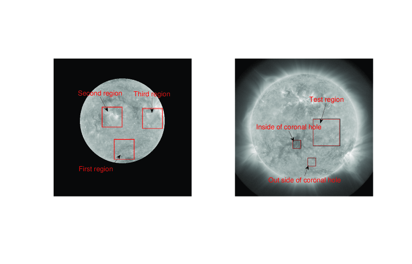
EUVI and AIA provide full disk images. We select three regions as shown in Figure 1 for EUVI data and two regions for the AIA data. It is attempted to select regions which cover active regions, quiet Sun and coronal hole. Consider the first selected region of EUVI images. We partitioned it into smaller $3\times 3$ pixels regions. Averaging on intensities of these smaller regions for $573$ success images, we obtain a light curve. The same process was followed for other small remained areas of selected region. In similar manner some other light curves were obtained too, while partitioning the selected region into $5\times 5$ and $9\times 9$ pixels regions. The above process was followed for other selected regions (on EUVI and AIA) too. We note that the light curves have 573 and 939 time steps for EUVI and AIA respectively. We fed each light curves (observed time series) to the network to determine the nanoflare model parameters (Section 6).

3 Nanoflare Model

Assuming that the coronal EUV emission is caused by many random flares with flare radiance, following a power law frequency distribution we take a model which consists of a time series of random kicks according to the presumption that flaring is intrinsically a stochastic process, each is given by a rising time $\tau_{r}$ and a damping time $\tau_{d}$ (Pauluhn & Solanki 2007, Safari et al. 2007, and Bazarghan et al. 2008). This model has five free parameters. The maximum and minimum flare amplitude, $y_{max}$ and $y_{min}$, the power law exponent $\alpha$, the damping time $\tau_{d}$ and the flare rate $p_{f}$. These are sufficient to produce our simulated EUV emission light curves.

Pauluhn & Solanki (2007) have shown that for a large number of independent random flares, the distribution of normalized radiance in quiet sun follows a lognormal. The same is true for active regions as pointed out by Safari et al. (2007) and Bazarghan et al.(2008).

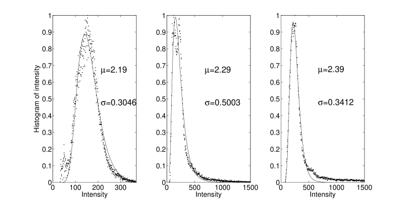
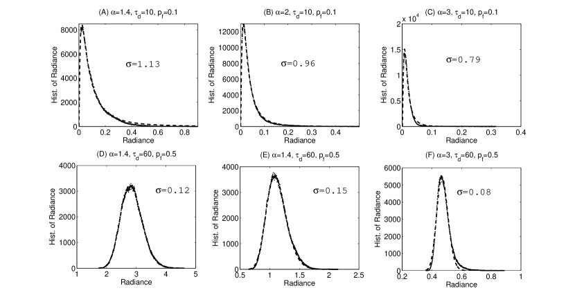
In the following, we focus on the distributions of three selected regions shown in Figure 1. The intensity distributions and the lognormal fits are shown in Figure 2. The lognormal function is given by

$$f(x,\mu,\sigma)=\frac{1}{x\sqrt{\pi\sigma}}\exp\left(-\left(\frac{\log x-\mu}{\sqrt{2}\sigma}\right)^{2}\right),$$ (1)

where, $x$, $\mu$, and $\sigma$ are the radiance, scale parameter, and shape parameter, respectively.

The good fits give us confidence in applying a stochastic flare model. The key parameters (power law exponents, damping rates and flare rates) of small scale events (small eruptions) are not identifiable directly from observations. Pauluhn & Solanki (2007) and Safari et al. (2007), estimated that the damping rates and flare rates could be deduced by comparing light curves with simulated time series. They have used the shape parameters of lognormal fits and wavelet analysis.

It is interesting to compare our model and it’s parameters to that of represented in recent works. Vekstein & Katsukawa (2000) assume that the energy distribution of the nanoflares has a power law spectrum, bounded between some minimum and maximum energy release. They suggest that: each nanoflares create a filament with cross-section area which has been then divided into small grids; nanoflares are generated randomly inside these grids with a finite occurrence rate; and evolves with two stage of cooling process (conduction and radiation heat). The heat conduction and radiation are derived according to scaling low (e. g., Rosner et al. 1978, Cargill 1993, Cargill & Klimchuk 1997). Sakamoto et al. (2009) have added the pressure balance (between internal gas and external magnetic field of elemental filaments) to this model and they analysed the SXT and TRACE intensities and intensities fluctuations. Terzo et al. (2011) introduce a constant heating as an intrinsically flat light curves and imposed the Poisson noise to simulate the light curves. They concluded that, the noises could not simulate the light curves observed Hinode/SXT. Performing a Monte Carlo simulation they perturb the flat light curves with a sequence of random segments of exponential decays linked together. The parameters of their model are the e-folding time, the interval between two successive perturbation and the amplitude. Finally they found some simulated light curves which is in best match with the observed data.

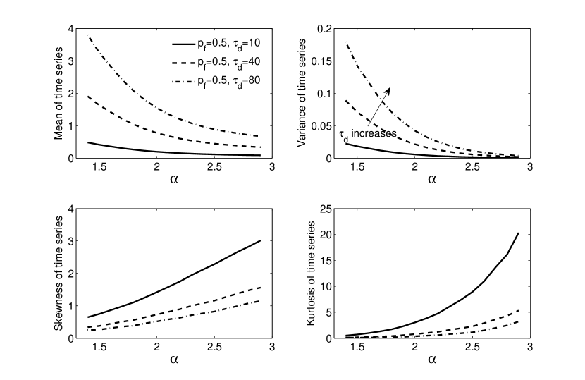
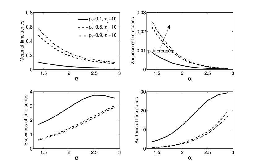
One may ask what happens to shape of the time series if the key parameters change. The light curves for flare models with different $\alpha$, $p_{f}$, and $\tau_{d}$ parameters are shown( Bazarghan et al. 2008, Figure 4). There is a physical picture of how the parameters affect the light curves. The mean, variance, skewness, and kurtosis of the time series are shown in Figures 3 and 4 versus $\alpha$. Both the mean and variance of the time series decrease, as $\alpha$ increases. Expectedly, the more the $\alpha$ (corresponds to more small events) the less the intensities become. With a fixed $\alpha$ and $p_{f}$ as $\tau_{d}$ increases, the mean and variance increases accordingly. This also occurs when $\alpha$ and $\tau_{d}$ are fixed and $p_{f}$ changes. The higher moments (skewness and kurtosis) of the time series increase with increasing $\alpha$, $\tau_{d}$, and $p_{f}$. Due to lognormal shape of the distributions, both skewness and kurtosis values are positive (Figure 5). A positive value of skewness signifies a distribution with an asymmetric tail extending out towards larger radiance. In general, the geometric median ($\exp(\mu)$) is less than the geometric mean ($\exp(\mu+\sigma^{2}/2)$). This is agree with Terzo et al. (2011). They have shown that, the distributions of intensity fluctuations taken from individual pixels, multi-pixel subregions, or the entire active region as observed by Hinode/SXT are asymmetric.

We knew that, the shape parameter is inversely in proportion to $\sqrt{\tau{p_{f}}}$ (Pauluhn & Solanki 2007) and that the lognormal shape parameter, $\sigma$, slightly changes with $\alpha$. Although, the sharpness of the distribution indicates that for a higher $\alpha$, the distribution shape tends to be sharpener as illustrated by the kurtosis increase (Figure 5).

Bazarghan et al. (2008) used Artificial Neural Networks (ANN) to compare SUMER/SoHO observational time series with simulated time series. In this paper, a similar method is employed to determine the three key parameters of SECCHI/EUVI and SDO/AIA time series. The main advantages of the ANN method is that it enables us to obtain quantitative values for all parameters including $\alpha$, with which Safari et al.(2007) had problem in analysis.

Figure 2: Left to right, the histogram of intensity for the first, second, and third selected regions and their own lognormal fits.

Figure 3: Mean, variance, skewness, and kurtosis of the light curves versus $\alpha$ for different $\tau_{d}$.

Figure 4: Mean, variance, skewness, and kurtosis of the time series versus $\alpha$ for different $p_{f}$.

Figure 5: Distribution functions of the simulated time series (dotted lines) and the best fit lognormal functions (dashed lines). The shape parameter varied considerably if $p_{f}\tau_{d}$ changed.

4 Probabilistic Neural Network

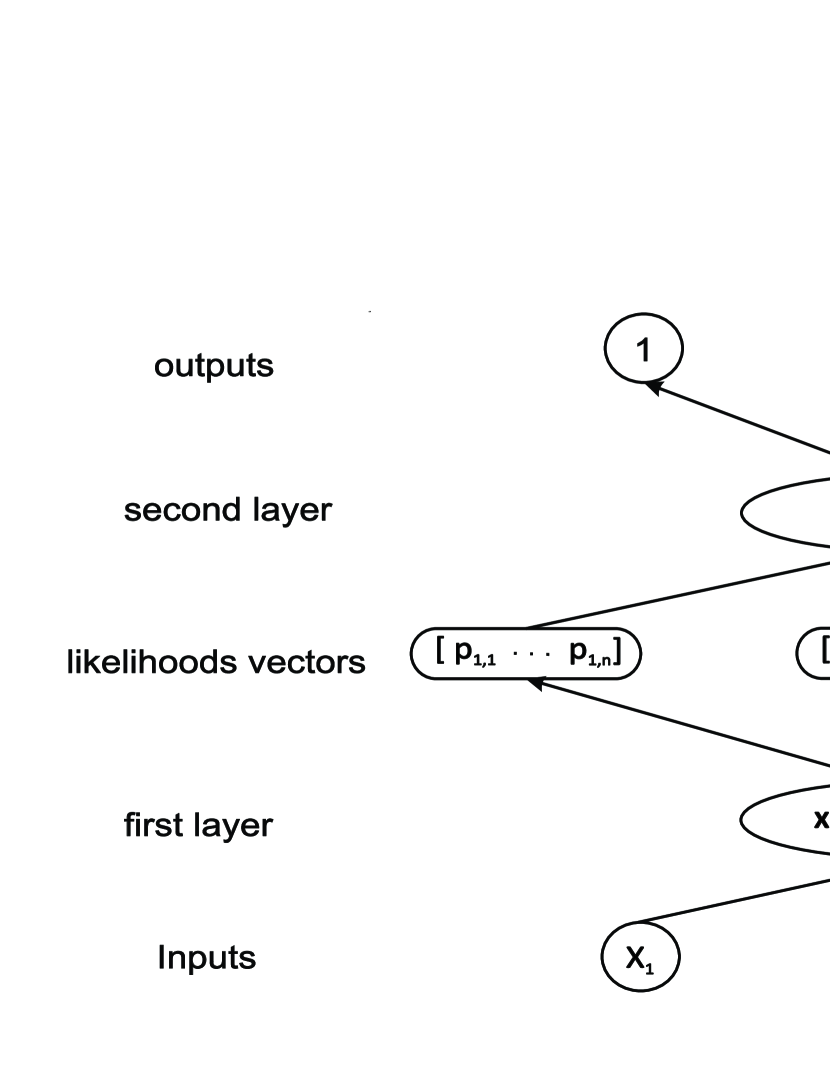
We employed a kind of Artificial Neural Networks, called Probabilistic Neural Network (PNNs Specht 1988, 1990) which is suitable for classification . A classification problem is defined with a set of inputs $P$ and targets $T$. PNN is a kind of supervised network. It means that the learning process of the network takes place with an initially specified set of inputs and targets, called trained samples. If we assume that the input vectors contain $k$ different classes, then every target vector would contains $k$ elements. One of them is 1, which corresponds to its own class and the others are zero. The PNN has two layers( Figure 6). When an input vector is fed to the network, the first layer calculates the distance between the input vector and the trained samples. So, it provides a vector the elements of which define the distance between the input and trained samples. The second layer produces a vector which contains the probabilities using the output of the first layer. Finally the competitive transfer function of the second layer chooses the maximum likelihood value within the probabilities vector and produces the output $1$ for it and the output zero for the others. Using this process, the network matches the input vector to one of the existing $k$ classes which has the maximum likelihood value.

We ran the commands of the mentioned process in the Neural Network Toolbox (Wasserman 1993).

Figure 6: The architecture of Probabilistic Neural Network

5 Methods

We employed the following steps:

1-

We ran the simulation code to generate the light curves. The power law exponent ranges between 1.4 $\leq\alpha\leq$4.4 in steps of 0.1; the duration time ranges between 2$\leq\tau_{d}\leq 80$ in steps of 1, the flare rate falls between 0.1$\leq p_{f}<$1 in steps of 0.1. A total amount of 22041 light curves for each combination of $\alpha$, $\tau_{d}$, and $p_{f}$ are obtained. For series with labels 1 and 7800 the set had ($\alpha=1.4$, $\tau_{d}=2$, $p_{f}=0.1$) and ($\alpha=2.4$, $\tau_{d}=8$, $p_{f}=0.6$), respectively. The larger the label’s value is, the greater the value of the power law index becomes.

2-

We fed the simulated light curves (as produced in previous steps) to the network. Now, the network was tested to see whether it has been well trained or not? A set of simulated light curves (trained samples) was selected (manually) to feed the network to enable it to recognize and classify. If the network was able to recognize then it would be trained. Since our model has been based on random number, we reproduced some light curves and fed them to the network for more accurate testing. We note that due to the network which uses a special function, the training error of the network is zero.

3-

The input weights of first layer of the network is a matrix, elements of which are the trained samples couples (input and targets). Let us consider an observed light curve which the set of it’s key parameters are not known. Once the unknown light curve (test sample) is fed to the network as an input vector, it’s distance from the 22041 trained vectors is calculated by the first layer. So, it would be determined how close the input is to the vector of trained set. Consequently, for an input vector closest to trained one, the existent transfer function of the first layer produces 1. If the input vector has the same distance from two or more trained samples, then the output includes two or more 1. The second layer weights are set to a matrix, elements of which are the target vectors. Each vector has only a 1 in the row associated with that particular class of input, and 0’s elsewhere. The output of first layer is multiplied by the matrix (target) and the product will be sent to the transfer function of second layer which produces 1 for the greatest existent value and 0’s elsewhere. Using these process, the network corresponds the input vector to one of the 22041 existent classes because that class had the maximum probability of being correct. The output of the classifier includes a number which labeled each classes, each corresponds to a set of key parameters. Now, the total observed light curves are fed to the classifier (network) as the test data set.

Figure 7: Left panel: The simulated light curves for three set of key parameters are shown as legends with $\tau_{r}/\tau_{d}=0.3$ and $y_{\rm max}/y_{\rm min}=100$. Right Panel: The observed light curves from EUVI 171 Å, for the first selected regions while averaging on intensities of the smaller regions ($3\times 3$, $5\times 5$, and $9\times 9$ pixels from above to bottom, respectively). Both left and right compared to each other using Artificial Neural Network.

Figure 8: Above panel: The frequency (histogram) of output labels (simulated light curves labels) for the observed light curves ( First region of STEREO/EUVI image) constructed by averaging on intensities of the smaller region ($3\times 3$ pixels). Bottom panel (from left to right): The histograms of $\alpha$, $\tau_{d}$, and $p_{f}$, respectively.

Figure 9: Above panel: The frequency (histogram) of output labels (simulated light curves labels) for the observed light curves ( First region of STEREO/EUVI image) constructed by averaging on intensities of the smaller region ($5\times 5$ pixels). Bottom panel (from left to right): The histograms of $\alpha$, $\tau_{d}$, and $p_{f}$, respectively.

Figure 10: Above panel: The frequency (histogram) of output labels (simulated light curves labels) for the observed light curves ( First region of STEREO/EUVI image) constructed by averaging on intensities of the smaller region ($9\times 9$ pixels). Bottom panel (from left to right): The histograms of $\alpha$, $\tau_{d}$, and $p_{f}$, respectively.

6 Results

6.1 Results for STEREO/EUVI

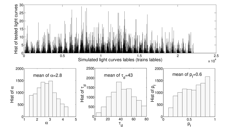
For each of the three selected regions (300$\times$300 pixels area) as marked on Figures 1, the light curves for average intensities were made. This gives, a set of 10000 light curves while averaging on the intensities of the smaller $3\times 3$ pixels regions, 3600 light curves while averaging on the intensities of smaller $5\times 5$ pixels regions, and 1089 light curves while the selected smaller regions are found to be $9\times 9$ pixels. These light curves were fed to the network. The network labeled each light curve with a set of individual key parameters which corresponds to a simulated light curve. The output result of the network is shown in Figures 7-10.

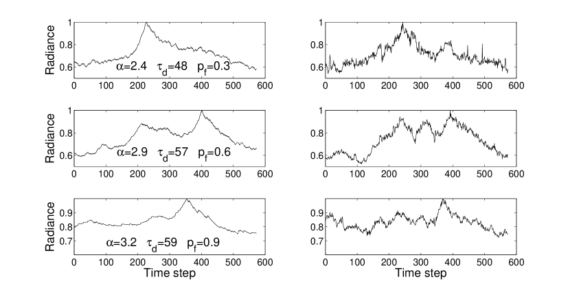
In Figure 7, the observed light curves are compared with their matched simulated light curves found by the network. We see that, the background radiance of the simulated light curves are remarkably close to the observed ones, which was a problem in previous studies of SUMER data (Bazarghan et al. 2008, see Figures 6 therein). As wee see, the observed light curves are noisier than the simulated one. One may wonder what would be the effect of the light curves’ noise on the network’s output? Using wavelet automatic de-noising (with different threshold and standard deviations) the noise of observed light curves is removed. In this case, the network’s output did not change.

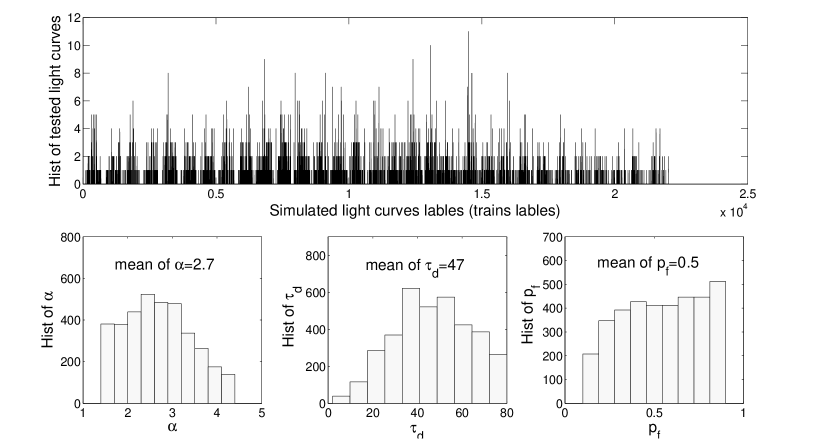
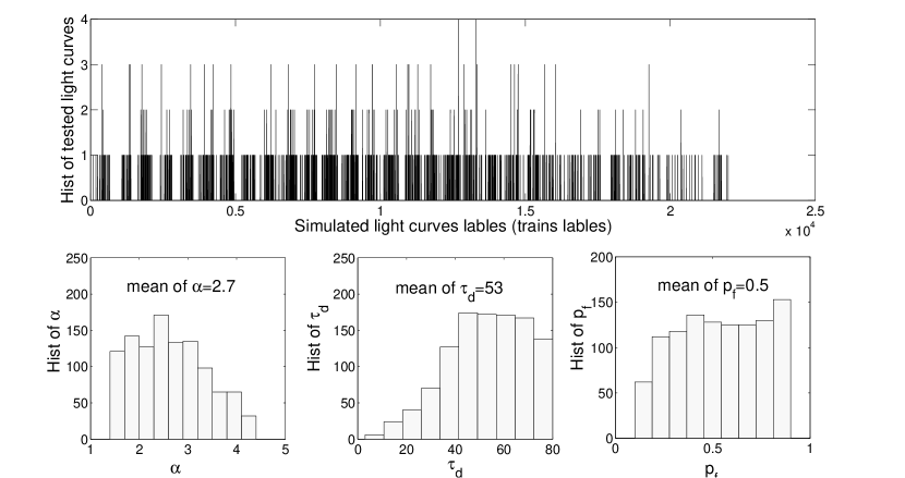
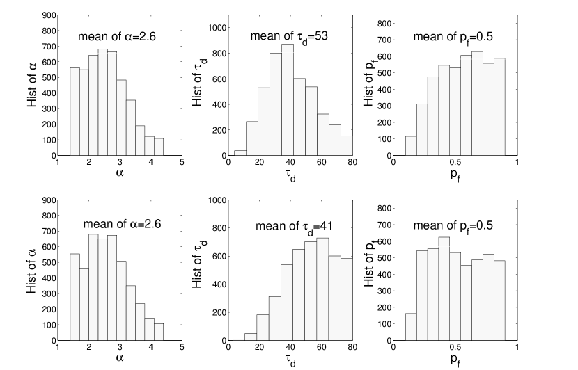
The frequency of the observed light curves (tested samples) versus simulated light curves (trained samples) is shown in the upper panels in Figures 8, 9, and 10. To do this, the histogram of output labels is calculated. We found that, these labels ranged from 1 to 22041, which corresponded to simulated light curves for which the key parameters range from the set of $(\alpha=1.4,\tau_{d}=2,p_{f}=0.1)$ to $(\alpha=4.4,\tau_{d}=80,p_{f}=0.9)$, as was stated in the previous section. In the bottom panels, the frequencies (histogram) of power law index, damping time, and flare rate, are extracted as well.

As we see in Figures 8, 9, and 10 the network’s output for $\alpha$ are concentrated on the range between 2-3. The mean power law index, $\alpha$, is 2.8, 2.7 and 2.6 for intensity averaged over $3\times 3$, $5\times 5$ and $9\times 9$ pixels, respectively. There are the similar values for the standard deviations, $\sigma\approx 0.7$. As was expected, the power law index falls as the the dimension of pixel’s average intensity increases. This confirms that, larger areas involve larger flare events. We note that the $\tau_{d}$ values increase with binning. For example, the average $\tau_{d}$ for $3\times 3$ pixels is 43 and for $9\times 9$ pixels it is 53. The $\tau_{d}$ seems to depend on the event size. This suggests that the larger areas as was expected have greater background.

The response of the STEREO/EUVI 171 Å  as a function of plasma temperature is within the range $\log T_{e}\approx 5.1-6.7$ (Wülser et al. 2004). If we suppose the plasma cooling through this narrow band filter is dominated by radiative losses process, then the cooling time, $\tau_{\rm cool}\approx\tau_{rad}$, would be ranged from a few seconds to an hour (see e. g., Aschwanden 2000, 2004). Using the mean dimensionless $\tau_{d}=43$ and multiplying it by cadence of 2.5 min (for STEREO/EUVI, 13 June 2007), we obtain a value of 2 hours. This is in good agreement with previous results (Aschwanden 2004).

Similar results are obtained for the two other selected regions. For the clarification of the background effects, we point at the SDO/AIA data in the following section.

6.2 Results for SDO/AIA

To explain the background effect on the three key parameters, $\alpha$, $\tau_{d}$, and $p_{f}$, we used SDO/AIA 171 Å  data sets taken on 22 August 2010. To do this, a region from inside and a region outside a coronal hole were selected (Figure 1, right panel). The time series with average intensity of $3\times 3$ pixels were constructed and fed to the network.

Figure 11: Above panel: The frequency (histogram) of output labels (simulated light curves labels) for the observed light curves (Inside of coronal hole of SDO/AIA image) constructed by averaging on intensities of the smaller region ($3\times 3$ pixels). Bottom panel (from left to right): The histograms of $\alpha$, $\tau_{d}$, and $p_{f}$, respectively.

Figure 12: Above panel: The frequency (histogram) of output labels (simulated light curves labels) for the observed light curves (Outside of coronal hole of SDO/AIA image) constructed by averaging on intensities of the smaller region ($3\times 3$ pixels). Bottom panel (from left to right): The histograms of $\alpha$, $\tau_{d}$, and $p_{f}$, respectively.

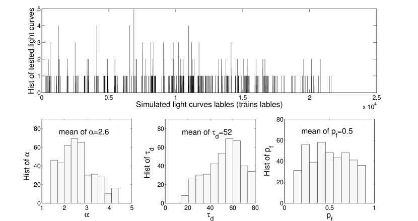
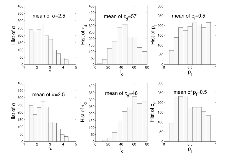
The outputs of the classifier network are shown in Figures 11 and 12. The average $\alpha$ for both regions are the same value (i.e., 2.7). We see that more than 73 percent of $\alpha$ with $\pm 1\sigma_{\alpha}$ (standard deviation $\sigma_{\alpha}=0.70$) falls about mean value. The average $\tau_{d}$ is 48 and 52 for inside and outside the coronal hole, respectively. There are 62 and 64 percent of $\tau_{d}$ with $\pm 1\sigma_{\tau_{d}}$ ($\approx$17) concentrated around mean values. This suggests that the background emission in the coronal hole is lower compared to its surrounding areas. One point is that there is no considerable difference between $\tau_{d}$ inside and outside the coronal hole. This is due to the fact that the damping times should be roughly the same everywhere because by choosing a specific filter we are picking up the same event phase. The average $p_{f}$ is 0.4 and 0.5 for inside and outside, respectively. Actually, more than 53 and 59 percent of $p_{f}$s with $\pm 1\sigma_{p_{f}}$ ($\approx$0.2) are concentrated around the mean values.

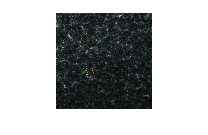
In the coronal hole the largest number of events have low flare rates $p_{f}\leq$0.2 (Figure 11). This is what one would expect when there is an almost low background as a consequence of open magnetic field. Outside the coronal hole, the average flare rate is $p_{f}=0.5$ (Figure 12). It seems that the higher the $p_{f}$ is, the smoother the background will be. As shown in Figure 13, this would explain why the higher $p_{f}$s are found in the cell centers (the bright regions of the mentioned Figure). The greater the variation of the background is, the lower the $p_{f}$ value will be. So, this explains why low $p_{f}$s are seen at the junctions (the dark regions in Figure 13).

The cadence of SDO/AIA (90s for 22 August 2010) is less than that of STEREO/EUVI (150s for 13 June 2007). As is shown in Figures 8 and 12 (we compare this figures because of their similar averaging dimensions on pixels regions) the higher the cadence is, the lower the average of damping time rate (which actually is less than 150/90) will be. For further examination, we produced AIA light curves with the cadences of $90$ and $180$s (for both regions partitioning $3\times 3$ and $5\times 5$ pixels) from the test region in Figure 1. Again the light curves were fed to the network and the frequency distribution of $\alpha$, $\tau_{d}$, and $p_{f}$, were shown in Figures 14 and 15. As we see, there is no change in average $\alpha$ and $p_{f}$ with changing cadences but the average $\tau_{d}$ decrease while the cadence is increasing.

Figure 13: The low $p_{f}=0.1$ events (red points) fall in the supergranul junctions (dark regions) and the high $p_{f}=0.9$ events (yellow points) fall in the supergranul cell centers (light regions). The image was cropped from the full disk image of SDO/AIA 1600 Å  22 August 2010.

Figure 14: frequency distribution of $\alpha$, $\tau_{d}$, and $p_{f}$ for the light curves of SDO/AIA (Figure 1, test region )with cadences of 90s (above panel) and 180s (bottom panel), which constructed by averaging on intensities of smaller region ($3\times 3$ pixels).

Figure 15: frequency distribution of $\alpha$, $\tau_{d}$, and $p_{f}$ for the light curves of SDO/AIA (Figure 1, test region )with cadences of 90s (above panel) and 180s (bottom panel), which constructed by averaging on intensities of smaller region ($5\times 5$ pixels).

7 Conclusions

The basic aim of the model, as mentioned earlier, is to determine the coronal heat input by numerous randomly distributed small scale events specially nanoflares by finding the power law index. This will decides whether the small scale event contribution is of importance or not. The problem of the too power law index indicated by researchers may have been just a bias due to neglecting the overlapping nanoflares.

Here, a simple nanoflare model based on three key parameters (the flare rate, the flare decay time, and the power law exponent of the flare energy frequency distribution) is used to simulate emission line radiances from the STEREO/EUVI and SDO/AIA in the corona. The simulation code ran to generate more than 22000 light curves (train set) for each combination of $\alpha$, $\tau_{d}$, and $p_{f}$. For each of the marked regions on the full solar disk images, more than 15000 light curves were generated for average intensities. This large number of perfect light curves which enable us in statistical description was focus of the present-paper. Light curve pattern recognition by a Probabilistic Neural Network (PNN) was employed to determine values of the key parameters. We found that more than 85% of the observed light curves have a power law index greater than 2. Since the network’s sensitivity depends on the training set in which the network must see all the possible patterns during the training session, we may have some errors in recognizing the correct patterns. Empirically, the network is sensitive to steps $\Delta\tau_{d}\approx 1$, $\Delta p_{f}\approx 0.1$, and $\Delta\alpha\approx 0.1$ for three key parameters. This means that, for shorter steps the light curves are too like, so that the network is not able to classify.

The results can be summarized as follows:

-

A physical picture of how the model’s parameters affect the simulated light curves is discussed. Decreases in both average and variance of the light curves are the function of increasing power law index (greater $\alpha$ value corresponds to greater number of small events). The higher moments (skewness and kurtosis) values of the time series are accompanied with increasing $\alpha$, $\tau_{d}$, and $p_{f}$ values (because of the lognormal shape of the distributions). Both the skewness and kurtosis values are positive numbers. The distributions of both simulated and observed light curves are asymmetric (Terzo et al. 2011).

-

The average $\alpha$ and $p_{f}$ did not change with changes in data cadences but the average $\tau_{d}$ is a sensitive function of decrease in cadence.

-

With regard to average dimensionless range of $\tau_{d}$=40-50s and by multiplying it by cadence of $2.5$ min (for STEREO/EUVI, 13 June 2007) and 1.5 min (for SDO/AIA, 22 August 2010) we obtain values of $100-125$ min and $100-75$ min, respectively. Assuming that plasma cooling through the narrow band filter is dominated by radiative cooling we find that the ranges are consistent with previous results.

-

The effect of the background emission on the flare rate, $p_{f}$ is studied. In the coronal hole regions with less background majority of events has low flare rates.

The next logical step is to determine the actual flare energies and the total energy input to the corona which is still a problem for researchers to be solved in the future.

References

- (1) Aschwanden, M.J., Alexander, D., Hurlburt, N., et al. 2000, ApJ 531, 1129
- (2) Aschwanden, M. J. & Parnell, C. E. 2002, ApJ, 572, 1048
- (3) Aschwanden, M. J. 2004, Physics of the Solar Corona, Springer: New York, p. 163
- (4) Bazargan, M., Safari, H., Innes, D. E., Karami, E., & Solanki, S. K. 2008, A&A, 492, L13
- (5) Benz, A. O. & Krucker, S. 1998, Sol. Phys, 182, 349
- (6) Benz, A. O. 2004, in: A. K. Dupree & A. O. Benz (eds.), Stars as Suns: Activity, Evolution, and Planets, Proc. IAU Symp. No. 219 (San fransisco: ASP), p.461
- (7) Cargill, P. J. 1993, Sol. Phys., 147, 263
- (8) Cargill, P. J., & Klimchuk, J. A. 1997, ApJ, 478, 799
- (9) Charbonneau, P. 2005, Living Review in Solar Physics, 2, 2.
- (10) Klimchuk, J. A. 2006, Solar Phys., 234, 41
- (11) Klimchuk, J. A.,van Driel-Gesztelyi, L., Schrijver, C. J., Merlose, D. B, Fletcher, L., Gopalswamy, N., Harrison, R. A., Mandrini, C. H., & Peter, H. 2009, IAUTA, 27, 79
- (12) Hudson , H. S. 1991, Sol. Phys., 133, 157
- (13) Levine, R. H. 1974, ApJ, 190, 457
- (14) Lu, E. T. & Hamilton, R. J. 1991, ApJ, 380, L89
- (15) Parnell, C. E. & Jupp, P. E. 2000, ApJ, 529, 554
- (16) Parker, E. N. 1988, ApJ, 330, 474
- (17) Pauluhn, A. & Solanki, S. K. 2007, A&A, 462, 311
- (18) Rosner, R., Tucker, W. H., & Vaiana, G. S. 1978, ApJ, 220, 643
- (19) Safari, H. Innes, D. E., Solanki, S. K., &Pauhluhn, A. 2007, in modern solar facilities - advanced solar science, 2006, Universitatsverlag Gottingen, ed. F. Kneer, K. G. Puschmann, & A. D. Wittmann, 359
- (20) Sakamoto, Y., Tsuneta, S., & Vekstein, G. 2008, ApJ, 689, 1421
- (21) Sakamoto, Y., Tsuneta, S., & Vekstein, G. 2009, ApJ, 703, 2118
- (22) Specht, D. F. 1988, in Proc. IEEE International Conference on Neural Networks, San Diego, CA, 1, 525
- (23) Specht, D. F. 1990, Neural Networks, 3, 109
- (24) Terzo, S., Reale, F., Miceli, M., Klimchuk, A., Kano, R., & Tsuneta, S. 2011, ApJ, 736, 111
- (25) Vekstein, G. & Katsukawa, Y. 2000, ApJ, 541, 1096
- (26) Wasserman, P.D., Advanced Methods in Neural Computing, New York, Van Nostrand Reinhold, 1993, 35.
- (27) Wülser, J. P., Lemen, J. R., Tarbell, T.D., et al. 2004, SPIE, 5171, 111