A new model for mixing by double-diffusive convection (semi-convection): I. The conditions for layer formation
Abstract
The process referred to as “semi-convection” in astrophysics and “double-diffusive convection in the diffusive regime” in Earth and planetary sciences, occurs in stellar and planetary interiors in regions which are stable according to the Ledoux criterion but unstable according to the Schwarzschild criterion. In this series of papers, we analyze the results of an extensive suite of 3D numerical simulations of the process, and ultimately propose a new 1D prescription for heat and compositional transport in this regime which can be used in stellar or planetary structure and evolution models. In a preliminary study of the phenomenon, Rosenblum et al. (2011) showed that, after saturation of the primary instability, a system can evolve in one of two possible ways: the induced turbulence either remains homogeneous, with very weak transport properties, or transitions into a thermo-compositional staircase where the transport rate is much larger (albeit still smaller than in standard convection).
In this paper, we show that this dichotomous behavior is a robust property of semi-convection across a wide region of parameter space. We propose a simple semi-analytical criterion to determine whether layer formation is expected or not, and at what rate it proceeds, as a function of the background stratification and of the diffusion parameters (viscosity, thermal diffusivity and compositional diffusivity) only. The theoretical criterion matches the outcome of our numerical simulations very adequately in the numerically accessible “planetary” parameter regime, and can easily be extrapolated to the stellar parameter regime.
Subsequent papers will address more specifically the question of quantifying transport in the layered case and in the non-layered case.
1 Introduction
1.1 The physics of semi-convection: double-diffusive convection
The concept of “semi-convection”, first introduced by Schwarzschild & Härm (1958), is often invoked in a number of rather different situations (Merryfield, 1995) which nevertheless have one point in common: they occur in regions which are stable to the Ledoux criterion, but unstable to the Schwarzschild criterion. Mathematically speaking, this condition can be expressed as
| (1) |
where , and are the temperature, gas pressure, and mean molecular weight, and where the subscript “ad” denotes a derivative at constant entropy. Physically speaking, (1) describes regions which are thermally unstably stratified, but where standard convection is suppressed by the presence of significant compositional gradients.
The first linear analysis of the stability of “semi-convective” regions was presented by Walin (1964) in the oceanographic context, and later by Kato (1966) in the astrophysical context. They both showed that a semi-convective region is hydrodynamically unstable, but to a much more gentle instability than the one associated with standard convection because it relies on doubly-diffusive processes to grow. It is in fact one of two forms of so-called “double-diffusive convection” (the other being fingering convection, otherwise known as “thermohaline convection” in astrophysics), and is often referred to as “double-diffusive convection in the diffusive regime” in physical oceanography. For the sake of clarity and brevity, we will refer to the phenomenon as “diffusive convection” in this series of papers.
As reviewed by Rosenblum et al. (2011), diffusive convection is principally controlled by three non-dimensional parameters. The first two characterize the nature of the fluid considered, and are the Prandtl number Pr and the diffusivity ratio ,
| (2) |
where , and are the viscosity, thermal diffusivity and compositional diffusivity respectively. For reference, note that Pr and are very roughly of the order of in giant planet interiors and in stellar interiors, and that is usually somewhat smaller than .
The third parameter is the inverse density ratio, defined as
| (3) |
which measures the relative importance of the destabilizing thermal stratification compared with the stabilizing compositional one. A semi-convective region is unstable (Walin, 1964; Kato, 1966) if
| (4) |
whereas regions with are unstable to overturning convection and those with are absolutely stable. Within this parameter range, it can be shown that the growth rate of the linear modes is complex. Furthermore, in the low Prandtl number regime characteristic of stellar and planetary interiors, the real part of the growth rate is proportional to the square root of the Prandtl number times the Brünt-Väisälä frequency (see Appendix A). In the same limit, the typical lengthscale of the unstable modes is a thermal diffusion scale.
Linear stability is unfortunately of rather limited utility, in particular when it comes to estimating the mixing rates induced by the diffusive convection. Experiments – laboratory or numerical – are the only way forward. Since no terrestrial fluid exists with similar values of Pr and , it is tempting to use experimental measurements of heat and compositional fluxes in different parameter regimes, in particular laboratory experiments in the heat-salt system relevant for physical oceanography (Linden & Shirtcliffe, 1978), and extrapolate them to the astrophysical case (Stevenson, 1982; Guillot et al., 2004). However one must be very cautious in doing so since the Prandtl number of water is typically 4-7, depending on temperature, whereas the Prandtl number in stellar and planetary interiors is much lower than one. Since the typical scale of the instability is a thermal diffusion scale, double-diffusive mixing is a mostly-laminar process at high Pr and a turbulent one at low Pr. There is no reason to expect that the laminar scalings should apply to the turbulent case.
Nevertheless, from a qualitative point of view, one of the most interesting results from laboratory (Turner & Stommel, 1964) and field experiments (Timmermans et al., 2008) in salt water is the fact that diffusive convection has a tendency to form thermohaline staircases, i.e. well-defined mixed layers separated by thin, very strongly stratified, and essentially diffusive interfaces. It is often thought that the necessarily weak transport through these interfaces is what controls and limits the efficiency of transport by “layered” convection. Such considerations have led Spruit (1992) and Chabrier & Baraffe (2007) for example to propose theories for heat and compositional transport in astrophysics, which rely on assumptions about the layer heights and the interface thicknesses. However, it is important to remember that, until very recently, layered convection had never been demonstrated to exist at low Prandtl number. As a result, these theories have, by and large, remained un-tested (see Rosenblum et al. (2011) for a review of prior numerical work).
1.2 Recent numerical and theoretical results
Recent 3D numerical simulations have finally shed some light on the subject of transport by diffusive convection. Rosenblum et al. (2011) ran an exhaustive numerical study of the phenomenon for fixed Prandtl number and diffusivity ratio Pr, and with the inverse density ratio spanning the entire instability range (4). While still far from any astrophysically-relevant regime, the selected values of Pr and in these simulations were below unity and therefore in the right “region” of parameter space. Rosenblum et al. (2011) found that the instability grows as expected and that the early behavior of the fluid can be satisfactorily explained by considering the fastest-growing modes of instability only. However, they discovered that two very different regimes of diffusive convection are possible after saturation of what we will refer to as the “primary” instability, depending on the value of the inverse density ratio. The various regimes are illustrated in Figure 1.
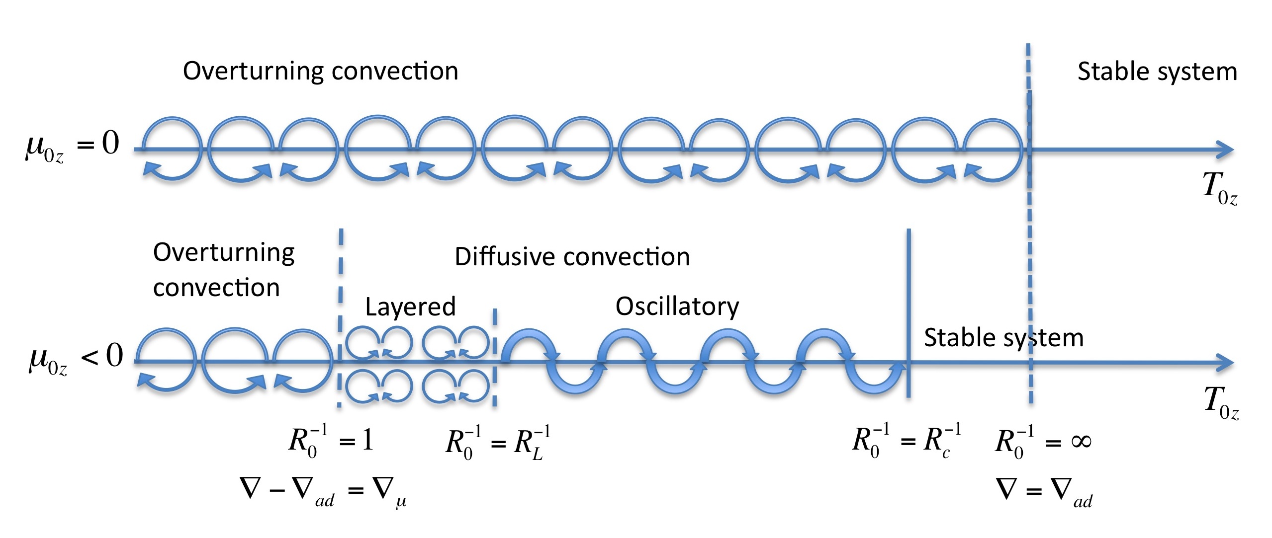
For large enough , i.e. for more “stable” stratifications, Rosenblum et al. (2011) showed that the system settles into a homogeneous, statistically stationary, weakly turbulent state. The turbulence is dominated by internal gravity waves111Recall that the background stratification is stably stratified in terms of the density and therefore supports standard gravity waves which oscillate with the buoyancy frequency. and mixing occurs principally via wave-breaking. Heat and compositional transport are fairly inefficient, and depend sensitively on the inverse density ratio. For low enough on the other hand, which corresponds to systems closer to the Ledoux-stability criterion, they observed the spontaneous emergence of thermo-compositional staircases after a short adjustment period. These staircases take the form of vigorously convective layers, which are thermally and compositionally well-mixed, and separated by fairly sharp interfaces, as observed in the oceanographic case. The interfaces, however, are far from merely diffusive and are instead very dynamic, and often pierced by strong localized updrafts and downdrafts. Later on, the layers are observed to merge, and each merger is accompanied by a significant increase in the overall transport across the staircase. Rosenblum et al. (2011) found that transport in that regime depends sensitively on the mean layer height, and proposed preliminary scalings to quantify it. The latter remain to be verified across a wider region of parameter space.
In fact, insight into the reason for this dichotomous “layered vs. non-layered” convection, can be gained from recent oceanographic studies of fingering convection, a related double-diffusive instability of thermally stable fluids which are destabilized by adverse compositional gradients (Stern, 1960). Such conditions are found in the tropical thermocline for example, where surface heating and evaporation continually warm up the upper layers of water, and increase its salt concentration. Crucially, thermohaline staircases are also commonly found in fingering regions of the ocean (Schmitt et al., 2005). Radko (2003) studied their formation in this regime, and showed that they can naturally emerge as a secondary large-scale “mean-field” instability of the system. More precisely, he showed that horizontally invariant but vertically sinusoidal density perturbations grow exponentially out of the homogeneous, small-scale fingering convection, and eventually overturn into a regularly-spaced staircase. His theory was later validated by Stellmach et al. (2011) via three-dimensional numerical simulations.
A crucial result of Radko’s theory is his identification of a necessary and sufficient condition for the layer-forming instability, namely that the turbulent flux ratio , defined as the ratio of the turbulent buoyancy flux due to heat transport, to the turbulent buoyancy flux due to salt transport, should be a decreasing function of the density ratio . He thus named the instability “the instability”. The fact that in salt water decreases with for low density ratios, then increases again for higher density ratios, explains why thermohaline staircases in the tropical ocean are only found in regions with low enough .
Recently, Rosenblum et al. (2011) showed that Radko’s instability theory can very easily and naturally be extended to explain the emergence of staircases in their own simulations of diffusive convection. The equivalent condition for instability is that the total flux ratio (i.e. the ratio of the total buoyancy fluxes, diffusive plus advective, of heat to composition respectively), should be a decreasing function of . Since the inverse density ratio is a more convenient parameter in diffusive convection, an equivalent sufficient condition for instability is that should be a decreasing function of . For completeness, the instability theory is rederived and discussed in Section 3. Rosenblum et al. (2011) found through their systematic exploration of the instability range that has a minimum at about when . This explains why layers are seen to form for in their simulations (at these values of Pr and ) but not for larger . Furthermore, in the simulations which do lead to layering, Rosenblum et al. (2011) found that theory and numerical experiments agree remarkably well on the growth rate of the instability. Their preliminary study thus suggested that, in order to know under which conditions layer formation is possible in stars and giant planets, one simply needs to determine if and when decreases with , for a given parameter pair .
1.3 Work outline
The findings of Rosenblum et al. (2011) lay a very clear path towards creating a practical model for transport by diffusive convection (semi-convection) in astrophysics:
-
1.
Model the function (from numerical simulations and/or theoretical calculations) to determine if and when layered convection is expected, and verify whether the -instability predictions continue to hold at lower and .
-
2.
Characterize transport by layered convection, and in particular, its dependence on layer height, , and .
-
3.
Characterize transport by homogeneous diffusive convection (i.e. in the absence of layers).
The first step is addressed in this paper, while steps 2 and 3 are deferred to subsequent publications in the series.
In the present paper, we therefore focus our efforts on a precise determination of the region of parameter space where layered convection is expected to occur. We do so using a combination of numerical simulations and theory. We discuss the numerical model and present typical results in Section 2. We review the instability theory in Section 3. In Section 4 we outline the methodology used for extracting the value of the flux ratio from simulations at numerically-accessible parameters, and present our results. In Section 5 we present a simple semi-analytical theory which enables us to estimate for any set of parameters, and compare it with our numerical results. In Section 6, we show that the predicted growth rates from the instability theory match the results of our numerical simulations very well. Finally, we conclude in Section 7.
2 Mathematical model and typical solutions
2.1 Mathematical model
As discussed by Rosenblum et al. (2011), the typical lengthscale of the fastest unstable modes is of the order of meters to hundreds of meters at most in the parameter regimes typical of stellar and planetary interiors. They found that the first layers to form are quite thin, spanning no more than a few of these fastest-growing wavelengths. This justifies studying diffusive convection (at least, in the early stages of layer formation and evolution), as a local rather than a global process.
We consider a local Cartesian domain of size , where gravity defines the vertical direction: . The small domain size permits the use of the Boussinesq approximation (Spiegel & Veronis, 1960) to the governing equations, which are then expressed as
| (5) |
The first of these equations is the continuity equation, where is the velocity field. The temperature and chemical composition fields (the latter is represented here for example as the mean molecular weight of the fluid) are expressed as the sum of a linear background profile ( and ) plus triply-periodic perturbations and . The thermal energy equation has been re-written as an advection-diffusion equation for , with being the thermal diffusivity. The additional term is present in compressible fluids but not in incompressible ones, and represents the temperature change due to adiabatic expansion (Spiegel & Veronis, 1960). Another advection-diffusion equation models the evolution of the mean-molecular weight perturbation , with the corresponding diffusivity. The last equation in (5) is the momentum equation; in the Boussinesq approximation, the density perturbation about hydrostatic equilibrium, , appears in the buoyancy term only, and is linearly related to the temperature and mean molecular weight perturbations as
| (6) |
where is the (constant) mean density of the region considered, and and are the coefficients of thermal expansion and compositional contraction respectively. The pressure perturbation is denoted as , and is the viscosity. All the perturbations satisfy triply-periodic boundary conditions,
| (7) |
where . This setup minimizes the effects of boundaries on the system.
Using the following standard non-dimensionalization (Rosenblum et al., 2011):
| (8) |
the governing equations can be re-written as
| (9) |
where quantities with tildes are dimensionless. The three parameters discussed in Section 1.1 naturally appear, namely the Prandtl number Pr, the diffusivity ratio , as well as the inverse density ratio , see equations (2) and (3). In the notations used here, we also have
| (10) |
It is interesting and important to note that this non-dimensional model now only knows about the superadiabatic temperature gradient rather than about and individually. As such, any two real physical systems with the same superadiabaticity, the same density ratio, and the same values of and , will lead to the same non-dimensional set of equations even if their background temperature gradients are different. This degeneracy in the parameters will be discussed in more detail in Section 3.
2.2 Typical results
Here we present the results of two selected simulations, which illustrate the behavior of diffusive convection in the planetary parameter regime. As mentioned in Section 1.2, previous work at Pr showed that the evolution of the system after saturation of the primary double-diffusive instability can either result in layer formation or not, depending on the value of the inverse density ratio . We confirm that this is still true at lower and . This is shown in Figure 2, which illustrates the two regimes for : the layered case, using (top row), and the non-layered case, using (bottom row). In each case, we show on the left a snapshot of the simulation at a particular time . On the right we show the temporal evolution of the non-dimensional thermal and compositional fluxes and , where denotes a spatial average over the entire computational domain.
In the case with low (top row), the basic instability rapidly saturates (around in non-dimensional time units), then transitions into a layered state, around . Three easily identifiable layers initially appear, which then merge into two (at about ) then one (at about ). The snapshot on the top left of Figure 2 was taken at , and shows the non-dimensional perturbation in the concentration field in the 2-layered state. The fluxes clearly increase in a stepwise manner, first when layers form and then at each merger. This kind of behavior was already illustrated and discussed by Rosenblum et al. (2011) (see their Figure 7).
In the case with high , the basic instability also grows (although more slowly, as expected from linear stability) and eventually saturates around . However, layers never form. Instead, what follows saturation is what Rosenblum et al. (2011) described as being a homogeneous, weakly convective phase with fairly inefficient transport properties. The snapshot on the bottom left of Figure 2 shows the non-dimensional perturbation in the concentration field at . Note the small amplitude of the perturbations, by comparison with the total compositional contrast across the domain ( here). Upon closer inspection, we find that the small-scale oscillatory structures that are characteristic of the homogeneous phase intermittently give way to somewhat larger-scale and more coherent gravity waves (e.g. here for and ; see also Figure 3). When this is the case the amplitude of the wave-induced oscillation in the fluxes dramatically increases, and the mean wave-induced transport also increases, although remains much lower than in the layered phase. The reason for the emergence of larger-scale waves and their self-organization remains to be determined, but the phenomenon is fairly ubiquitous at high (see below). This effect will be studied in a subsequent paper.
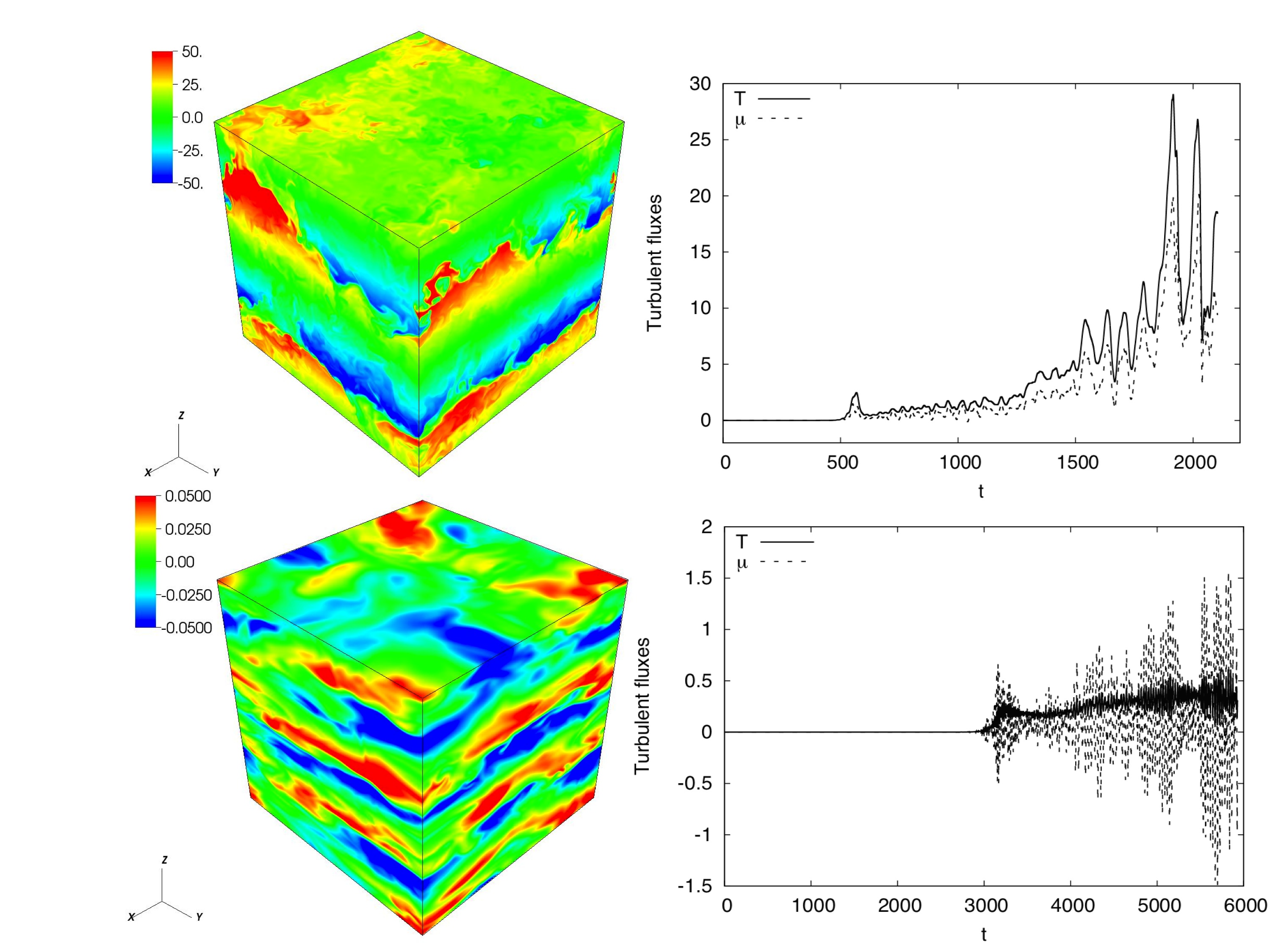
Figure 3 shows the evolution of the turbulent heat flux for parameter pairs ) with , for selected ranging from values close to overturning instability (left column), through intermediate values (middle column) to values close to marginal stability (right column). The plot clearly illustrates the following trends. Simulations with the lowest values of lead to very rapid layer formation, while those with slightly larger values of can stay in a state of homogeneous diffusive convection for a very long time before layers emerge (see the case of , for example). At intermediate values of , layers never form. The system remains in a state of homogeneous diffusive convection, and occasionally exhibits intermittent gravity-wave-dominated phases similar to the one described earlier. Finally, in runs with larger values of closer to marginally stability we always see that the wave-dominated phase begins very quickly after saturation of the primary instability. These various types of behavior need to be kept in mind when analyzing the data to extract their mean transport properties, as described in Section 4.

3 The instability revisited for case
In this Section we rederive the instability theory for the sake of completeness, and to correct a slight inconsistency in nomenclature discovered in the work of Rosenblum et al. (2011). While their derivation is technically correct222See associated Erratum for correction of a typo., it requires a slight physical re-interpretation of the quantities they define as “thermal Nusselt number” and “total buoyancy flux ratio” in order to be fully consistent when , as shown below.
The instability theory, first proposed by Radko (2003) in the context of fingering convection in the ocean, is a mean-field theory that describes the development of secondary instabilities in fully-developed double-diffusive convection (the theory is in fact valid both in the diffusive regime and in the fingering regime). The theory assumes that the system is already in a homogeneous and quasi-steady turbulent state and studies its evolution when subject to perturbations on scales much larger than the turbulent eddies. Accordingly, we begin by averaging the governing non-dimensional equations (9) over all small lengthscales and fast timescales, and study the evolution of the large-scale, more slowly evolving mean fields.
An emerging staircase is a horizontally invariant structure with no mean flow. If we ignore the momentum equation, and neglect mean flows as well as horizontal derivatives, the averaged non-dimensional thermal and compositional advection-diffusion equations become:
| (11) |
where denotes a spatio-temporal average over small-scales and short timescales. Note that the vertical fluxes and include a diffusive and a turbulent component. The goal is to express them in terms of large-scale fields only and thus close the system of equations, so that the latter can be solved for the evolution of and .
It is important to note for the upcoming discussion that there is, at this point, some degree of flexibility in the definition of these two fluxes: one can add or subtract any constant to and without changing the expression . In the original derivation of the instability, the fluxes are thus taken to be the total non-dimensional heat and compositional fluxes through the system, including the diffusion of the background fields and . When expressed non-dimensionally,
where the subscript denotes a derivative with respect to .
However, while the definition of as a total heat flux is intuitive and perfectly adequate for incompressible fluids (for which the theory was originally designed), a subtle but crucial problem emerges for compressible systems, where . The total heat flux explicitly depends on , while the original system of equations (9) only knows about , as discussed in Section 2.1. This remark suggests that the dynamically relevant quantity is instead
| (12) |
The flux thus defined, however, is no longer the total heat flux except when . Simplifying the resulting expressions for and yields
| (13) |
These expressions are the ones actually used by Rosenblum et al. (2011). The system of equations (11) and (13) are now mathematically consistent333An alternative, but equivalent, way to resolve the problem discussed here is to introduce the “potential temperature” commonly used in the atmospheric literature (e.g. Holton (1992)). The evolution equation for is identical to that for , except that the adiabatic gradient of is zero by construction. mean-field versions of the original system (9).
We now define two non-dimensional quantities:
| (14) |
The first, , reduces to the much more commonly used temperature thermal Nusselt number (i.e. the ratio of the total heat flux to the diffused heat flux) when . In what follows, we call it the “thermal Nusselt number proxy”. We also refer to the second, , as the “flux ratio”, for simplicity. When , it reduces to the total buoyancy flux ratio commonly used in physical oceanography.
The theory then continues exactly as in Rosenblum et al. (2011), by assuming that and each depend only on the fluid parameters and and on the local inverse density ratio. The latter can vary with as a result of the large-scale background temperature and compositional perturbations and , as
| (15) |
where, for clarity, we first expressed as the ratio of dimensional quantities and then as the ratio of non-dimensional quantities.
Combining (11), (14) and (15) yields a nonlinear system of equations describing the spatio-temporal evolution of the large-scale fields:
| (16) |
If and are known, finite, non-zero, and smooth enough, then the system of equations is closed and well-posed. It has a trivial steady-state solution when and are constant. This solution corresponds to a homogeneously, diffusively convective state with constant density ratio . Without loss of generality, we can choose our reference state and to be that steady-state solution, in which case , and . The flux ratio and thermal Nusselt number proxy of the homogeneous background turbulent state are noted as and .
Solving (16) in the general case is numerically possible if the functions and are known, but not particularly informative. However, we can linearize the mean-field equations around the previously defined homogeneously convective state, assuming that the large-scale perturbations and have small amplitudes. To linear order, the local inverse density ratio becomes
| (17) |
Noting that depends on via , it can be shown using the chain rule that, to linear order, the temperature equation becomes
| (18) |
where
| (19) |
while the linearized composition equation is similarly derived to be
| (20) |
where
| (21) |
Assuming normal modes of the form , we finally get
| (22) |
This quadratic recovers the one obtained by Radko (2003) and Rosenblum et al. (2011) exactly, the only difference being in the physical interpretation of the quantities and , as discussed above, when .
As originally discussed by Radko (2003), inspection of (22) shows that the condition for the existence of growing solutions is that the constant term in the quadratic should be negative, which only occurs when is positive, i.e., when is a decreasing function of . In the diffusive case studied here, one can prove by inspection of the sign of the linear term in (22) that this sufficient condition is also a necessary condition for instability (by showing that even if there are complex conjugate roots to this equation, their real parts are negative). Radko (2003) also showed that the instability theory suffers from an ultraviolet catastrophe whereby the mode growth rate is proportional to (so that modes with the smallest wavelengths always grow most rapidly). The theory, however, must break down when the layering mode wavelength becomes comparable with the basic instability wavelength. As a result, the actual mode which ends up growing out of the homogeneous turbulence is the one with the smallest wavelength for which the mean-field theory is still valid. Empirically, we find that the latter typically has a vertical wavelength that is about 2-4 times larger than the horizontal wavelength of the fastest growing mode of the basic instability according to linear theory (see Appendix A). In other words, the staircase typically forms with an initial step separation of about 25-50.
Finally, in order to identify more quantitatively the conditions for instability and predict its growth rate, we must measure the turbulent fluxes in the homogeneous phase of diffusive convection to estimate , , and , for various values of , and . In all that follows, we therefore limit our definitions of and to the case where , and so
| (23) |
We also define for convenience a compositional Nusselt number
| (24) |
which measures the ratio of the total compositional flux to the diffused compositional flux in the homogeneous phase. With this definition,
| (25) |
4 Measurements of the flux ratio
As we have just shown in Section 3, double-diffusive layering is expected to occur spontaneously whenever the flux ratio defined in (23) is a decreasing function of the inverse density ratio . In what follows, we refer to the function as “the curve”. In order to establish when the curve decreases and estimate the -instability growth rate, we now perform a series of numerical experiments, decreasing Pr and down progressively towards the astrophysically relevant parameter regime, and measure both and for the whole range of density ratios unstable to diffusive convection (see (4)). Section 4.1 describes our experimental setup and the manner in which we extract the flux ratio and the Nusselt numbers from the simulations. Section 4.2 presents and discusses our results.
4.1 Experimental setup
As in Rosenblum et al. (2011) and Traxler et al. (2011a), we use a computational box of size , which is about 4-6 times the wavelength of the fastest-growing mode of instability, regardless of the parameters selected (see Appendix A). This domain size was found to be sufficiently large to yield statistically meaningful measurements of the turbulent fluxes while remaining computationally tractable in the increasingly extreme parameter regimes studied.
We consider four values of Pr and , equal to 0.3, 0.1, 0.03 and 0.01 respectively. The two smallest values, 0.03 and 0.01, are within the planetary parameter range. For each (Pr,) pair, we run a number of simulations varying , selecting preferentially values close to one to capture the expected decreasing part of the -curve. Since the code is a Direct Numerical Simulation with no sub-grid model, each numerical experiment has to be fully resolved on all scales. Prior to each full-scale run, we test various resolutions and select the most appropriate one based on inspection of the vorticity, velocity and chemical composition field profiles and spectra. Runs with close to unity require the highest spatial resolution while runs with close to marginal stability require lower spatial resolution, but much higher temporal resolution and longer integration times to follow simultaneously the buoyancy frequency timescale and the much slower instability growth and saturation timescales. Tables 1 and 2 summarize the parameters selected and resolution for all our simulations.
| Pr | layers? | ||||
| Y | |||||
| Y | |||||
| Y | |||||
| Y | |||||
| ? | |||||
| N | |||||
| N | |||||
| N | |||||
| Y | |||||
| Y | |||||
| Y | |||||
| ? | |||||
| N | |||||
| N | |||||
| N | |||||
| N | |||||
| Y | |||||
| ? | |||||
| ? | |||||
| N | |||||
| N | |||||
| N | |||||
| N | |||||
| Y | |||||
| ? | |||||
| ? | |||||
| N | |||||
| N | |||||
| N |
| Pr | layers? | ||||
| Y | |||||
| Y | |||||
| Y | |||||
| ? | |||||
| N | |||||
| N | |||||
| Y | |||||
| Y | |||||
| ? | |||||
| N | |||||
| N | |||||
| Y | |||||
| Y | |||||
| Y | |||||
| ? | |||||
| N | |||||
| Y | |||||
| Y | |||||
| ? | |||||
| N | |||||
| N |
For each simulation, the PADDI code returns the non-dimensional instantaneous fluxes integrated over the entire computational domain as diagnostics of the simulations. However, the thermal Nusselt number proxy and flux ratio defined in the derivation of the instability theory (see Section 3) are only meaningful when viewed as temporal averages taken during a time where the system is in the assumed homogeneous, quasi-steady, diffusively convective state. Identifying that state, unfortunately, turns out to be significantly more difficult than expected. Figure 3 shows that transport in diffusive convection is much more variable than in the related fingering regime, where the layering theory and the methods for extracting small-scale fluxes were first derived (Traxler et al., 2011a). The underlying reason for this difference actually remains to be determined. Our selected domain size, for example, was initially chosen by analogy with studies of transport in fingering convection by Traxler et al. (2011a) and Traxler et al. (2011b), where it was found to be “[…] small enough to suppress any secondary large-scale instabilities” (Traxler et al., 2011a). We find here, by contrast, that large-scale perturbations (layers, large-scale gravity waves) do in fact grow even in such a small domain, and cause the observed variability in the fluxes.
In Appendix B, we discuss the problem in detail, and propose a systematic method to identify the homogeneous state described above, and extract the fluxes, Nusselt numbers and flux ratio in that phase. The results are presented below.
4.2 Nusselt numbers and flux ratio
Our measurements for and and , obtained using the method described in Appendix B, are summarized in Figures 4 and 5 respectively for each parameter pair (). The full dataset is presented in Appendix B.
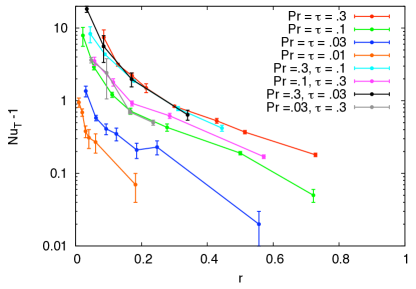
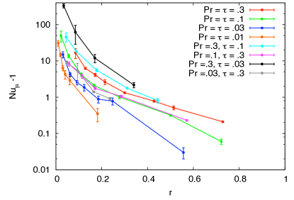
Figures 4a and 4b show and respectively. Each curve represents one parameter pair , and is plotted against the stratification parameter , where
| (26) |
This quantity is introduced, following Traxler et al. (2011b), to re-map the instability range into the interval , with corresponding to Ledoux criterion ( being unstable to overturning convection) and corresponding to the marginal stability limit ( being fully stable). This new variable eases the comparison between the various datasets, and can be interpreted as a rescaled bifurcation parameter which measures the distance to stability/overturning instability.
Figure 4 is reminiscent of a similar figure obtained by Traxler et al. (2011b) in the fingering regime. The thermal Nusselt number proxy is of the order of a few tens, and the compositional Nusselt number is of the order of a few hundreds for systems which are nearly Ledoux-unstable. Both rapidly drop to one close to the marginal stability limit (, . Since a real Nusselt number can also be viewed (in the Boussinesq limit) as the ratio of the effective diffusivity (turbulent + microscopic) to the microscopic diffusivity, with
| (27) |
our results show that turbulent compositional transport can be significant for more unstable systems. An equivalent interpretation for heat transport is more delicate, since can only be viewed as a Nusselt number when .
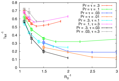
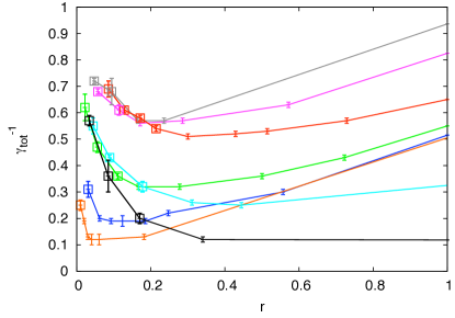
Figures 5a and 5b show the flux ratio measured in the simulations, as a function of and as a function of respectively. Both figures reveal many interesting features. We find that for all explored, there exists a region where decreases with (equivalently, with ), hence, where layer formation is possible according to the instability theory. We can therefore immediately compare our theoretical expectations with the actual outcome of the simulations: Figure 5a and 5b show runs which lead to layer formation as larger symbols. For larger values of Pr and (i.e. Pr, equal to 0.3 or 0.1), we confirm that layers indeed form whenever is a decreasing function of , hence validating the adequacy of Radko’s criterion. For lower Pr and , computational constraints limit our ability to validate Radko’s theory as systematically as in the higher Pr and case. Indeed, the layering mode growth rate depends on the derivative of (see Section 3), so the emergence of layers can be delayed significantly in runs with values of close to the minimum of the curve (see for example Figure 3 for , ). Since simulations at lower values of Pr and require considerable spatial resolution, we were not always able to integrate them for enough time to see the emergence of layers. We have seen them for very low values of where the curve decreases most rapidly, and expect that they should appear for slightly higher values of as well.
The fact that layering is possible in diffusive convection at low and is in stark contrast with results from the fingering regime (Traxler et al., 2011b), where always seems to increase with in the same limit. This rather remarkable difference in behavior is actually fairly easy to understand. Indeed, let us first look at the behavior of the curve close to marginal stability. In the corresponding runs, turbulent transport becomes negligible (see Figure 4), so the flux ratio is dominated by diffusive transport. Mathematically speaking,
| (28) |
which explains the observed oblique asymptote up to the limiting diffusive value at (see Figure 5b). In the diffusive regime considered here, is always smaller than one. However a similar argument applies in the fingering regime and yields . This limit “pulls up” the end of the curve to very large values, effectively preventing the existence of a region where decreases with .
5 Theoretical predictions for the flux ratio
The numerical simulations we have been able to perform sample parameter space reasonably comprehensively for and between 0.01 and 0.3, in particular for values of close to unity. We found that for all parameter pairs studied, there exists a interval where the function decreases, and that spontaneous layer formation indeed occurs in that region as expected from the instability theory. However, in order to create a model for diffusive (semi-) convection that can be used practically and efficiently in a planetary or stellar evolution code, it would be preferable to have an analytical or semi-analytical theory for the position of the minimum of the curve, rather than having to rely on interpolations or extrapolations of the available dataset presented in Tables 6 and 7. In this section, we propose such a model.
5.1 Theoretical model for
While we are looking for a model of the flux ratio , it is interesting to note that a method for estimating the turbulent flux ratio
| (29) |
from linear theory was first proposed by Schmitt (1979) in the context of fingering convection. Schmitt’s theory adequately captures the shape of the curve measured from laboratory (Schmitt, 1979) and numerical experiments (Traxler et al., 2011b), and in particular its dependence on Pr and , although the exact value of for a given value of could be off by 20-40%. As such, it should be considered as a qualitatively accurate indicator of scalings and trends, but is quantitatively reliable only within factors of “a few”.
Schmitt’s method can straightforwardly be applied to diffusive convection, as derived in Appendix A3. The resulting expression for is given by equation (A13), and depends on the growth rate and wavenumber of the most rapidly growing mode according to linear theory at the selected parameters , Pr and . The latter can be found numerically quite easily by solving simultaneously a cubic and a quadratic equation. If is known, then
| (30) |
where we have used equation (23) to express the turbulent heat flux in terms of . All that remains to do is to create a model for as a function of the system parameters , Pr and .
We now return to the results of the numerical simulations presented in Section 4.2. We find that we can satisfactorily fit the behavior of for large values of provided . Close to overturning instability, on the other hand, we find that a first satisfactory fit to the data has . This functional dependence is not unexpected, since is the non-dimensional background density gradient, and since diffusive convection relies on to operate, and is much more efficient the smaller the value of . Combining this fit with the large limit suggests a functional form with . One can fit the proportionality constant for runs with Pr = , and obtain a rather good match to the data. However, the resulting expression is less satisfactory for Pr . Further investigation reveals that an even better fit can be obtained with
| (31) |
The large uncertainty on the power index of the term comes from the uncertainty on the measurements themselves, compounded with the short range of Pr/ values available. However, its exact value does not matter much for the predictions.
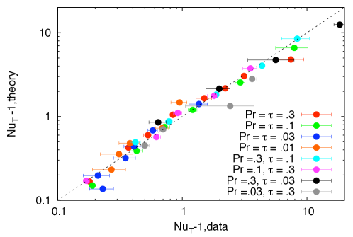
Figure 6 compares our empirical fit for given by equation (31) to the actual data. This fit is satisfactory for our current purposes, although we recognize that a better theoretically-motivated one should be sought in the future if we wish to improve on the model further.
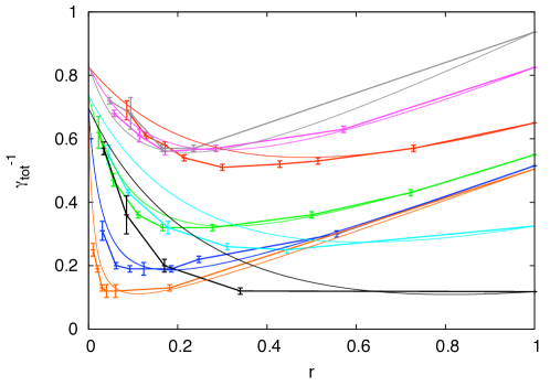
Using (A13), (30) and (31) we can now estimate semi-analytically. Figure 7 compares our predictions with the data presented in Figure 5b. As expected from the limitations of Schmitt’s method, and uncertainties in our fit for the turbulent heat flux, the model does not match the data perfectly. Generally speaking, we find that the predicted value of at the minimum is somewhat overestimated by the model, by 20-40%. The slope of the curve is thus also affected. These discrepancies are larger and/or more apparent for runs with larger values of the Prandtl number, for which the position of the minimum occurs for larger values of . However, it is nevertheless rather remarkable to see how well our model accounts for the shape of the curve, and in particular the variation of the position of the minimum with Pr and . The value of at the minimum is also robustly predicted by the model.
5.2 Model trends
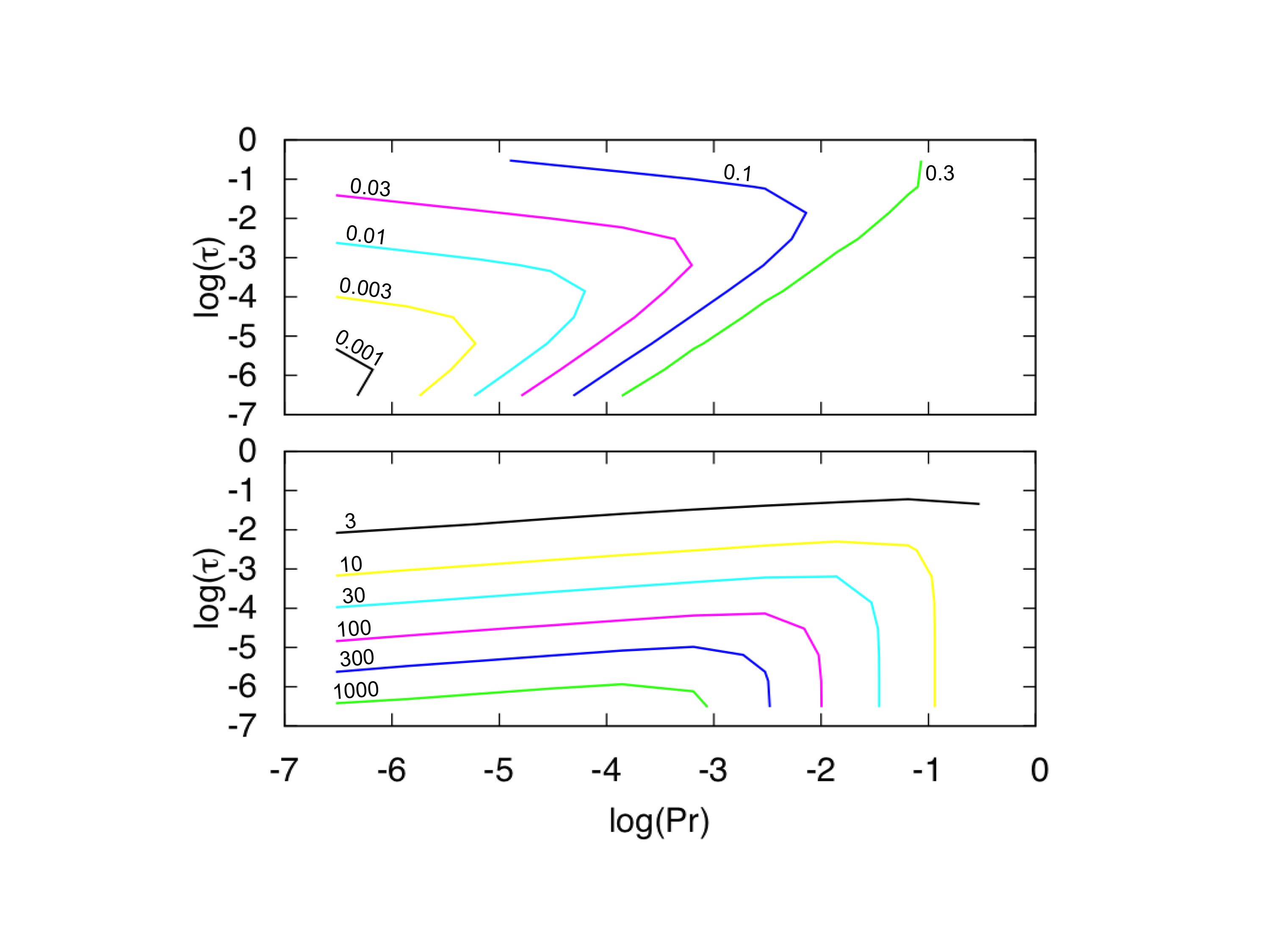
Using the model described in the previous section, we can now estimate the value of the inverse density ratio for which is minimal, for a range of parameter values beyond those for which we were able to run numerical simulations. The results are presented in Figure 8, for Pr and varying from to 1, and show contour plots of (bottom) and of the corresponding (top). Note that both and estimated directly from the model, as shown here, are likely to overestimate the true position of the minimum by about 20%-40% (see previous section).
Overall we find that the relative fraction of the total instability range unstable to layering decreases as Pr and decrease (i.e. the value of at the minimum of the curve decreases). However, since the instability range itself increases as Pr and tend to zero, the value below which layers can spontaneously emerge actually increases significantly. We find that it is of the order of a few for planetary values of the diffusivities, and of the order of a few hundreds to a thousand for the stellar parameter regime. The layering instability, and its implications on increasing the heat and compositional transport properties of diffusive convection, is thus likely to play an important role in stellar and planetary astrophysics.
6 Comparison of the layer growth rates with theory
Rosenblum et al. (2011) already showed that Radko’s instability theory, when applied to the case of diffusive convection, correctly accounts for the growth rate of the emergent staircase in their simulations at with . In this section, we check that this is still true at lower values of and , and compare two methods for estimating the mode growth rate: one based on the experimentally-determined functions and listed in Tables 6 and 7, and one based on the model functions proposed in Section 5.
As described in Section 3 the growth rate of a layering-mode with vertical wave-number is the solution of the quadratic (22). Estimating thus requires first estimating and respectively, as well as the derivative terms and defined in equations (21) and (19) respectively. This can either be done using the actual experimental data, or using our new semi-analytical theory (see Section 5). When using the experimental data, and are calculated using either one-sided or two-sided derivatives, depending on the data points available. When using the semi-analytical model functions, and are always calculated using two points on either sides of the selected value of .
To illustrate the process, we compare the instability theory with the data from the , run. Table 3 shows the results of our estimates for the layering mode growth rate using the two different methods. The experimentally-derived results are expected to be more accurate since they do not rely on any modeling. Reassuringly, however, we find that the model-derived growth rate is within 20% of the experimentally derived one. It is interesting to note that while the model-estimate for seems to be off by an order unity, this discrepancy does not affect the growth rate estimate much. This remark is valid for many of the cases studied (although in many other cases is well-predicted by the theory).
| Experiment (M1) | Model (M2) | |
|---|---|---|
| 2.36 | 2.41 | |
| 0.31 | 0.38 | |
| 0.33 | 0.49 | |
| 2.34 | 4.36 | |
| 0.31 | 0.36 |
Figure 9 compares our estimates for with the actual mode growth observed in the simulations. As shown by Stellmach et al. (2011) and Rosenblum et al. (2011), a convenient way of extracting the amplitude of the layering mode is to look at the Fourier expansion of the density field, and isolate the mode with zero horizontal wavenumber, and a vertical wavenumber where is the number of steps in the emergent staircase. Figure 9 shows the square of the norm of that mode (i.e. its power ), and compares it with an exponential function proportional to (the normalization being arbitrary). Both growth rate estimates correctly account for the observed mode growth, with the experimentally-derived growth rate faring somewhat better, as expected. However, it is reassuring to see that the model proposed in Section 5 works quite well too.
Once the mode’s amplitude grows beyond a certain critical value, its density profile is no longer monotonously decreasing. When this happens, localized regions become unstable to overturning convection, and a fully-formed staircase rapidly appears. The threshold for overturning instability for a mode with steps was calculated by Rosenblum et al. (2011) to be, in terms of its density spectral power,
| (32) |
Figure 9 clearly shows that the mode growth rapidly stops after its amplitude crosses that threshold.
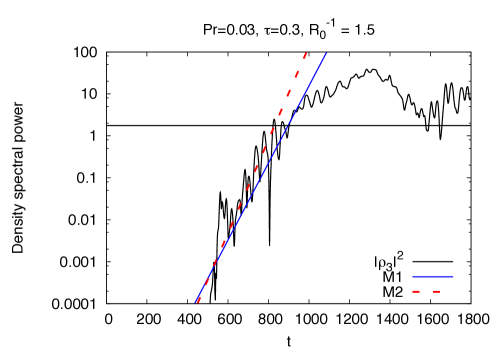
Applying the same method to all runs which eventually result in layer formation, we find that the layer growth rate predicted by the solution of equation (22) always correctly accounts for the observed mode growth in the simulations. Furthermore, while the growth rate predicted from experimentally-derived values of , , and is always better than the model-derived ones, the latter are nevertheless satisfactory estimates too, and are always within 10-30% of the correct value. These results complete the validation of Radko’s theory, as well as our model estimates for and .
7 Conclusion and prospects
The ultimate goal of this series of papers is to propose a new model for mixing by diffusive convection. In the work presented here, we ran and analyzed a very extensive suite of numerical simulations of the process in a wide range of parameter space. We have shown that in the astrophysically-relevant low Prandtl number (), low diffusivity ratio () regime, diffusive convection can take one of two forms depending on the local inverse density ratio : moderately efficient layered convection at lower , or inefficient wave-dominated “oscillatory” convection for higher (see Figure 1). We have confirmed through numerical and analytical work that a spontaneous transition into layered convection occurs, under predictable circumstances, through a linear mean-field instability of the initial state of oscillatory convection. This instability is called the instability. It was originally suggested in the oceanographic context of fingering convection by Radko (2003) and later applied to double-diffusive convection in astrophysics by Rosenblum et al. (2011).
Since transport in layered convection is much more efficient than in the non-layered case, a crucial element of any new model of diffusive convection will be the availability of a practical criterion for determining, for given , and , whether a system is expected to transition into layers or not, and on what timescale. The original instability theory provides such a criterion, but the latter can only be used in practice provided experimental measurements of the turbulent fluxes in homogeneous diffusive convection, for the same parameters, are available. We provide such measurements here for the planetary parameter regime, but similar results are unlikely to ever be available for the much more extreme stellar parameter regime.
Based on these considerations, we then proposed a new empirically motivated model for the turbulent fluxes, which enable us to derive a completely parameter-free semi-analytical criterion to determine, for any given fluid in the astrophysical regime () and any given stratification (), (a) whether a system is expected to transition into layers or not, and (b) on what timescales the layers are expected to emerge. Our model was found to fit the available numerical data very well, and can therefore be used very reliably within the same region of parameter space (e.g. the planetary parameter regime, for which ). We further propose that it should also be used in regions of parameter space for which fully resolved simulations are not available, namely in the stellar parameter regime (). Based on this model, we find that layered convection is theoretically expected in stellar interiors for a fairly wide range of parameter space, with between 1 and about 1000.
Our results answer, at least approximately, the first of the three questions we initially raised: (1) Under which conditions do layers form? (2) What is the transport rate in layered convection and (3) What is the transport rate in non-layered “oscillatory” convection. In subsequent papers in this series we will continue our investigation by answering questions (2) and (3).
Appendix A Appendix: Linear stability of semi-convection, asymptotic solutions for low Pr and , fastest-growing modes
The system of equations (9) can be linearized and solved for the fastest growing modes of diffusive convection. These linear solutions can then be studied further to obtain asymptotic scalings at very low Pr and , and to derive predictions for the turbulent buoyancy flux ratio (see Section 5).
A.1 Linearized equations for the fastest-growing modes
We first linearize (9)
around and ,
assuming all perturbations are normal modes of the form where . Hatted quantities
are now the amplitudes of the perturbations, while and are the horizontal wave-numbers, is the vertical
one, and is the growth rate. The latter are all
non-dimensional.
We are interested in the fastest-growing modes only, which can be shown to have as in the fingering case (Radko, 2003; Traxler et al., 2011b). They correspond to purely vertical fluid motions. They are rotationally invariant around the vertical direction, so without loss of generality we can align the horizontal wavenumber with the -axis choosing . After some simplifications, the resulting system of equations for the mode amplitudes are
| (A1) |
It has a non-trivial solution provided the growth rate satisfies the following cubic equation:
| (A2) |
In the regime of interest, this cubic has one negative real root and two complex conjugate roots (Baines & Gill, 1969). It can easily be shown that the complex conjugate roots ( with ) satisfy
| (A3) |
and that satisfies the cubic
| (A4) |
The latter has a positive solution if and only if where .
The fastest growing modes are determined by fixing Pr, and within the instability range, and finding the value of for which is maximum by solving (A4) in conjunction with , or in other words
| (A5) |
In what follows, we study the behavior of the solutions as a function of the reduced stratification parameter , defined in (26). Note that, with this new variable, we have
| (A6) |
A.2 Asymptotic solutions at low Pr and
In general, one needs to solve (A4) and (A5) numerically to find the fastest growing modes for given and . Here, however, we are interested in deriving asymptotic solutions for low Pr and low , since this is the parameter regime relevant for planetary and stellar interiors. In particular, we want to study how the growth rate and the wavenumber of the fastest-growing modes scale with these governing parameters.
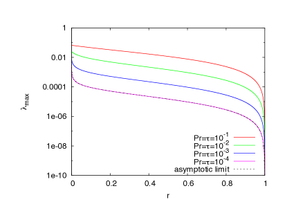
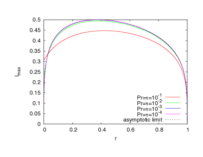
The solutions to equations (A4) and (A5) can easily be found numerically, and the results are shown in Figure 10 for decreasing Pr (here with Pr). We see that the real part of the fastest growing mode’s non-dimensional growth rate, , appears to be proportional to Pr, while the corresponding horizontal wavenumber, , becomes independent of Pr as Pr decreases.
This behavior suggests a new rescaling of the governing equations to capture the asymptotic regime () of the instability: where , and where . We also define , and assume that is order unity. Using (26) and keeping only the lowest terms in , equations (A4) and (A5) reduce to the simple universal444Note that this asymptotic limit is not uniformly valid for . system:
| (A7) |
This system still needs to be solved numerically for and , but only once for each value of and . Figure 10 compares the solution of (A7) with the ones obtained by direct numerical solution of (A4) and (A5) for and , and confirms our numerical and semi-analytical results.
This linear asymptotic analysis helps us estimate the growth rate of this kind of double-diffusive instability for a broad range of parameters and determine the size of the basic unstable structures we are interested in. Dimensionally speaking, our results imply that the true lengthscale of the instability should always be of the order of a few , where was defined in (8), and the growth rate of the instability should be of the order of where is the thermal buoyancy (Brünt-Väisälä) frequency. This information is useful for two reasons: first, to quantify the expected lengthscales or timescales in the real systems (i.e. stellar and planetary interiors), and secondly, to get some insight into the correct domain size and timestep to use in the numerical simulations.
A.3 Semi-analytical prediction for the turbulent buoyancy flux ratio
Let us consider the turbulent flux ratio
| (A8) |
where denotes a spatial average over the entire computational domain. Schmitt (1979) showed that it is possible to estimate this quantity for fingering convection using the velocity field, temperature and chemical composition perturbations corresponding to the linearly fastest-growing mode of instability. Since the unknown amplitude of the perturbations in this turbulent ratio cancels out, the remaining expression only depends on the known shape and growth rate of the perturbations. Here, we apply the same technique to estimate the turbulent flux ratio in diffusive convection.
From the system of equations (A1), we see that the amplitudes of the vertical velocity, temperature and compositional perturbations of a given mode are related via
| (A9) |
In order to calculate the fluxes, we must remember that, in the process of the linear analysis, the various fields , and were defined as complex variables, e.g. from , under the implicit understanding that only their real parts are physically meaningful. Hence, in practice,
| (A10) |
Without loss of generality, can be selected to be real so that
| (A11) |
Then, using (A9), we find that
| (A12) |
Finally, forming the turbulent flux ratio and integrating the relevant quantities over the computational domain and over short timescales (i.e. over at least one oscillation period of the basic instability), we get for a given mode with wavenumber and growth rate as
| (A13) |
where and are related via (A3). Applying this formula to the most rapidly growing mode, with wavenumber and growth rate calculated in Appendix A1, yields the required estimate for the inverse turbulent flux ratio in our simulations.
Appendix B Appendix B: Extraction of mean fluxes and results
B.1 Protocol for extracting mean fluxes and measuring from the simulations
In what follows, we describe our protocol for measuring the mean turbulent fluxes in the homogeneous phase of diffusive convection (prior to the emergence of large-scale structures). This involves first creating a systematic method to identify the start and end times of this phase and then estimating the fluxes and related errorbars.
B.1.1 Selection of .
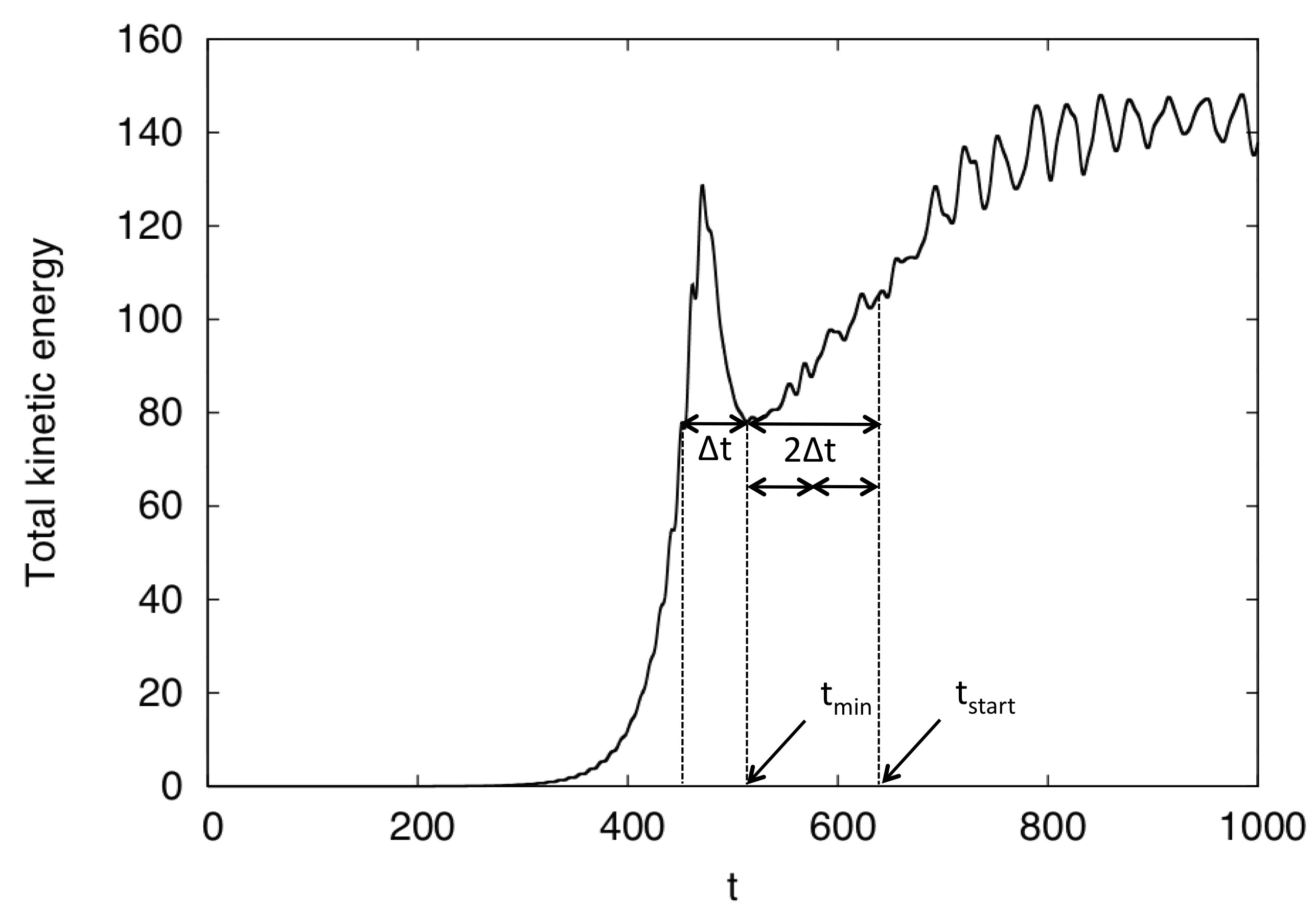
As seen in Figure 3, the turbulent flux typically peaks then drops quite sharply during the saturation of the primary instability, and then grows more slowly towards its value in the homogeneous double-diffusively convecting state. As shown in Figure 11, the same description applies to the behavior of the total kinetic energy in the system. It thus appears that the system needs a little bit of time to “recover” from the saturation. In order to extract meaningful averages, we therefore need to select the start of the averaging process well-past the main saturation peak. We also need to define in a manner that is meaningful across all simulations. Figure 11 illustrates our process: we define first the “width” of the saturation peak as illustrated, and then choose accordingly, about past the peak. While this choice is arguably somewhat arbitrary, it does satisfy the requirements listed above. Furthermore, the estimated values of are not particularly sensitive to the choice of as long as it is indeed well-past the saturation peak.
B.1.2 Selection of in the non-layered case
As noted earlier, by contrast with Rosenblum et al. (2011) we find that even in the non-layered case the system does not necessarily remain in a state of homogeneous, small-scale diffusive convection but sometimes becomes dominated by larger-scale coherent gravity waves555Rosenblum et al. (2011) did not notice the emergence of the waves in their simulations, although a more careful re-analysis of their results shows that they were indeed present in some of the higher runs.. While the precise reason for the emergence and synchronization of these waves remains to be determined, their associated dynamics lead to a rather different type of transport than in more homogeneous diffusive convection. For this reason, we must identify when the waves first “take over” and restrict our measurements of the turbulent fluxes prior to that time.
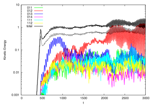
Shown in Figure 12 is the total kinetic energy in the simulation, as well as the total kinetic energy in the six highest-amplitude families of gravity wave modes. By “families”, we imply the following. A single gravity-wave mode, in this triply-periodic simulation, can be identified with the Fourier mode proportional to , where is the mode wave-vector. A “family” of modes is defined as the ensemble of all the modes with the same geometry given the symmetries of the system, i.e. the same values of and the same values of . In what follows, we classify the modes for simplicity of notation based on their periodicity: the single mode for example corresponds to one with , , . The family of modes 021 then corresponds to an ensemble of 8 modes: , , , , , , and finally . Finally, the total kinetic energy in the mode family is just the sum of that of the individual modes.
Figure 12 shows that the evolution of the total kinetic energy of the system is very similar to that of the turbulent fluxes for the same simulation (see Figure 3): an extended, apparently quasi-steady turbulent state between and , followed by a wave-dominated phase. It also reveals that the family of modes which dominates the system beyond is the 012 family, and that the strong oscillatory signal in the total kinetic energy (and the turbulent heat flux) appears when the total kinetic energy in that single family exceeds half the total kinetic energy of the system (shown as the thin black line).
We used a similar method to analyze every single simulation among the ones presented in Tables 1 and 2, comparing the total kinetic energy to that of various families of modes, and found that a robust (albeit empirical) criterion for determining the time when a system becomes dominated by gravity waves is simply that the total kinetic energy in any given family of modes exceeds half the total kinetic energy in the system. In the non-layered case, we therefore take the “end-point” of the temporal average to be . In some cases with close to marginal stability, it can happen that the start and end times thus selected have . When this is the case, we discard the simulation (for the purpose of estimating the turbulent fluxes and their ratio).
B.1.3 Selection of in the layered case
Applying the method described in the previous section we find that, in runs which eventually show the emergence of a staircase, gravity-wave modes never dominate the system. However, since we are interested here in the process which leads to layer formation, extracting the flux ratio in the layered case is only meaningful prior to the formation of the first layers. So, whenever layers appear in the simulations, we set to be the time where the first set of layers appears.
B.1.4 Averaging method and error estimates
Once the relevant time interval has been determined, we need to measure the mean turbulent fluxes, construct , and and estimate our experimental error. For this purpose, we use a “4-intervals” method: we first divide the integration domain previously defined into four sub-intervals, and calculate the mean fluxes and therefore , and in each one of them according to (23) and (24). The final adopted value of , and respectively is then the average of the four computed values, while the error is their standard deviation. The reason for using this method is clarified in the examples below.
Let us first illustrate our procedure on the data from the simulation shown in Figure 2a, i.e. for the run that leads to layer formation (with , ). We first estimate the start- and end-times of the homogeneous phase to be and . The mean , and in each sub-intervals are given in Table 4, as well as their final values and corresponding errorbars. These results illustrate the reason for using such a method to estimate the measurement “error” rather than a simple average over a single interval: the mean and increase steadily from one sub-interval to the other, showing that the system is not actually in a statistically quasi-steady state (as assumed by the instability theory). However, this clearly does not prevent the layering modes from growing anyway, and as shown in Section 6, the theory still adequately accounts for their growth rate despite the non-stationarity of the homogeneous phase. As such, we have to do the best with the data we have, and report on the values of , and accordingly, albeit with large errorbars which account for the slow temporal evolution of the system from saturation to the emergence of the staircase.
| Interval 1 | |||||
|---|---|---|---|---|---|
| Interval 2 | |||||
| Interval 3 | |||||
| Interval 4 | |||||
| Total |
Applying this method to the non-layered run shown in Figure 12 (with Pr=, ) we find that the start and end of the homogeneous period are and , and the corresponding , and computed are shown in Table 5. In this case the run is more stationary overall, leading to much smaller errorbars.
| Interval 1 | |||||
|---|---|---|---|---|---|
| Interval 2 | |||||
| Interval 3 | |||||
| Interval 4 | |||||
| Total |
B.2 Summary of the results
.
The results of our analysis are summarized in Tables 6 and 7.
| Pr | ||||||||
| Pr | ||||||||
References
- Baines & Gill (1969) Baines, P., & Gill, A. 1969, J. Fluid Mech., 37
- Chabrier & Baraffe (2007) Chabrier, G., & Baraffe, I. 2007, ApJ, 661, L81
- Guillot et al. (2004) Guillot, T., Stevenson, D. J., Hubbard, W. B., & Saumon, D. 2004, in Jupiter, ed. W. M. F. Bagenal, T.E. Dowling (Cambridge Univ. Press, Cambridge)
- Holton (1992) Holton, J. R. 1992, An introduction to dynamic meteorology, 3rd edition (San Diego, New York: Academic Press)
- Kato (1966) Kato, S. 1966, PASJ, 18, 374
- Linden & Shirtcliffe (1978) Linden, P. F., & Shirtcliffe, T. G. L. 1978, Journal of Fluid Mechanics, 87, 417
- Merryfield (1995) Merryfield, W. J. 1995, ApJ, 444, 318
- Radko (2003) Radko, T. 2003, J. Fluid Mech., 497, 365
- Rosenblum et al. (2011) Rosenblum, E., Garaud, P., Traxler, A., & Stellmach, S. 2011, ApJ, 731, 66
- Schmitt (1979) Schmitt, R. 1979, Deep-Sea Res., 26A, 23
- Schmitt et al. (2005) Schmitt, R., Ledwell, J., Montgomery, E., Polzin, K., & Toole, J. 2005, Science, 308, 685
- Schwarzschild & Härm (1958) Schwarzschild, M., & Härm, R. 1958, ApJ, 128, 348
- Spiegel & Veronis (1960) Spiegel, E. A., & Veronis, G. 1960, ApJ, 131, 442
- Spruit (1992) Spruit, H. C. 1992, A&A, 253, 131
- Stellmach et al. (2011) Stellmach, S., Traxler, A., Garaud, P., Brummell, N., & Radko, T. 2011, ArXiv e-prints
- Stern (1960) Stern, M. 1960, Tellus, 12, 172
- Stevenson (1982) Stevenson, D. J. 1982, Planet. Space Sci., 30, 755
- Timmermans et al. (2008) Timmermans, M.-L., Toole, J., Krishfield, R., & Winsor, P. 2008, Journal of Geophysical Research (Oceans), 113, C00A02
- Traxler et al. (2011b) Traxler, A., Garaud, P., & Stellmach, S. 2011b, ApJ, 728, L29
- Traxler et al. (2011a) Traxler, A., Stellmach, S., Garaud, P., Radko, T., & Brummell, N. 2011a, Journal of Fluid Mechanics, 677, 530
- Turner & Stommel (1964) Turner, J. S., & Stommel, H. 1964, Proceedings of the National Academy of Science, 52, 49
- Walin (1964) Walin, G. 1964, Tellus, 16, 389