Spin Dynamics of a $\mathbf{J}_{\mathbf{1}}$-$\mathbf{J}_{\mathbf{2}}$-$\mathbf{K}$ Model for the Paramagnetic Phase of Iron Pnictides

Abstract

We study the finite-temperature spin dynamics of the paramagnetic phase of iron pnictides within an antiferromagnetic $J_{1}-J_{2}$ Heisenberg model on a square lattice with a biquadratic coupling $-K(\mathbf{S}_{i}\cdot\mathbf{S}_{j})^{2}$ between the nearest-neighbor spins. Our focus is on the paramagnetic phase in the parameter regime of this $J_{1}-J_{2}-K$ model where the ground state is a $(\pi,0)$ collinear antiferromagnet. We treat the biquadratic interaction via a Hubbard-Stratonovich decomposition, and study the resulting effective quadratic-coupling model using both MSW and SBMF theories; the results for the spin dynamics derived from the two methods are very similar. We show that the spectral weight of dynamical structure factor $\mathcal{S}(\mathbf{q},\omega)$ is peaked at ellipses in the momentum space at low excitation energies. With increasing energy, the elliptic features expand towards the zone boundary, and gradually split into two parts, forming a pattern around $(\pi,\pi)$. Finally, the spectral weight is anisotropic, being larger along the major axis of the ellipse than along its minor axis. These characteristics of the dynamical structure factor are consistent with the recent measurements of the inelastic neutron scattering spectra on BaFe₂As₂ and SrFe₂As₂.

I Introduction

The emergence of superconductivity in iron pnictides Kamihara_FeAs ; Zhao_Sm1111_CPL08 near an antiferromagnetically ordered state Cruz in the phase diagram suggests strong interplay between the superconductivity and magnetism in these materials. Elucidating the magnetic excitations is therefore important for understanding not only the overall microscopic physics of these systems but also their superconductivity. In the parent compounds, the observed$(\pi,0)$ antiferromagnetic order arises either within a weak-coupling approach invoking a Fermi surface nesting,Graser ; Ran ; Knolle or from a strong-coupling approach whose starting point is a local moment $J_{1}-J_{2}-K$ model.Si ; Yildirim ; Ma ; Fang:08 ; Xu:08 ; Si_NJP ; Dai ; Uhrig

The strong-coupling approach is based on the proximity of the metallic ground state of the parent pnictides to a Mott localization transition, which gives rise to quasi-local magnetic moments.Si ; Si_NJP ; Haule ; Kutepov10 This incipient Mott picture corresponds to a ratio of $U$ (a measure of the Coulomb repulsions and Hund’s couplings among the Fe 3$d$ electrons) to $t$ (the characteristic bandwidth of the Fe 3$d$ electrons) which is not too far below the Mott threshold $U_{c}/t$, which is usually of order unity. This is supported by many experimental observations. For instance, the room-temperature electrical resistivity of parent iron pnictides is so large (even when the residual resistivity is relatively small signaling the smallness of elastic scattering) that the extracted mean-free path of quasiparticles would be comparable to the Fermi wavelength; this is typical of bad metals near a Mott trasition. Similarly, the Drude weight in optical conductivity Qazilbash ; Hu is strongly suppressed from its non-interacting counterpart, providing a direct measure of the proximity to the Mott transition. This is further corroborated by the the temperature-induced spectral weight transfer,Hu ; Yang ; Boris which is also characteristic of metals near a Mott transition. In the spin sector, zone boundary spin waves have been observed by inelastic neutron scattering (INS) measurements in the magnetically ordered state of several 122 iron pnictides compounds.Zhao Both the large spectral weight and the relatively-small spin damping suggest quasi-localized moments, which are expected near the Mott transition where the spin excitations arise out of incoherent electronic excitations. Additional evidence for the incipient Mott transition picture has come from the observation of a Mott insulating phase in the iron oxychalcogenides.Zhu This material contains an expanded Fe square lattice compared to the iron pnictides, which reduces $t$, thereby enhancing $U/t$ beyond $U_{c}/t$ (Ref. Zhu, ). Likewise, the Mott insulating behavior of the alkaline iron selenides MFang can also be interpreted as the result of a reduced effective $t$ and, correspondingly, an enhanced $U/t$ beyond $U_{c}/t$.Yu11 ; Zhou11

In the vicinity of $U_{c}/t$, where correlations are strong, it is natural that the spin Hamiltonian contains not only two-spin interactions, such as $J_{1}$ and $J_{2}$ Heisenberg exchange between nearest- and next-nearest- neighbor spins on a square lattice, but also interactions involving higher number of spins. These naturally include, for instance, the ring-exchange coupling involving four spins on a plaquette, and the biquadratic coupling of the form $-K(\mathbf{S}_{i}\cdot\mathbf{S}_{j})^{2}$ in systems with spin size $S\geqslant 1$.Fazekas The subject of the present study is to show how such non-Heisenberg interactions, particularly the biquadratic interaction, influence the spin dynamics in the paramagnetic phase.

Spin dynamics in the parent iron pnictides have been most extensively studied in the low-temperature state ($T<T_{N}$) with both antiferromagnetic order and orthorhombic structural distortion. Here, the INS experiments up to high energies (on the order of $200$ meV) show that the spin wave excitations in these compounds are highly anisotropic, with a dispersion which can be understood in terms of an anisotropic $J_{1x}-J_{1y}-J_{2}$ model with $J_{1x}\neq J_{1y}$.Zhao ; ZhaoSr ; Han09 . The anisotropy in the nearest-neighbor coupling is compatible with the orthorhombic structure, and its degree could reflect an orbital ordering.Singh ; Jaanen ; Lv ; AN Detailed theoretical studies of the magnetic excitations in the ordered phase have been carried out in such a $J_{1x}-J_{1y}-J_{2}$ model,Applegate and in a $J_{1}-J_{2}-K$ model.WysockiNP11 ; Stanek11 It should also be noted that terms such as the biquadratic coupling could be inferred from the sublattice angle dependence of the ground-state energy in LSDA calculations Yaresko , and were shown to appear naturally as a result of the orbital ordering between Fe d_xz and d_yz orbitals AN .

Our focus is instead on the spin dynamics in the paramagnetic phase of the parent iron pnictides, which has only recently been studied experimentally. The initial work by Diallo et al.Diallo measured the spin dynamics of CaFe₂As₂ at relatively low energies, below 70 meV. Theoretically, four of usGoswami11 studied the spin dynamics in the paramagnetic phase of the $J_{1}-J_{2}$ model (with or without an additional fermion damping). We showed that the experimentally observed elliptical features of the spin spectral weight in momentum space are well-described by this model and we determined the change to the elliptical features at high energies.

More recently, Harriger et al.Harriger reported measurements of the spin dynamics in the paramagnetic phase up to high energies (above 200 meV) in BaFe₂As₂. The INS measurements confirmed the quasi-two-dimensional spin dynamics found at low energies,Diallo and characterized the evolution of the low-energy elliptic features as they expand towards the zone boundary as the energy is raised, and determined the high-energy dispersion which appears to require a $J_{1x}\neq J_{1y}$ description even though the paramagnetic phase has a tetragonal structure. Similar data have also been reported by Ewings et al. in SrFe₂As₂.Ewings Theoretically, Park et al.ParkHauleKotliar11 analyzed the spin dynamics in the paramagnetic state within a dynamical mean-field theory (DMFT) for interactions $U/t\lessapprox U_{c}/t$, demonstrating that the DMFT approach captures key features of the neutron scattering results, including the ellipticity of the map of the structure-factor peak in the Brillouin zone.

In this paper, we study the spin dynamics of the $J_{1}-J_{2}-K$ model in the tetragonal paramagnetic phase using both modified spin wave (MSW) and Schwinger boson mean-field (SBMF) theories. The results from the two methods are in very good quantitative agreement with each other. We show that, for a moderate biquadratic coupling $K$, the dynamical structure factor $\mathcal{S}(\mathbf{q},\omega)$ has not only elliptic features near $(\pi,0)$, which expand with increasing energy and split into peaks surrounding $(\pi,\pi)$, but also an anisotropic distribution of the spectral weight that is larger along the major axis of each ellipse than along its minor axis. These properties agree well with the INS experiments Harriger ; Ewings

The remainder of the paper is organized as follows. In Sec. II we introduce the $J_{1}-J_{2}-K$ model and describe the MSW and SBMF theories used in this paper. In Sec. III we show how the biquadratic coupling $K$ influences the mean-field phase diagram and magnetic excitation spectrum. In Sec. IV we calculate the dynamical structure factor $\mathcal{S}(\mathbf{q},\omega)$. We also show that the spectral weight exhibits anisotropic features, discuss the evolution of the anisotropic features with increasing excitation energy, and explain how these properties arise from our theory. In Sec. V we first discuss some possible generalizations of the $J_{1}-J_{2}-K$ model we are studying in this paper. In the same section, we then consider the effect of itinerant electrons, and compare our study with other theoretical approaches to the spin dynamics. Sec. VI is devoted to a comparison with the INS experiments on the paramagnetic phases of the parent 122 iron pnictides, and Sec VII contains a few concluding remarks. In three appendices, we expound on the Ising transition at small $J_{1}/J_{2}$ ratios, and discuss the effects of both the ring-exchange interactions and interlayer exchange couplings.

II Model and Methods

The $J_{1}-J_{2}-K$ model is defined on a two-dimensional (2D) square lattice with the following Hamiltonian:

$$H = J_{1}\sum_{i,\boldsymbol{\delta}}\mathbf{S}_{i}\cdot\mathbf{S}_{i+\boldsymbol{\delta}}+J_{2}\sum_{i,\boldsymbol{\delta}^{\prime}}\mathbf{S}_{i}\cdot\mathbf{S}_{i+\boldsymbol{\delta}^{\prime}}$$ (1)

$$-K\sum_{i,\boldsymbol{\delta}}\left(\mathbf{S}_{i}\cdot\mathbf{S}_{i+\boldsymbol{\delta}}\right)^{2},$$

where $J_{1}$ and $J_{2}$ respectively denote the antiferromagnetic exchange couplings between spins located in the nearest neighbor ($\boldsymbol{\delta}=\hat{x}$,$\hat{y}$) and next-nearest neighbor ($\boldsymbol{\delta}^{\prime}=\hat{x}\pm\hat{y}$) sites. $K$ is the coupling for the biquadratic interaction between the nearest neighbor spin pairs.

To fully explain the experimentally observed $(\pi,0,\pi)$ antiferromagnetic order, an exchange coupling along the third dimension, $J_{z}$ should also be included. However, we find the model defined in Eq. (1) already allows us to understand the experimentally observed quasi-2D spin dynamics. Hence, we concentrate on this 2D model in the main text, and discuss the influence of the interlayer coupling $J_{z}$ on the spin dynamics in Appendix C.

The Hamiltonian of Eq. (1) is studied using both MSWTakahashi1 ; Takahashi2 and SBMFArovas methods. Here, we focus on the parameter regime where the ground state has a collinear $(\pi,0)$ antiferromagnetic order, and decompose the biquadratic interaction term of the Hamiltonian using two Hubbard-Stratonovich fields $\Gamma_{i,\hat{x}(\hat{y})}$. The effective Hamiltonian reads as

$$H = J_{1}\sum_{i,\boldsymbol{\delta}}\mathbf{S}_{i}\cdot\mathbf{S}_{i+\boldsymbol{\delta}}+J_{2}\sum_{i,\boldsymbol{\delta}^{\prime}}\mathbf{S}_{i}\cdot\mathbf{S}_{i+\boldsymbol{\delta}^{\prime}}$$ (2)

$$-2K\sum_{i,\boldsymbol{\delta}}\Gamma_{i,\boldsymbol{\delta}}\mathbf{S}_{i}\cdot\mathbf{S}_{i+\boldsymbol{\delta}}+K\sum_{i,\boldsymbol{\delta}}\Gamma_{i,\boldsymbol{\delta}}^{2}.$$

At the mean-field level, the Hubbard-Stratonovich fields are treated as static quantities, and can be expressed using equal-time spin correlators as: $\Gamma_{i,\boldsymbol{\delta}}=\langle\mathbf{S}_{i}\cdot\mathbf{S}_{i+\boldsymbol{\delta}}\rangle$. The Hubbard-Stratonovich transformation itself is exact. The static approximation is made in accordance with the level of approximation inherent to the MSW and SBMF methods, which incorporate static self-energies for the respective boson fields. As shown below, our approach has two important features: i) it is capable of studying the Ising correlations at nonzero temperatures; and ii) the MSW and SBMF approaches yield consistent results.

II.1 The modified spin wave theory

The MSW theory Takahashi1 ; Takahashi2 has been applied to the $J_{1}-J_{2}$ model by four of us.Goswami11 In this approach, a local spin quantization axis is defined at each site along the classical ordering direction $\mathbf{\Omega}_{i}^{cl}$. The Hamiltonian in Eq. (2) is then expressed in terms of Dyson-Maleev (DM) bosons via a local DM transformation: $\mathbf{S}_{i}\cdot\mathbf{\Omega}_{i}^{cl}=S-a^{\dagger}_{i}a_{i}$, $\mathbf{S}^{+}_{i}=\sqrt{2S}(1-a^{\dagger}_{i}a_{i}/2S)a_{i}$, and $\mathbf{S}^{-}_{i}=\sqrt{2S}a^{\dagger}_{i}$. Minimizing the free energy under the constraint of zero sublattice magnetization $\langle S-a^{\dagger}_{i}a_{i}\rangle=0$ by introducing a Lagrange multiplier $\mu$, and with respect to $\Gamma_{\delta}$ ($=\Gamma_{i,\boldsymbol{\delta}}$, by assuming translational symmetry), we obtain

$$\Gamma_{x} = \cos^{2}\frac{\phi}{2}f^{2}_{x}-\sin^{2}\frac{\phi}{2}g^{2}_{x},$$

$$\Gamma_{y} = \sin^{2}\frac{\phi}{2}f^{2}_{y}-\cos^{2}\frac{\phi}{2}g^{2}_{y},$$ (3)

where $\phi=\arccos(\mathbf{\Omega}_{i}^{cl}\cdot\mathbf{\Omega}_{i+\hat{x}}^{cl})$. $f_{\delta}=\langle a^{\dagger}_{i}a_{i+\boldsymbol{\delta}}\rangle$ and $g_{\delta}=\langle a_{i}a_{i+\boldsymbol{\delta}}\rangle$ are the ferromagnetic and antiferromagnetic bond operators, respectively. Minimizing the free energy with respect to $\phi$ gives either $\sin\phi=0$ for nonzero $f_{\delta}$ and $g_{\delta}$, or $\phi$ can be arbitrary if $f_{\delta}=g_{\delta}=0$. This defines two phases separated by a mean-field temperature scale Goswami11 $T_{\sigma 0}$: at $T>T_{\sigma 0}$, $\phi$ is arbitrary, and the system has $C_{4v}$ lattice rotational symmetry; while for $T<T_{\sigma 0}$, the $C_{4v}$ symmetry is broken and the system is Ising ordered, corresponding to either $\phi=0$ or $\phi=\pi$. In MSW theory, the Ising order parameter can be defined as $\sigma=2(\cos^{2}\frac{\phi}{2}(f^{2}_{x}+g^{2}_{y})-\sin^{2}\frac{\phi}{2}(f^{2}_{y}+g^{2}_{x}))$. From Eq. (II.1), if we define $\Gamma_{\pm}=(\Gamma_{x}\pm\Gamma_{y})/2$ as the symmetric and antisymmetric Hubbard-Stratonovich fields, we find that $\Gamma_{-}=\sigma/4$.

Minimizing the free energy with respect to other variational parameters, we obtain a set of self-consistent equations:

$$f_{\delta}=m_{0}+\frac{1}{\mathcal{N}}{\sum_{\mathbf{k}}}^{\prime}\frac{B_{\mathbf{k}}}{\varepsilon_{\mathbf{k}}}\left(n_{\mathbf{k}}+\frac{1}{2}\right)\cos(\mathbf{k}\cdot\boldsymbol{\delta}),$$ (4)

$$g_{\delta}=m_{0}+\frac{1}{\mathcal{N}}{\sum_{\mathbf{k}}}^{\prime}\frac{A_{\mathbf{k}}}{\varepsilon_{\mathbf{k}}}\left(n_{\mathbf{k}}+\frac{1}{2}\right)\cos(\mathbf{k}\cdot\boldsymbol{\delta}^{\prime}),$$ (5)

$$S+\frac{1}{2}=m_{0}+\frac{1}{\mathcal{N}}{\sum_{\mathbf{k}}}^{\prime}\frac{B_{\mathbf{k}}}{\varepsilon_{\mathbf{k}}}\left(n_{\mathbf{k}}+\frac{1}{2}\right),$$ (6)

where $\mathcal{N}$ is the total number of lattice sites, ${\boldsymbol{\delta}}=\hat{x},\hat{y}$, and ${\boldsymbol{\delta}^{\prime}}=\hat{x},\hat{y},\hat{x}\pm\hat{y}$. In Eqs. (4)-(6),

$$A_{\mathbf{k}} = 2\sin^{2}\frac{\phi}{2}\tilde{J}_{1x}g_{x}\cos k_{x}+2\cos^{2}\frac{\phi}{2}\tilde{J}_{1y}g_{y}\cos k_{y}$$ (7)

$$+4J_{2}g_{x+y}\cos k_{x}\cos k_{y},$$

$$B_{\mathbf{k}} = 4J_{2}g_{x+y}-\mu+2\sin^{2}\frac{\phi}{2}(\tilde{J}_{1x}g_{x}-\tilde{J}_{1y}f_{y}(1-\cos k_{y}))$$ (8)

$$+2\cos^{2}\frac{\phi}{2}(\tilde{J}_{1y}g_{y}-\tilde{J}_{1x}f_{x}(1-\cos k_{x})),$$

and the Bogoliubov angle $\theta_{\mathbf{k}}$ is defined via $\tanh 2\theta_{\mathbf{k}}=A_{\mathbf{k}}/B_{\mathbf{k}}$. The boson dispersion $\varepsilon_{\mathbf{k}}=\sqrt{B^{2}_{\mathbf{k}}-A^{2}_{\mathbf{k}}}$ and the boson number $n_{\mathbf{k}}=[\exp(\varepsilon_{\mathbf{k}}/k_{B}T)-1]^{-1}$. At $T=0$, the spectrum of the DM bosons becomes gapless at wave vector $\mathbf{Q}$ and $\mathbf{0}$. This corresponds to a long-range antiferromagnetic order at $\mathbf{Q}\neq 0$ with a nonzero spontaneous magnetization $m_{0}$. In this case, the summation ${\sum_{\mathbf{k}}}^{\prime}$ runs over all $\mathbf{k}$ values that make $\varepsilon_{\mathbf{k}}>0$, and the contribution from the $\varepsilon_{\mathbf{k}}=0$ terms is taken into account separately by $m_{0}$. For $T>0$, $m_{0}=0$, and the system is paramagnetic. Here the summation is performed in the full momentum space. In the presence of a small third-dimension coupling $J_{z}$, there will be a nonzero mean-field Néel temperature, $T_{N0}$; this is discussed in Appendix C.

Note that these self-consistent equations are exactly the same as those for the isotropic $J_{1}-J_{2}$ model.Goswami11 But the definitions of $A_{\mathbf{k}}$ and $B_{\mathbf{k}}$ are different. In Eqs. (7) and (8) above, we defined the effective exchange couplings $J_{1x}$ ($J_{1y}$) along the $x(y)$ direction as follows:

$$\tilde{J}_{1x(y)}=J_{1}-2K\Gamma_{x(y)},$$ (9)

expressed in terms of the Hubbard-Stratonovich fields $\Gamma_{x(y)}$ of spin-spin correlators in Eq. (II.1). Although in the $J_{1}-J_{2}-K$ model the bare nearest neighbor exchange coupling $J_{1}$ is still isotropic, a nonzero biquadratic coupling $K$ leads to an anisotropic effective coupling $\tilde{J}_{1x}\neq\tilde{J}_{1y}$ in the Ising ordered phase where $\Gamma_{x}\neq\Gamma_{y}$, i.e. the nearest-neighbor spin correlators along $x$ and $y$ are unequal, similarly to the situation found originallyChandra for the $J_{1}-J_{2}$ model.

II.2 The Schwinger boson theory

In the Schwinger boson representation,Arovas the SU($2$) spin operators are rewritten in terms of two Schwinger bosons via the transformation: $S_{i}^{z}=\frac{1}{2}(a_{i}^{\dagger}a_{i}-b_{i}^{\dagger}b_{i})$, $S_{i}^{+}=a_{i}^{\dagger}b_{i}$, and $S_{i}^{-}=b_{i}^{\dagger}a_{i}$. To limit the boson Hilbert space to the physical sector, a constraint $a_{i}^{\dagger}a_{i}+b_{i}^{\dagger}b_{i}=2S$ is imposed on each site. This can be generalized to the case of either SU($N$) ArovasAuerbach or SP($N$) ReadSachdev ; Flint spins, in either case there will be $N$ boson degrees of freedom at each site. For the experimentally observed $\mathbf{Q}=(\pi,0)$ or $(0,\pi)$ antiferromagnetic collinear phase in the 122 parent compounds, the $(ab)$-plane spin-spin correlations are expressed as:

$$\mathbf{S}_{i}\cdot\mathbf{S}_{j} = -(1-\Theta(i,j))[2\hat{g}_{ij}^{\dagger}\hat{g}_{ij}-S^{2}]$$ (10)

$$+\Theta(i,j)[2\hat{f}_{ij}^{\dagger}\hat{f}_{ij}-S(S+1)],$$

where $\hat{f}_{\delta}\!\equiv\!f_{i,i+\boldsymbol{\delta}}\!=\!\frac{1}{2}(a_{i}^{\dagger}a_{i+\boldsymbol{\delta}}+b_{i}^{\dagger}b_{i+\boldsymbol{\delta}})$ and $\hat{g}_{\delta}\!\equiv\!g_{i,i+\boldsymbol{\delta}}\!=\!\frac{1}{2}(a_{i}b_{i+\boldsymbol{\delta}}-b_{i}a_{i+\boldsymbol{\delta}})$ are respectively the ferromagnetic and antiferromagnetic bond operators. The function $\Theta(i,j)=1$ if $i$ and $j$ are on the same stripe sublattice, and $\Theta(i,j)=0$ if $i$ and $j$ are on different stripe sublattices. The Hubbard-Stratonovich field is then $\Gamma_{\delta}=|\hat{f}_{\delta}|^{2}-|\hat{g}_{\delta}|^{2}$, and in the case of $(\pi,0)$ ordering we find

$$\Gamma_{x} = -g^{2}_{x},$$

$$\Gamma_{y} = f^{2}_{y}.$$ (11)

Comparing this to Eq. (II.1), we see that the spin correlators coincide with those in the MSW theory if one sets $\phi=\pi$. Similarly, the case of $(0,\pi)$ ordering corresponds to $\phi=0$ in Eq. (II.1). In both cases, $\Gamma_{x}$ and $\Gamma_{y}$ have opposite sign, leading to the anisotropy in the effective spin-spin exchange couplings $\tilde{J}_{1x}\neq\tilde{J}_{1y}$, from Eq. (9).

By introducing Fourier transformation Ceccatto

$$a_{i} = \frac{1}{\sqrt{\mathcal{N}}}\sum_{\mathbf{k}}a_{\mathbf{k}}e^{i(\mathbf{k}-\frac{\mathbf{Q}}{2})\cdot\mathbf{r}_{i}},$$ (12)

$$b_{i} = \frac{1}{\sqrt{\mathcal{N}}}\sum_{\mathbf{k}}b_{\mathbf{k}}e^{i(\mathbf{k}+\frac{\mathbf{Q}}{2})\cdot\mathbf{r}_{i}},$$ (13)

and making a Bogoliubov transformation to a new quasiparticle creation/annihilation operators $\alpha_{k}=\cosh\theta_{\mathbf{k}}a_{\mathbf{k}}+i\sinh\theta_{k}b^{\dagger}_{-\mathbf{k}}$, one arrives at the mean-field free energy density, which can be generalized to the Sp($N$) form Flint

$$F_{MF} = \frac{NT}{\mathcal{N}}\sum_{\mathbf{k}}\ln\left[2\sinh\left(\frac{\omega_{\mathbf{k}}}{2T}\right)\right]+N\lambda\left(S+\frac{1}{2}\right)$$ (14)

$$- \frac{Nz}{8}\sum_{\boldsymbol{\delta}}J_{\boldsymbol{\delta}}(|f_{\boldsymbol{\delta}}|^{2}-|g_{\boldsymbol{\delta}}|^{2}),$$

where $z$ is the coordination number, and $\lambda$ is the Lagrange multiplier associated with the imposed constraint that on average, the number of bosons per site $\sum_{\sigma=1}^{N}n_{i\sigma}=NS$. Here $\omega_{\mathbf{k}}=\sqrt{(B_{\mathbf{k}}-\lambda)^{2}-A_{\mathbf{k}}^{2}}$ is the dispersion of the Bogoliubov quasiparticles, expressed Ceccatto in terms of the variables

$$A_{\mathbf{k}}=i\sum_{\boldsymbol{\delta}}J_{\boldsymbol{\delta}}\,g_{\boldsymbol{\delta}}\;e^{-i\mathbf{k}\cdot\boldsymbol{\delta}};\quad B_{\mathbf{k}}=\sum_{\boldsymbol{\delta}}J_{\boldsymbol{\delta}}\,f_{\boldsymbol{\delta}}\;e^{-i\mathbf{k}\cdot\boldsymbol{\delta}};$$ (15)

the Bogoliubov angle $\tanh 2\theta_{\mathbf{k}}\!=\!A_{\mathbf{k}}/(\lambda-B_{\mathbf{k}})$. The dispersion relation $\omega_{\mathbf{k}}$ explicitly depends on the ordering wave-vector ${\mathbf{Q}}$ and has minima around $\mathbf{k}=\pm\mathbf{Q}/2$. In the regime when $J_{2}>J_{1}/2$, the minimization of the free energy results in $\mathbf{Q}=(\pi,0)$ or $(0,\pi)$. For example, for $\mathbf{Q}=(\pi,0)$, the expressions for $A_{\mathbf{k}}$ and $B_{\mathbf{k}}$ become:

$$A_{\mathbf{k}} = 2\tilde{J}_{1x}g_{x}\sin k_{x}+4J_{2}g_{x+y}\sin k_{x}\cos k_{y},$$ (16)

$$B_{\mathbf{k}} = 2\tilde{J}_{1y}f_{y}\cos k_{y}.$$ (17)

In the large-$N$ limit of the Sp($N$) spin, the mean-field free energy Eq. (14) becomes exact.Arovas ; Flint The observable magnetic excitation spectrum is obtained from $\omega_{\mathbf{k}}$ by a $\mathbf{Q}/2$ shift: $\varepsilon_{\mathbf{k}}=\omega_{\mathbf{k}-\mathbf{Q}/2}$. At $T=0$, the magnetic order results in the gapless Goldstone modes at $\mathbf{k}=\mathbf{0}$ and $\mathbf{Q}$, as expected. The SBMF theory is known to reproduce well the spectrum of spin waves in both ferro- and antiferro-magnets.Arovas ; Ceccatto

Below, we focus on the paramagnetic phase at $T>0$, with short-range $\mathbf{Q}=(\pi,0)$ antiferromagnetic correlations (the case $\mathbf{Q}=(0,\pi)$ is obtained by $C_{4}$ lattice rotation). We obtain the following self-consistent equations from the saddle-point minimization of the free energy Eq. (14):

$$f_{\delta}=\frac{1}{\mathcal{N}}\sum_{\mathbf{k}}\frac{B_{\mathbf{k}}-\lambda}{\omega_{\mathbf{k}}}\left(n_{\mathbf{k}}+\frac{1}{2}\right)\cos\left(\mathbf{k}\cdot\boldsymbol{\delta}\right),$$ (18)

$$g_{\delta^{\prime}}=\frac{1}{\mathcal{N}}\sum_{\mathbf{k}}\frac{A_{\mathbf{k}}}{\omega_{\mathbf{k}}}\left(n_{\mathbf{k}}+\frac{1}{2}\right)\sin\left(\mathbf{k}\cdot\boldsymbol{\delta^{\prime}}\right),$$ (19)

$$S+\frac{1}{2}=\frac{1}{\mathcal{N}}\sum_{\mathbf{k}}\frac{B_{\mathbf{k}}-\lambda}{\omega_{\mathbf{k}}}(n_{\mathbf{k}}+\frac{1}{2}),$$ (20)

where $\boldsymbol{\delta}=\hat{y}$, and $\boldsymbol{\delta^{\prime}}=\hat{x},\hat{x}\pm\hat{y}$. Under the transformation $B_{\mathbf{k}}-\lambda\rightarrow B_{\mathbf{k}}$ and $\mathbf{k}\rightarrow\mathbf{k}-\mathbf{Q}/2$, Eqs. (16)-(20) in the SBMF theory and Eqs. (4)-(8) in the MSW mean-field theory have exactly the same form in the short-range $(\pi,0)$ correlated paramagnetic phase. Therefore, the two methods yield exactly the same mean-field phase diagram and boson dispersion, as corroborated by explicit numerical comparison. We further verified that these two theories give similar results for the spin dynamics of the $J_{1}-J_{2}-K$ model.

III Mean-field phase diagram and excitation spectrum

Figure 1: (Color online) Mean-field phase diagram in the MSW theory for $S=1$ and $J_{1}/J_{2}=1$. Phases I, II, and III respectively denote the $(\pi,0)/(0,\pi)$ long-range antiferromagnetically ordered state (at $T=0$), the Ising ordered paramagnetic state, and the isotropic paramagnetic state. The solid red curve refers to the mean-field temperature scale $T_{\sigma 0}=T_{0}$. In the shaded region the effective exchange coupling $\tilde{J}_{1y}<0$.

Figure 2: (Color online) The temperature evolution of the mean-field parameters in the MSW theory for $S=1$, $J_{1}/J_{2}=1$, and $K/J_{2}=0.8$.

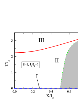
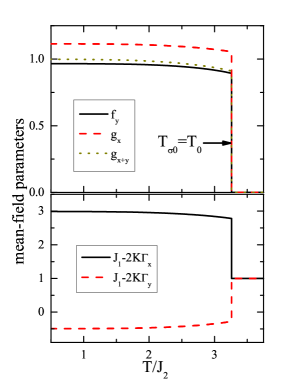
Since INS measurements suggest $J_{1}\sim J_{2}$ for several 122 compounds,Zhao ; Diallo ; Harriger our discussion on the $J_{1}-J_{2}-K$ model is focused on this parameter regime. Fig. 1 shows the mean-field phase diagram of the 2D $J_{1}-J_{2}-K$ model using the MSW method for $S=1$ and $J_{1}/J_{2}=1$. We identify three different phases. Phase I corresponds to the $(\pi,0)/(0,\pi)$ antiferromagneticaly long-range ordered phase; it exists only at $T=0$ in the 2D model. Phase II and phase III are both paramagnetic. They are separated by a mean-field Ising transition temperature $T_{\sigma 0}$. We find that for $J_{1}/J_{2}=1$, this transition is first-order, as shown in Fig. 2. But it can be either first-order or second-order for $J_{1}/J_{2}\lesssim 0.9$, as discussed in more detail in Appendix A. In the low-temperature phase II, either $f_{x}\neq f_{y}$ or $g_{x}\neq g_{y}$ (see Fig. 2), corresponding to an Ising ordered phase with either $(\pi,0)$ or $(0,\pi)$ short-range antiferromagnetic correlations. This Ising ordered phase already exists in the isotropic $J_{1}-J_{2}$ model.Chandra ; Flint ; Goswami11 But here, we find that a nonzero $K$ enhances $T_{\sigma 0}$, and $K$ drives the effective nearest-neighbor exchange couplings to be anisotropic. As shown in Fig. 2, in the $(\pi,0)$ Ising ordered phase (corresponds to $\phi=\pi$), the effective coupling $\tilde{J}_{1y}$ can even be ferromagnetic. This is important for understanding the experimentally observed anisotropic magnetic excitations at high energies in Ca-122Zhao and Ba-122.Harriger Phase III at $T>T_{\sigma 0}$ is the Ising disordered paramagnetic phase. In this phase the effective nearest-neighbor exchange couplings are isotropic because the nearest-neighbor bond correlators are zero. But the next-nearest-neighbor bond correlations may still be finite in this phase. One may define another temperature scale $T_{0}$, above which the next-nearest-neighbor bond correlations vanish and the system are decoupled into isolated local moments. Note that $T_{0}$ does not refer to a phase transition, and the discontinuity of the bond correlations at $T_{0}$ is an artifact of the mean-field theory.Takahashi1 In general, $T_{0}$ and $T_{\sigma 0}$ are two different temperature scales satisfying $T_{0}\geqslant T_{\sigma 0}$.Goswami11 ; Flint But for $J_{1}/J_{2}\gtrsim 0.9$, $T_{0}=T_{\sigma 0}$ for any $K/J_{2}$ ratio, as shown in Fig. 2. The phase diagram obtained in the SBMF theory is identical to the one shown in Fig. 1.

Figure 3: (Color online) (a): MSW dispersion along high symmetry directions in the paramagnetic Brillouin zone for the 2D $J_{1}-J_{2}-K$ model at $S=1$, $J_{1}/J_{2}=1.0$, $T/J_{2}=1.0$, and various $K$ values. For comparison, the red dashed curve shows the dispersion in the SBMF theory for the same parameters and $K/J_{2}=0.8$. The gaps at $(0,0)$ and $(\pi,0)$ are too small to be seen in the figure. (b): The symbols show the dispersion from the INS data at $T=150$ K in BaFe₂As₂, taken from Ref. Harriger, . The data can be fit by any of the theoretical dispersion curves [as in (a)] that lie within the shaded region.

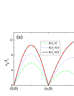
The finite coupling $K$ not only changes the phase boundary of the mean-field phase diagram, but can also dramatically influence the boson excitation spectrum. In Fig. 3(a), we show the dispersions of the DM and Schwinger bosons along two high-symmetry directions in momentum space for various $K$ values in phase II with $\phi=\pi$ using the same parameters as in Fig. 1. We see that the dispersion in Schwinger boson theory matches the one in the MSW theory exactly.

Figure 4: (Color online) Constant energy cuts of the rotational symmetrized spin dynamical structure factor in the momentum space in the MSW theory for $S=1$, $J_{1}/J_{2}=1.0$, $K/J_{2}=0.8$, and $T/J_{2}=1.0$. The corresponding energies are respectively $\omega=4J_{2}$ in (a), $\omega=10J_{2}$ in (b), $\omega=11.5J_{2}$ in (c), $\omega=12J_{2}$ in (d). In all the panels, a broadening factor $0.5J_{2}$ has been used for the convenience of calculation.

The dispersion shows a gap at $(\pi,0)$ (and also at $(0,0)$), with the size

$$\Delta_{1}=\sqrt{-\mu(8J_{2}g_{x+y}+4\tilde{J}_{1x}g_{x}-\mu)}.$$ (21)

At low temperatures the gap is small since $\mu\rightarrow 0$ as $T\ll T_{\sigma 0}$. In this limit, the excitation near $(\pi,0)$ can be approximated by $\varepsilon_{\mathbf{k}}=\sqrt{v_{1x}^{2}(\pi-k_{x})^{2}+v_{1y}^{2}k_{y}^{2}+\Delta_{1}^{2}}$, where the velocities are respectively:

$$v_{1x} = 4J_{2}g_{x+y}+2\tilde{J}_{1x}g_{x},$$ (22)

$$v_{1y} = \sqrt{(4J_{2}g_{x+y}+2\tilde{J}_{1x}g_{x})(4J_{2}g_{x+y}-2\tilde{J}_{1y}f_{y})+2\tilde{J}_{1y}f_{y}\mu}.$$

The excitation develops to the gapless Goldstone mode at $T=0$. At $(\pi,\pi)$ (and also at $(0,\pi)$) the dispersion has a different gap

$$\Delta_{2}=\sqrt{(8J_{2}g_{x+y}-4\tilde{J}_{1y}f_{y}-\mu)(4\tilde{J}_{1x}g_{x}-4\tilde{J}_{1y}f_{y}-\mu)}.$$ (24)

The features that $v_{1x}\neq v_{1y}$ and $\Delta_{1}\neq\Delta_{2}$ already exists in the isotropic $J_{1}-J_{2}$ model. In the $J_{1}-J_{2}-K$ model, $\Delta_{1}$ at $(\pi,0)$ is only weakly affected by $K$ because it is dominated by $\mu$. But $\Delta_{2}$ at $(\pi,\pi)$ is strongly influenced. It increases with $K$. For sufficiently large $K$, approximately where $\tilde{J}_{1y}$ changes sign to be ferromagnetic (the shaded region in Fig. 1), the dispersion at $(\pi,\pi)$ turns from a local minimum to a maximum, as shown in Fig. 3(a). Similar behavior in the spin-wave dispersion of the $J_{1}-J_{2}-K$ model has also been discussed in Ref. WysockiNP11, in the antiferromagnetically ordered phase, but our results apply to the paramagnetic phase.

IV Dynamical structure factor

In order to investigate the magnetic excitations, which are directly accessible by INS measurements, we have calculated the magnetic structure factor $\mathcal{S}({\mathbf{q},\omega})$. Our main interest is to understand the experimentally observed anisotropic feature of the magnetic excitations in the paramagnetic phase above the Néel temperature. As already discussed in Sec. III, in this temperature regime, the most relevant factor for the in-plane anisotropy is the Ising order. Therefore, we will concentrate our discussion on the magnetic structure factor in phase II of the 2D $J_{1}-J_{2}-K$ model. In this phase $\mathcal{S}({\mathbf{q},\omega})$ has the same form in both MSW and Schwinger boson theories,

$$\mathcal{S}({\mathbf{q},\omega)} = 2\pi\frac{C}{\mathcal{N}}{\sum_{\mathbf{k}}}^{\prime}\sum_{s,s^{\prime}=\pm 1}\left[\cosh(2\theta_{\mathbf{k}+\mathbf{q}}-2\theta_{\mathbf{k}})-ss^{\prime}\right]$$ (25)

$$\times\delta(\omega-s\varepsilon_{\mathbf{k}+\mathbf{q}}-s^{\prime}\varepsilon_{\mathbf{k}})n^{s}_{\mathbf{k}+\mathbf{q}}n^{s^{\prime}}_{\mathbf{k}},$$

where $\sum^{\prime}$ refers to the summation over the magnetic Brillouin zone corresponding to the $(\pi,0)$ order, which is enclosed by $-\pi/2\leqslant k_{x}\leqslant\pi/2$, and $-\pi\leqslant k_{y}\leqslant\pi$. $n^{+}_{\mathbf{k}}=n_{\mathbf{k}}+1$ and $n^{-}_{\mathbf{k}}=n_{\mathbf{k}}$. $C=1$ in the MSW theory, and $C=3/2$ in the Schwinger boson theory with SU($2$) symmetry.footnote We see from Eq. (25) that the contribution to $\mathcal{S}({\mathbf{q},\omega})$ comes from two-boson processes. Hence, in general cases the peak of $\mathcal{S}({\mathbf{q},\omega})$ does not follow the boson dispersion. But at low temperatures, the largest contribution to $\mathcal{S}({\mathbf{q},\omega})$ in the summation over $\mathbf{k}$ comes from the term at $\mathbf{k}=(0,0)$ since the small gap $\Delta_{1}$ at this point results in a large boson number $n_{\mathbf{k}}$. To satisfy the energy conservation in the $\delta$ function, $\mathcal{S}({\mathbf{q},\omega})$ must be peaked at $\omega\approx\varepsilon_{\mathbf{q}}$. Actually this leads to a two-peak structure corresponding to $s^{\prime}=\pm 1$ near $\omega=\varepsilon_{\mathbf{q}}$ for a fixed $\mathbf{q}$. But the separation of these two peaks is proportional to $\varepsilon_{(0,0)}$ and is very small at low temperatures. In the numerical calculations performed, the gap between the two peaks is healed by substituting the delta function by a Lorentzian with a small broadening width. As a result of this small broadening, $\mathcal{S}({\mathbf{q},\omega})$ only shows a single peak structure. Therefore, in this limit the peak positions of $\mathcal{S}({\mathbf{q},\omega})$ follow the boson dispersion.

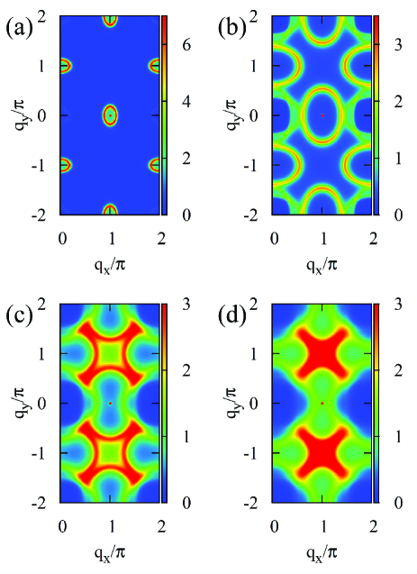
To better discuss the anisotropic distribution of the spectral weight in momentum space, we plot the constant energy cuts of the calculated $\mathcal{S}(\mathbf{q},\omega)$ at a fixed temperature $T<T_{\sigma 0}$ in Fig. 4. At low energies, the peaks of $\mathcal{S}(\mathbf{q},\omega)$ form a elliptic ring centered at $(\pi,0)$ (and also its symmetry related point $(0,\pi)$ after rotation symmetrization), as displayed in Figs. 4(a),(b). The elliptic feature is a consequence of the anisotropic correlation lengths in the Ising ordered phase, and the ellipticity near $(\pi,0)$ is proportional to $\xi_{x}/\xi_{y}=v_{1x}/v_{1y}$, which is not sensitive to temperature since the mean-field parameters are only weakly temperature dependent for $T<T_{\sigma 0}$ (Fig. 2). The ellipticity also only weakly depends on $K$: for $J_{1}/J_{2}=1$, we find $\xi_{x}/\xi_{y}\simeq 1.7$ at $K=0$, and $\xi_{x}/\xi_{y}\simeq 1.4$ at $K/J_{2}=0.8$.

With increasing energy, the ellipse centered around $(\pi,0)$ expands towards the Brillouin zone boundary, as seen in Figs. 4(a)-(d). For sufficiently large energy, the spectral weight reduces greatly along the $q_{x}$ direction, and the $\mathcal{S}(\mathbf{q},\omega)$ is peaked near $q_{y}=\pm\pi/2$ along the $q_{y}$ direction (Fig. 4(c)). The elliptical peak feature appears to have been split into two parts in the direction of its major axis. As the energy gets close to $\varepsilon_{(\pi,\pi)}$, the two peaks move towards $(\pi,\pm\pi)$, forming patterns that are centered around $(\pi,\pm\pi)$; cf. Figs. 4(c)-(d). In our theory, there are two factors that contribute to this anisotropic distribution of the spectral weight along the ellipses. Firstly, for $\omega>\varepsilon_{(\pi/2,0)}$, along the $q_{x}$ axis the energy conservation in the $\delta$ function of Eq. (25) can only be satisfied when $\mathbf{k}\neq(0,0)$. A nonzero $\mathbf{k}$ corresponds to a smaller $n_{\mathbf{k}}$, which greatly reduces $\mathcal{S}(q_{x},\omega)$. Along the $q_{y}$ axis, however, $\mathcal{S}(q_{y},\omega)$ is not reduced because the $\mathbf{k}=(0,0)$ mode can still satisfy the energy conservation. Secondly, for a given $\mathbf{k}$, the coherence factor $\cosh(2\theta_{\mathbf{k}}-2\theta_{\mathbf{k}+\mathbf{q}})$ along the ellipse is also anisotropic. To see this, recall that the largest contribution to $\mathcal{S}(\mathbf{q},\omega)$ is from the $\mathbf{k}=(0,0)$ term in Eq. (25). For simplicity, we take a single mode approximation, namely, $\mathcal{S}(\mathbf{q},\omega)$ can be approximated by this $\mathbf{k}=(0,0)$ term. Then the ellipse showing spectral weight peaks is determined by $\varepsilon_{\mathbf{q}}=\omega$, and the coherence factor $\cosh(2\theta_{\mathbf{k}}-2\theta_{\mathbf{k}+\mathbf{q}})\propto(B_{\mathbf{q}}-A_{\mathbf{q}})/\varepsilon_{\mathbf{q}}$. For $\sqrt{q_{x}^{2}\xi_{x}^{2}+q_{y}^{2}\xi_{y}^{2}}\ll T/\Delta_{1}$, $B_{\mathbf{q}}-A_{\mathbf{q}}\approx\Delta-\varepsilon_{\mathbf{q}}/\Delta-2\tilde{J}_{1y}f_{y}q_{y}^{2}$, where $\Delta=8J_{2}g_{x+y}+4\tilde{J}_{1x}g_{x}$. Since $\tilde{J}_{1y}<0$ for the choice of model parameters, it is easy to see that along the ellipse $\varepsilon_{\mathbf{q}}=\omega$, the maximum of the coherence factor is located along the $q_{y}$ axis but not the $q_{x}$ axis. Since within the single mode approximation, $\mathcal{S}(\mathbf{q},\omega)$ is proportional to the coherence factor, $\mathcal{S}(\mathbf{q},\omega)$ is also anisotropic along the ellipse. Note that at low energies ($\sqrt{q_{x}^{2}\xi_{x}^{2}+q_{y}^{2}\xi_{y}^{2}}\ll T/\Delta_{1}$), $\tilde{J}_{1y}f_{y}q_{y}^{2}\ll\Delta$, so the anisotropy is very small. This coherence-factor-induced anisotropy becomes sizable when the ellipse is large (for $\sqrt{q_{x}^{2}\xi_{x}^{2}+q_{y}^{2}\xi_{y}^{2}}\gtrsim T/\Delta_{1}$).

V Discussions

V.1 The effects of spin size

Figure 5: (Color online) (a): MSW dispersion along high symmetry directions in the paramagnetic Brillouin zone for the 2D $J_{1}-J_{2}-K$ model at $S=2$, $J_{1}/J_{2}=1.0$, $T/J_{2}=1.0$, and various $K$ values. (b): The ratio of $\tilde{J}_{1y}/\tilde{J}_{1x}$, showing the anisotropy in effective exchange couplings, see Eq. (9), as a function of the biquadratic coupling for $S=1$ and $S=2$.

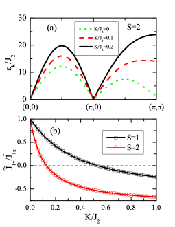
Besides the $S=1$ results shown in Sec. III and Sec. IV, we have also studied the $J_{1}-J_{2}-K$ model with larger spin sizes, and found the mean-field phase diagram is similar to the one in Fig. 1. Approximately, $T_{\sigma 0}$ and $T_{0}$ are increased by a factor of $S(S+1)/2$. The boson dispersion shown in Fig. 5(a) also exhibits the similar features as in the $S=1$ case. In Fig. 5(b) we compare the ratio of the effective nearest neighbor couplings $\tilde{J}_{1y}/\tilde{J}_{1x}$, defined in Eq. (9), for $S=1$ and $S=2$ (at zero temperature). We find that with increasing $S$, the minimal $K/J_{2}$ value where $\tilde{J}_{1y}$ becomes ferromagnetic is dropped from $K/J_{2}\approx 0.53$ to $K/J_{2}\approx 0.13$. Hence, we conclude that the anisotropy of the effective exchange couplings induced by non-Heisenberg coupling $K$ is more significant for larger spin size $S$.

We can further compare our MSW result at $T=0$ with the one in a recent MSW study, which used a mean-field treatment that is different from ours.Stanek11 The two theories yield exactly the same results when the spin size $S\to\infty$. For finite spin sizes, by comparing the behavior of $\tilde{J}_{1y}/\tilde{J}_{1x}$ ratio in Fig. 5(b) and the corresponding results in Ref. Stanek11, , we observe that the two theories give qualitatively similar results for the anisotropy in the exchange couplings: The biquadratic coupling $K$ reduces the ratio of the effective ratio $\tilde{J}_{1y}/\tilde{J}_{1x}$. Quantitatively, there are some differences between the two approaches. In particular, while for $S>1$, the ratio $\tilde{J}_{1y}/\tilde{J}_{1x}$ changes sign at a finite $K$ value in both theories, this sign change does not appear for $S=1$ in Ref. Stanek11, .

V.2 Generalizations of the $J_{1}-J_{2}-K$ model

Several remarks on the $J_{1}-J_{2}-K$ model studied in this paper. From the incipient Mott picture, when the system is in the vicinity of $U_{c}/t$, the spin Hamiltonian contains interactions involving more than just two spins. To see this, we start from a multi-orbital Hubbard model on a square lattice, and assume that Hund’s rule coupling locks the spins in different orbitals to a high spin state. Then we may obtain a spin-only Hamiltonian by integrating out the fermion degrees of freedom based on perturbation in $t/U$. To the $t^{2}/U$ order, we obtain the usual $J_{1}-J_{2}$ Heisenberg interaction between nearest- and next-nearest- neighbor spins. The next-order terms appear in the order $t^{4}/U^{3}$, and include the biquadratic $K$ term as well as the ring exchange interactions. Here, we have focused on the effects of the biquadratic interaction. The influence of the ring exchange interactions in the regime we are considering is briefly discussed in Appendix  B.

To fully understand the antiferromagnetic $(\pi,0,\pi)$ order revealed in the experiments, the 2D $J_{1}-J_{2}-K$ model needs to be extended to the 3D case by including an interlayer coupling $J_{z}$. A nonzero $J_{z}$ will support the antiferromagnetic order up to the Néel temperature $T_{N}$. In the mean-field treatment, the antiferromagnetic order emerges at a mean-field Néel temperature $T_{N0}$. The details of the effects of the interlayer coupling $J_{z}$ to the magnetic phase diagram of the $J_{1}-J_{2}-K$ model and the magnetic excitation spectrum is further discussed in Appendix  C.

When fluctuations beyond the mean-field level are taken into account, the actual Néel and Ising transition temperatures, $T_{N}$ and $T_{\sigma}$ can be well below their mean-field values. The mean-field temperatures $T_{N0}$ and $T_{\sigma 0}$ then correspond to some crossover temperature scales, below which the fluctuating order have significant effects. The fluctuating anisotropic effects we have presented will be dominant in the temperature regime $T_{N}<T<T_{\sigma 0}$.Goswami11

V.3 Effect of itinerant electrons

Within the bad-metal description of the iron pnictides, the quasi-localized moments are coupled to itinerant electrons with a spectral weight that depends on the proximity to the Mott transition. A convenient way to describe the effect of itinerant electrons on the spin dynamics is to reformulate the results of the local-moment-based calculations in terms of a non-linear sigma model, and introduce into the latter a damping caused by the itinerant electrons; for details, we refer to Ref. Goswami11, . Well below $T_{\sigma 0}$ and in the vicinity of $(\pi,0)$, the effects of the itinerant electrons are described in terms of the effective action for the staggered magnetization ${\bf M}$:

$$S[M] = T\int d{\bf q}\sum_{l}\left[r+\Delta r+v_{1x}^{2}q_{x}^{2}+v_{1y}^{2}q_{y}^{2}+\omega_{l}^{2}\right.$$ (26)

$$\left.+{\gamma}|\omega_{l}|\right]{\bf M}^{2}+u{\bf M}^{4}+\mathcal{O}({\bf M}^{6}).$$

Here, ${\bf M}=\mathbf{m}+\mathbf{m}^{{}^{\prime}}$ is the sum of ${\bf m}$ and ${\bf m^{\prime}}$, the O(3) vectors respectively for the magnetizations of the two decoupled sublattices on the square lattice, and $\omega_{l}$ the Matsubara frequency. This action arises in a “$w$-expansion”, which is based on a proximity to the Mott transition and is described in Refs. Si_NJP, ; Dai, ; it has the form of the usual $\sigma$-model nagaosa-book . In the first term, $\Delta r>0$ is a mass shift and $\gamma$ describes the strength of spin damping from coupling to fermions. (See Fig. 6) At relatively low energies, this introduces a procedure that can be used to describe the broadening of the spin spectral peaks in momentum space due to coupling to itinerant electrons.Goswami11

Figure 6: (Color online) Diagramm of the second-order contribution to the effective action in Eq. (26) due to coupling to fermions.

We should emphasize that this procedure is a qualitative treatment of the spin damping. Incorporating the full details of the electronic bandstructure will introduce momentum-dependence of the damping rate, making it possible to generate the type of anisotropic damping that was proposed phenomenologically by Harriger et al. Harriger .

Comparing our results for the $J_{1}-J_{2}-K$ model in Fig. 4(a)-(d) with those of the $J_{1}-J_{2}$ model (Fig. 4 of Ref. Goswami11, ) shows that, the biquadratic term itself brings out an anisotropy in the spectral weight of the elliptic peaks. The spectral weight is larger along the major axis of the ellipse than along its minor axis. This anisotropy goes in the same direction as that of the experimental data on BaFe₂As₂, illustrated in Fig. 4(f). We therefore conclude that both the ellipticity and intensity anisotropy of the spectral peaks in momentum space are controlled by the exchange interactions.

We note that the Ising order parameter is also coupled to the itinerant electrons. Since the Ising order parameter breaks the $C_{4v}$ symmetry, it couples to those spin singlet fermion bilinears that correspond to the $B_{1g}$ representation. Consequently a nonzero Ising order parameter will induce a nonzero $d_{x^{2}-y^{2}}$ nematic charge density $(\cos k_{x}-\cos k_{y})c_{\mathbf{k},\alpha}^{\dagger}c_{\mathbf{k},\alpha}$ for all the d-orbital electrons, where $\alpha$ is the orbital index. In addition the Ising order parameter will induce a nonzero charge density imbalance $c_{\mathbf{k}xz}^{\dagger}c_{\mathbf{k}xz}-c_{\mathbf{k}yz}^{\dagger}c_{\mathbf{k}yz}$ between the $d_{xz}$ and the $d_{yz}$ orbitals, which is also referred as the ferro-orbital order. As a result the spin fluctuations from the incoherent degrees of freedom can give rise to an orbitally ordered, charge nematic metal, with anisotropic transport properties. In a model with 3D coupling (see Appendix C), the coupling to the itinerant electrons will reduce the Néel transition temperature from its mean-field value $T_{N0}$ to $T_{N}<T_{N0}$, through the positive $\Delta r$ noted above. It will likewise decrease the Ising transition temperature from its mean-field value $T_{\sigma 0}$ to $T_{\sigma}<T_{\sigma 0}$. However, the correlation lengths are still sizeable and should be anisotropic up to $T_{\sigma 0}$.Goswami11 This implies that, in the 3D model with three-dimensional coupling, we expect anisotropic magnetic excitations to exist from $T_{N}$ all the way up to the crossover temperature scale $T_{\sigma 0}$, in the absence of a static Ising order.

V.4 Comparison with other approaches

Our studies in the $J_{1}-J_{2}-K$ model, with or without the coupling to the itinerant electrons, are very different from purely itinerant studies with $U/t$ much smaller than $U_{c}/t$. Because the Fermi surface comprises small electron and hole pockets, such calculations are expected to yield very small spin spectral weight. Experimentally, the total spectral weight is known to be large, with an effective moment that is larger than $1$ $\mu_{B}$/Fe in CaFe₂As₂ (Ref. Zhao, ). Such a large spectral weight arises naturally in our approach using as the starting point the $J_{1}-J_{2}$ model (with or without the $K$ term).

Our approach can be compared more closely with that of the DMFT studies of Ref. ParkHauleKotliar11, , in which the ratio of the effective interaction (combined Coulomb and Hund’s interactions) to the characteristic bandwidth is close to the Mott-transition value, $U/t\lessapprox U_{c}/t$. The proximity to the Mott transition ensures that a large part of the electronic spectral weight lies in the incoherent regime, which will naturally give rise to a large spin spectral weight. The consistency of the momentum-dependence determined by the DMFT calculations and that of our $J_{1}-J_{2}-K$ calculations further suggests the compatibility of the two approaches. There are some important differences, however. In the DMFT calculation, the anisotropy of the structure factor has been attributed to the geometry of the Fermi surface(s). The $J_{1}-J_{2}-K$ results however tie the anisotropy of the spin spectral weight in momentum space with the Ising correlations.

Experimentally, the Ising correlations can be very naturally connected with the $x-y$ anisotropy observed in ARPESYi and transportFisher measurements in the detwinned 122 iron pnictides at temperatures above $T_{N}$. A recent theoretical calculationFernandes shows how resistivity anisotropy in the tetragonal phase above $T_{N}$ follows from the existence of the Ising correlations discussed here.

Figure 7: (Color online) Evolution of $\mathcal{S}(\mathbf{q},\omega)$ in the paramagnetic phase of the $J_{1}-J_{2}-K$ model, showing that the elliptical features near $(\pi,0)$ at low energies (top panels) are split into features that are centered around $(\pi,\pi)$, as the energy is increased towards the zone-boundary spin-excitation energy (bottom panels). This trend is consistent with the inelastic neutron scattering experiments, shown in the box on the right for two energies measured in the paramagnetic phase of BaFe₂As₂ (data taken from Ref. Harriger, ). (a)-(d): Same as Fig. 4(a)-(d), but with damping $\gamma=3J_{2}$. (e)-(f): The INS data at $T=150$ K in BaFe₂As₂, taken from Ref. Harriger, . The energy transfer is $\omega=50\pm 10$ meV in (e), and $\omega=150\pm 10$ meV in (f). Here we find that the best agreement between theory and experimental data achieves when taking $J_{2}\approx 13$ meV in the model.

VI Comparison with experiments on the paramagnetic phases of parent 122 iron pnictides

Spin dynamics in the paramagnetic phase of the parent 122 iron pnictides has been recently studied via INS measurements.Diallo ; Harriger ; Ewings For CaFe₂As₂, spin dynamics at low energies (below $70$ meV) has been studied by Diallo et al.Diallo It is found that the peaks of the dynamical structure factor form anisotropic elliptic features at low energies, similar to the results in the antiferromagnetic phase.Zhao More recently, Harriger et al.Harriger measured the spin dynamics of BaFe₂As₂ up to $200$ meV. At low energies, they found the distribution of spectral weights in the momentum space forms similar elliptic feature as in the CaFe₂As₂ case. With increasing energy, the elliptic feature expands towards the Brillouin zone boundary. Moreover, they determined the magnetic dispersion to be peaked (or flat-topped) near $(\pi,\pi)$. Similar results have also been reported for SrFe₂As₂.Ewings

Our study on the $J_{1}-J_{2}-K$ model have already provided valuable information for understanding these experimental observations. In real materials, the various fluctuation mechanisms and the coupling to fermions/phonons will reduce the Néel and Ising transition temperatures. However, below the mean-field Ising temperature $T_{\sigma 0}$, the effective couplings between the nearest neighbors are always anisotropic. Hence we expect the magnetic fluctuations to be anisotropic for $T_{N}(\leq T_{\sigma})<T<T_{\sigma 0}$, which corresponds to the upper portion of region II in Fig. 1. This anisotropy is reflected in the spin dynamics in the paramagnetic phase.

To be specific, the anisotropic elliptic feature at low energies observed in CaFe₂As₂ and other parent 122 compounds can already been understood within the $J_{1}-J_{2}$ model.Goswami11 We have shown in Fig. 4 that the $J_{1}-J_{2}-K$ model gives the similar low-energy elliptic feature. It will be important to measure the spin dynamics at high energies in this material.

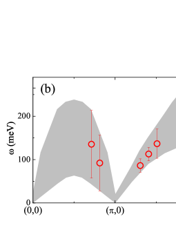
Our calculated evolution of this elliptic feature as the energy is raised in the $J_{1}-J_{2}-K$ model can be systematically compared with the experimental observations in BaFe₂As₂ and SrFe₂As₂. To see this, we fit the peak positions of calculated $\mathcal{S}({\mathbf{q},\omega})$ to the experimental magnetic excitation dispersion data in BaFe₂As₂, from which we can extract the best fitted values of the exchange couplings. Assuming $S=1$, we find the fitted exchange couplings are $J_{2}=17\pm 4$ meV, $J_{1}/J_{2}=1.0\pm 0.5$, and $K/J_{2}=0.8\pm 0.3$. We find that a very broad range of the $J_{1}/J_{2}$ ratio can all fit the experimental data quite well. As illustrated in Fig. 3(b), any dispersion curve within the shaded region fits the experimental data within error bars. But to fit the dispersion data near the local maximum at $(\pi,\pi)$, a moderate $K/J_{2}$ ratio is necessary. For $S=1$, we find $K/J_{2}\approx 0.8$ fits the data the best. On the other hand, for $S=2$, the best fitted $K/J_{2}$ ratio is substantially reduced to about $0.2$.

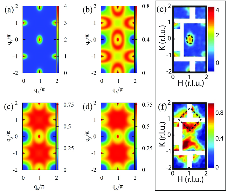
For BaFe₂As₂, detailed measurements in the momentum space have been reported by Harriger et al. Harriger . This allows us to see that the agreement between our theory and the experiment is not only for the dispersion, but also for the anisotropic distribution of the spectral weight of $\mathcal{S}(\mathbf{q},\omega)$ in momentum space.

In order to make a comparison with experimental data, we use Eq. (25) in the calculation of $\mathcal{S}(\mathbf{q},\omega)$ and approximate the delta function by the following Lorentzian broadening

$$\delta(\omega-\Delta\varepsilon)\longrightarrow\frac{1}{\pi}\frac{\gamma}{(\omega-\Delta\varepsilon)^{2}+\gamma^{2}}.$$ (27)

Here we have assumed that the broadening mainly comes from the damping effect due to coupling to itinerant electrons. It is then reasonable to take the phenomenological broadening factor to be the damping $\gamma$ introduced in Eq. (26) since in either the MSW or Schwinger boson theory, the damping is still due to the same bubble in Fig. 6. Calculating the magnitude of $\gamma$ requires a detailed microscopic theory and is beyond the scope of this article, however we can use Ref. Goswami11, for reference, where it has been determined that $\gamma/J_{2}\approx 3$ for CaFe₂As₂. Here we assume that this ratio still holds for BaFe₂As₂ and the damping is isotropic. In Figs. 7(a)-(d) we replot the theoretical dynamical spin structure factor in Fig. 4 with this damping factor, and compare them with the experimental data in Ref. Harriger, . At low energies, our theory correctly captures the elliptical feature centered at $(\pi,0)$ as displayed in Figs. 7(a),(b). Experimentally, this is seen as a filled elliptical spot due to damping effect, which is also shown in our theoretical plot in Fig. 7(a). The evolution of the elliptical feature with increasing energy is also consistent with the experimental observation: as the ellipse expands towards zone boundary, it gradually splits into two parts, and forms a pattern around $(\pi,\pi)$ (see Figs. 7(c), (d), and (f)). We reiterate that such anisotropic features are the properties of our $J_{1}-J_{2}-K$ model either with an isotropic or without additional damping due to itinerant electrons. While anisotropic damping proposed in Ref. Harriger, could reinforce the effect, it is not necessary to understand the INS experiments. In CaFe₂As₂ the elliptical feature around $(\pi,0)$ persists up to high energies, while in BaFe₂As₂, this elliptical feature splits into two parts at intermediate energy. Harriger These two different behaviors can both be understood within our $J_{1}-J_{2}-K$ model with similar, nearly isotropic damping but different $K$ values.

VII Conclusions

In this paper we have investigated the finite temperature spin dynamics of a $J_{1}-J_{2}-K$ antiferromagnetic Heisenberg model using both MSW and SBMF theories. The spin dynamics obtained from these two methods are similar to each other.

We have found that by including a moderate biquadratic coupling $K$, the magnetic excitation spectrum of the $J_{1}-J_{2}-K$ model is anisotropic below a mean-field Ising transition temperature $T_{\sigma 0}$. As in the case of the $J_{1}-J_{2}$ model Goswami11 , the peak of the low-temperature dynamical structure factor $\mathcal{S}(\mathbf{q},\omega)$ contains elliptical features near $(\pi,0)$ in the paramagnetic Brillouin zone at low excitation energies. However, unlike the pure $J_{1}-J_{2}$ model, the spectral intensity also displays anisotropy along the ellipse, with the intensity being higher along the major axis than that along the minor axis. This spectral anisotropy accounts for the observed particular way in which the low-energy elliptical features, centered around $(\pi,0)$, expand towards the zone boundary as the energy is increased towards the zone-boundary spin-excitation energy. It also gives rise to a particular form of high-energy spectral features that are centered around $(\pi,\pi)$.

We have also compared our calculated dynamical spin structure factor of the $J_{1}-J_{2}-K$ model with the recent inelastic neutron-scattering measurements in the paramagnetic phases of the 122 iron pnictides Harriger ; Diallo ; Ewings . The theoretical results provide a very natural understanding of the salient features of the experiments.

Appendix A Ising transition at small $J_{1}/J_{2}$ ratios

We find that the nature of the mean-field Ising transition at $T_{\sigma 0}$ depends on both $J_{1}/J_{2}$ and $K/J_{2}$ ratios. At $K=0$ and $J_{1}/J_{2}\lesssim 0.9$, we find $T_{\sigma 0}<T_{0}$, and the Ising transition at $T_{\sigma 0}$ is always second-order (Fig. 8). When $J_{1}/J_{2}\gtrsim 0.9$, $T_{\sigma 0}$ meets $T_{0}$ and the Ising transition becomes first-order. This is an artifact of the mean-field approximation since the transition at $T_{0}$ is always first-order.Takahashi1 ; Takahashi2 Still for $J_{1}/J_{2}\lesssim 0.9$, increasing $K$ from zero, the transition at $T_{\sigma 0}$ changes from second-order to first-order when $K$ is bigger than a bicritical point $K_{c}$. As shown in Fig. 8 for $J_{1}/J_{2}=0.6$, $K_{c}/J_{2}\approx 0.04$. At $K\gtrsim K_{c}$, $T_{\sigma 0}<T_{0}$. This suggests that the Ising transition near $K_{c}$ is not influenced by $T_{0}$ , but the order of this transition is tuned by $K$. Hence the first-order transition at $T_{\sigma 0}$ is not an artifact of the mean-field treatment.

Figure 8: (Color online) Mean-field magnetic phase diagram in the MSW theory for $S=1$, $J_{1}/J_{2}=0.6$. The dashed blue and dashed dotted brown curves refer to the mean-field temperature scales $T_{N0}$ and $T_{0}$, respectively. The thicker solid red curve refers to a second-order Ising transition at $T_{\sigma 0}$, while the thinner solid red curve refers to a first-order transition. In the shaded region, the effective exchange coupling $\tilde{J}_{1y}<0$.

Appendix B Effects of ring exchange couplings

Besides the quadratic and biquadratic interactions, other interactions involving more than two spins can also appear in the spin Hamiltonian in the vicinity of Mott transition. For instance, the four-spin ring exchange interaction can appear as a consequence of the fourth-order perturbation associated with the electron hopping process. We can consider the effects of a four-spin ring exchange process on the spin dynamics by adding a term $K_{\square}\sum_{i,j,k,l}[(\mathbf{S}_{i}\cdot\mathbf{S}_{j})(\mathbf{S}_{k}\cdot\mathbf{S}_{l})-(\mathbf{S}_{i}\cdot\mathbf{S}_{k})(\mathbf{S}_{j}\cdot\mathbf{S}_{l})+(\mathbf{S}_{i}\cdot\mathbf{S}_{l})(\mathbf{S}_{j}\cdot\mathbf{S}_{k})]$ to the Hamiltonian, where $K_{\square}>0$, and the sites $(i,j,k,l)$ are the vertices of a square plaquette, labeled clockwise. The four spin ring exchange competes against $J_{1}$ and $J_{2}$ and tends to weaken the antiferromagnetic order coming from $J_{1}$ or $J_{2}$. In the linear spin wave description of the $(\pi,0)$ ordered state, we obtain the effective exchange constants $\tilde{J}_{1x}=J_{1}+2(K-K_{\square})S^{2}$, $\tilde{J}_{1y}=J_{1}-2(K-K_{\square})S^{2}$, and $\tilde{J}_{2}=J_{2}+K_{\square}S^{2}$, and a reduced spin gap at $(\pi,\pi)$. This trend also persists in the paramagnetic state, and reduces the size of the Ising order parameter. For consistency with the experimental results we require $K>K_{\square}$.

Appendix C Effects of interlayer exchange coupling

Figure 9: (Color online) Mean-field magnetic phase diagram in the MSW theory for $S=1$, $J_{1}/J_{2}=1$, and an interlayer exchange coupling $J_{z}/J_{2}=0.1$. The dashed blue and solid red curves refer to the mean-field temperature scales $T_{N0}$ and $T_{\sigma 0}$, respectively. In the shaded region, the effective exchange coupling $\tilde{J}_{1y}<0$.

Figure 10: (Color online) The temperature evolution of the mean-field parameters in the MSW theory for $S=1$, $J_{1}/J_{2}=1$, $K/J_{2}=0.8$, and with an interlayer exchange coupling $J_{z}/J_{2}=0.1$.

Figure 11: (Color online) Dispersion of the $J_{1}-J_{2}-K$ model in the MSW theory for various $K$ values at $S=1$, $J_{1}/J_{2}=1.0$, $T/J_{2}=0.1$, and with an interlayer exchange coupling $J_{z}/J_{2}=0.1$.

The real materials have a 3D tetragonal structure. In the $J_{1}-J_{2}-K$ model, the 3D effects can be studied by extending the model to include a finite interlayer exchange interaction $J_{z}\sum_{i}\mathbf{S}_{i}\cdot\mathbf{S}_{i+\hat{z}}$. In 3D the long-range antiferromagnetic phase survives at finite temperature up to the Néel temperature $T_{N}$. In MSW and SBMF theories, the mean-field Néel temperature $T_{N0}$ is determined by the onset of spontaneous sublattice magnetization $m_{0}$. In general, $T_{N0}\leqslant T_{\sigma}\leqslant T_{0}$. The modification to our discussion in Sec. II comes through an additional interlayer antiferromanetic bond correlation parameter $g_{z}$. In the presence of $J_{z}$, the self-consistent equations of Eqs. (4)-(6) and Eqs. (18)-(20) are unchanged, but the expressions for $A_{\mathbf{k}}$ and $B_{\mathbf{k}}$ are modified according to

$$A_{\mathbf{k}}^{\mathrm{3D}} = A_{\mathbf{k}}+2J_{z}g_{z}\cos k_{z}$$ (28)

$$B_{\mathbf{k}}^{\mathrm{3D}} = B_{\mathbf{k}}+2J_{z}g_{z},$$ (29)

in the MSW mean-field theory, and

$$A_{\mathbf{k}}^{\mathrm{3D}} = A_{\mathbf{k}}+2J_{z}g_{z}\sin k_{z}$$ (30)

$$B_{\mathbf{k}}^{\mathrm{3D}} = B_{\mathbf{k}}.$$ (31)

in the SBMF theory.

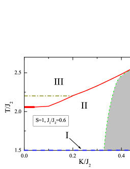
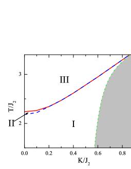
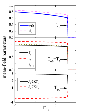
In Fig. 9 we show the phase diagram at the experimentally suggested ratio $J_{z}/J_{2}=0.1$. Similar to the 2D case, the mean-field phase diagram consists of an Ising and Néel ordered antiferromagnetic phase (I), an Ising ordered but Néel disordered paramagnetic phase (II), and an Ising and Néel disordered paramagnetic phase (III), separated by mean-field temperatures $T_{N0}$ and $T_{\sigma 0}$ (see also Fig. 10). For the parameters in Fig. 9, the transitions are both first-order, and both $T_{N0}$ and $T_{\sigma 0}$ increase with $K$. For $K/J_{2}\gtrsim 0.2$, $T_{N0}$ meets $T_{\sigma 0}$, and there is only a single transition between phases I and III. The absence of phase II in this regime is an artifact of the mean-field theory, since $T_{\sigma 0}$ is always bounded above by the mean-field scale $T_{0}$.

In connection to the real materials, we note that the structural and magnetic transitions in the 1111 pnictides are well separated. But in 122 compounds, they are either very close to each other, or become a single first-order transition. This can be understood in terms of the present theory, provided $J_{z}$ is stronger in the 122 materials. By comparing Fig. 9 and Fig. 2 we see that the magnetic transition is closer to the Ising transition for a larger $J_{z}$. Recent experiments also show that the electron doping may cause the separation of the structural and magnetic transition temperatures in Ba(Fe,Co)₂As₂ system.Rotundu11 The similarity between this behavior and the $K$ dependence of $T_{\sigma 0}$ and $T_{N0}$ in the phase diagram of Fig. 9 suggests the possibility that electron doping is positively correlated with a reduction of the biquadratic interaction. It would then be interesting to reveal the link between them in future experimental and theoretical studies.

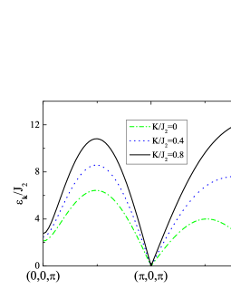
In Fig. 11 we show the low-temperature boson dispersions of the 3D model for various $K$ values along two high-symmetry directions in the $k_{z}=\pi$ plane. Aside from a larger gap at $(0,0,\pi)$, the dispersion is very similar to the one in 2D: the dispersion is highly anisotropic, and with increasing $K$, the local minimum at $(\pi,\pi,\pi)$ turns to a maximum. This is not too surprising because the in-plane anisotropy is a consequence of the 2D Ising-type fluctuations, and is not sensitive to the interlayer exchange coupling.

References

- (1) Y. Kamihara et al, J. Am. Chem. Soc. 130, 3296 (2008).
- (2) Z. A. Ren et al, Chin. Phys. Lett. 25, 2215 (2008).
- (3) C. de la Cruz et al., Nature 453, 899 (2008).
- (4) S. Graser et al, New J. Phys. 11, 025016 (2009).
- (5) Y. Ran et al, Phys. Rev. B 79, 014505 (2009).
- (6) J. Knolle et al, Phys. Rev. B 81, 140506(R) (2010).
- (7) Q. Si and E. Abrahams, Phys. Rev. Lett. 101, 076401 (2008).
- (8) T. Yildirim, Phys. Rev. Lett. 101, 057010 (2008).
- (9) F. Ma, Z-Y Lu, and T. Xiang, Phys. Rev. B 78, 224517 (2008).
- (10) C. Fang et al, Phys. Rev. B 77, 224509 (2008).
- (11) C. Xu, M. Muller, and S. Sachdev, Phys. Rev. B 78, 020501(R) (2008).
- (12) Q. Si, E. Abrahams, J. Dai, and J.-X. Zhu, New J. Phys. 11, 045001 (2009).
- (13) J. Dai et al. Proc. Natl. Acad. Sci. 106, 4118 (2009).
- (14) G. S. Uhrig et al., Phys. Rev. B 79, 092416 (2009).
- (15) K. Haule, J. H. Shim, and G. Kotliar Phys. Rev. Lett. 100, 226402 (2008).
- (16) A. Kutepov, K. Haule, S. Y. Savrasov, and G. Kotliar, Phys. Rev. B 82, 045105 (2010).
- (17) M. Qazilbash et al., Nat. Phys. 5, 647 (2009).
- (18) W. Z. Hu et al., Phys. Rev. Lett. 101, 257005 (2008).
- (19) J. Yang et al., Phys. Rev. Lett. 102, 187003 (2009).
- (20) A. V. Boris et al., Phys. Rev. Lett. 102, 027001 (2009).
- (21) J. Zhao et al., Nat. Phys. 5, 555 (2009).
- (22) J. X. Zhu et al., Phys. Rev. Lett. 104, 216405 (2010).
- (23) M. Fang et al., EuroPhys. Lett. 94, 27009 (2011).
- (24) R. Yu, J.-X. Zhu, and Q. Si, Phys. Rev. Lett. 106, 186401 (2011).
- (25) Y. Zhou, D.-H. Xu, F.-C. Zhang, and W.-Q. Chen, EuroPhys. Lett. 95, 17003 (2011).
- (26) P. Fazekas, Lecture Notes on Electron Correlation and Magnetism, World Scientific, Singapore, 1999, Chap. 5.
- (27) J. Zhao et al., Phys. Rev. Lett. 101, 167203 (2008).
- (28) M. J. Han, Q. Yin, W. E. Pickett, and S. Y. Savrasov, Phys. Rev. Lett. 102, 107003 (2009).
- (29) A. H. Nevidomskyy, preprint arXiv:1104.1747 (2011).
- (30) R. R. P. Singh, preprint arXiv:0903.4408 (2009).
- (31) F. Krüger et al., Phys. Rev. B 79, 054504 (2009).
- (32) W. Lv, F. Krüger and P. Phillips, Phys. Rev. B 82, 045125 (2010).
- (33) R. Applegate, J.Oitmaa, R. R. P. Singh, Phys. Rev. B 81, 024505 (2010)
- (34) A. L. Wysocki, K. D. Belashchenko, and V. P. Antropov, Nat. Phys. 7, 485 (2011).
- (35) D. Stanek, O. P. Sushkov, and G. S. Uhrig, Phys. Rev. B 84, 064505 (2011).
- (36) A. N. Yaresko, G.-Q. Liu, V. N. Antonov, and O. K. Andersen, Phys. Rev. B 79, 144421 (2009).
- (37) S. O. Diallo et al, Phys. Rev. B 81, 214407 (2010).
- (38) P. Goswami, R. Yu, Q. Si, and E. Abrahams, Phys. Rev. B 84, 155108 (2011).
- (39) L. W. Harriger et al., Phys. Rev. B 84, 054544 (2011).
- (40) R. A. Ewings et al., Phys. Rev. B. 83, 214519 (2011).
- (41) H. Park, K. Haule, and G. Kotliar, Phys. Rev. Lett. 107, 137007 (2011).
- (42) M. Takahashi, Phys. Rev. B 40, 2494 (1989).
- (43) M. Takahashi, Prog. of Theor. Phys. 101, 487 (1990).
- (44) A. Auerbach, and D. P. Arovas, Phys. Rev. Lett. 61, 617 (1988).
- (45) D. P. Arovas and A. Auerbach, Phys. Rev. B 38, 316 (1988).
- (46) N. Read and Subir Sachdev, Phys. Rev. Lett. 66, 1773 (1991).
- (47) R. Flint, and P. Coleman, Phys. Rev. B 79, 014424 (2009).
- (48) H. A. Ceccatto, C. J. Gazza, and A. E. Trumper, Phys. Rev. B bf 47, 12329 (1993).
- (49) P. Chandra, P. Coleman, and A. I. Larkin, Phys. Rev. Lett. 64, 88 (1990).
- (50) The factor in a or SBMF theory. Hence satisfies the sum rule only when . In the SBMF theory, violating the sum rule is a known issue. See Ref. Arovas, for more detail.
- (51) N. Nagaosa, Quantum Field Theory in Strongly Interacting Electronic Systems, Vol. II (Springer Verlag, Berlin 1999).
- (52) M. Yi et al., Proc. Natl. Acad. Sci. 108, 6878 (2011).
- (53) J. H. Chu et al., Science 329, 824 (2010).
- (54) R. M. Fernandes, E. Abrahams and J. Schmalian, Phys. Rev. Lett. 107, 217002 (2011).
- (55) C. R. Rotundu and R. J. Birgeneau, Phys. Rev. B 84, 092501 (2011).