Mysteries around the graph Laplacian eigenvalue 4
Abstract
We describe our current understanding on the phase transition phenomenon of the graph Laplacian eigenvectors constructed on a certain type of unweighted trees, which we previously observed through our numerical experiments. The eigenvalue distribution for such a tree is a smooth bell-shaped curve starting from the eigenvalue 0 up to 4. Then, at the eigenvalue 4, there is a sudden jump. Interestingly, the eigenvectors corresponding to the eigenvalues below 4 are semi-global oscillations (like Fourier modes) over the entire tree or one of the branches; on the other hand, those corresponding to the eigenvalues above 4 are much more localized and concentrated (like wavelets) around junctions/branching vertices. For a special class of trees called starlike trees, we obtain a complete understanding of such phase transition phenomenon. For a general graph, we prove the number of the eigenvalues larger than 4 is bounded from above by the number of vertices whose degrees is strictly higher than 2. Moreover, we also prove that if a graph contains a branching path, then the magnitudes of the components of any eigenvector corresponding to the eigenvalue greater than 4 decay exponentially from the branching vertex toward the leaf of that branch.
keywords:
graph Laplacian, localization of eigenvectors, phase transition phenomena, starlike trees, dendritic trees, Gerschgorin’s disksMSC:
15A22 , 15A42 , 65F15hide
1 Introduction
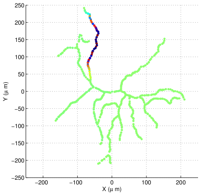
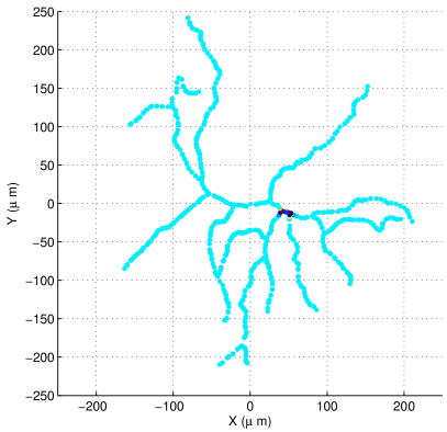
In our previous report [11], we proposed a method to characterize dendrites of neurons, more specifically retinal ganglion cells (RGCs) of a mouse, and cluster them into different cell types using their morphological features, which are derived from the eigenvalues of the graph Laplacians when such dendrites are represented as graphs (in fact literally as “trees”). For the details on the data acquisition and the conversion of dendrites to graphs, see [11] and the references therein. While analyzing the eigenvalues and eigenvectors of those graph Laplacians, we observed a very peculiar phase transition phenomenon as shown in Figure 1.1.
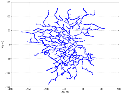
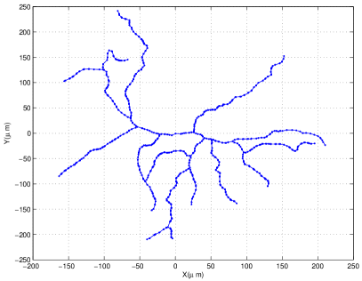
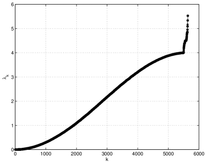
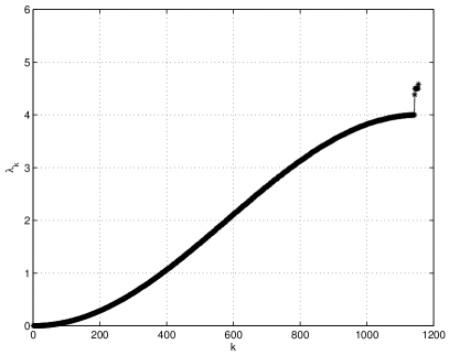
The eigenvalue distribution for each dendritic tree is a smooth bell-shaped curve starting from the eigenvalue 0 up to 4. Then, at the eigenvalue 4, there is a sudden jump as shown in Figure 1.1(c, d). Interestingly, the eigenvectors corresponding to the eigenvalues below 4 are semi-global oscillations (like Fourier cosines/sines) over the entire dendrites or one of the dendrite arbors (or branches); on the other hand, those corresponding to the eigenvalues above 4 are much more localized and concentrated (like wavelets) around junctions/branching vertices, as shown in Figure 1.2.
We want to answer the following questions:
- Q1
-
Why does such a phase transition phenomenon occur?
- Q2
-
What is the significance of the eigenvalue 4?
- Q3
-
Is there any tree that possesses an eigenvalue exactly equal to 4?
- Q4
-
What about more general graphs that possess eigenvalues exactly equal to 4?
As for Q1 and Q2, which are closely related, we have a complete answer for a specific and simple class of trees called starlike trees as described in Section 3, and a partial answer for more general trees and graphs such as those representing neuronal dendrites, which we discuss in Section 4. For Q3, we identify two classes of trees that have an eigenvalue exactly equal to 4, which is necessarily a simple eigenvalue, in Section 5.
In Section 6, we will prove that the existence of a long path between two subgraphs implies that the eigenvalues of either of the subgraphs that are larger than 4 are actually very close to some eigenvalues of the whole graph. Then, in Section 7, we will give a counterexample to the conjecture that the largest component in the eigenvector corresponding to the largest eigenvalue (which is larger than 4) lies on the vertex of the highest degree. Finally, we describe our investigation on Q4 in Section 8. But let us first start by fixing our notation and reviewing the basics of graph Laplacians in Section 2.
2 Definitions and Notation
Let be a graph where is a set of vertices in and is a set of edges where connects two vertices for some , and we write . Let be the degree of the vertex . If a graph is a tree, i.e., a connected graph without cycles, then it has edges. Let be the Laplacian matrix where is called the degree matrix of , i.e., the diagonal matrix of vertex degrees, and is the adjacency matrix of , i.e., if and are adjacent; otherwise it is 0. Furthermore, let be the eigenvalues of , and be the multiplicity of the eigenvalue . More generally, if is an interval of the real line, then we define .
At this point we would like to give a simple yet important example of a tree and its graph Laplacian: a path graph consisting of vertices shown in Figure 2.3.

The graph Laplacian of such a path graph can be easily obtained and is instructive.
The eigenvectors of this matrix are nothing but the DCT Type II basis vectors used for the JPEG image compression standard; see e.g., [14]. In fact, we have
| (2.1) | |||||
| (2.2) |
for , where is the eigenvector corresponding to . From these, it is clear that for any finite , , and no localization/concentration occurs in the eigenvector (or any eigenvector), which is simply a global oscillation with the highest possible (i.e., the Nyquist) frequency, i.e., .
3 Analysis of Starlike Trees
As one can imagine, analyzing this phase transition phenomenon for complicated dendritic trees turns out to be rather formidable. Hence, we start our analysis on a simpler class of trees called starlike trees. A starlike tree is a tree that has exactly one vertex of degree higher than 2. Examples are shown in Figure 3.4.


We use the following notation. Let be a starlike tree that has paths (i.e., branches) emanating from the central vertex . Let the th branch have vertices excluding . Let . Hence, the total number of vertices is .
Das proved the following results for a starlike tree in [3]:
| (3.3) |
On the other hand, Grone and Merris [7] proved the following lower bound for a general graph with at least one edge:
| (3.4) |
Hence we have the following
Corollary 3.1.
A starlike tree has exactly one graph Laplacian eigenvalue greater than or equal to 4. The equality holds if and only if the starlike tree is , which is also known as a claw.
Proof.
The first statement is easy to show. The lower bound in (3.4) is larger than or equal to 4 for any starlike tree since . On the other hand, the second largest eigenvalue is clearly strictly smaller than 4 due to (3.3).
To prove the second statement about the necessary condition on the equality (the sufficiency is easily verified), first note that by (3.4), is a necessary condition for . Then the Laplacian matrix of the starlike tree can be written as , where and are nonnegative integers ( are possibly empty). Let be the unit eigenvector of the claw (whose Laplacian is for the case ) corresponding to the eigenvalue . has the form where and . By the Courant-Fischer min-max characterization of eigenvalues [6, Theorem 8.1.2] we have
with the last equality holding if and only if , that is, when the starlike tree is the claw .
To prove the second statement about the necessary condition on the equality (the sufficiency is easily verified), first note that by (3.4), is a necessary condition for . Let denote the highest degree of such a starlike tree, i.e., . Since we only consider starlike trees, the second highest degree must be either 2 or 1. Now, we use the following
Theorem 3.1 (Das 2004, [4]).
Let be a connected graph and where and are the highest and the second highest degree, respectively. Then, if and only if is a star graph.
If and , then using this theorem, we must have . Hence, must be a star graph with and , i.e., . ∎
As for the concentration/localization of the eigenvector corresponding to the largest eigenvalue , we prove the following
Theorem 3.2.
Let , where is the value of the eigenvector corresponding to the largest eigenvalue at the vertex , . Then, the absolute value of this eigenvector at the central vertex cannot be exceeded by those at the other vertices, i.e.,
To prove this theorem, we use the following lemma, which is simply a corollary of Gerschgorin’s theorem [15, Theorem 1.1]:
Lemma 3.1.
Let be a square matrix of size , be any eigenvalue of , and be the corresponding eigenvector. Let denote the index of the largest eigenvector component in , i.e., where . Then, we must have , where is the th Gerschgorin disk of . In other words, for the index of the largest eigenvector component, the corresponding Gerschgorin disk must contain the eigenvalue.
Proof.
Recall the proof of Gerschgorin’s theorem. The th row of yields
This implies , which proves the lemma. ∎
Proof of Theorem 3.2.
First of all, by Corollary 3.1 we have . However, happens only for . In that case, it is easy to see that this theorem holds by directly examining the eigenvector . Hence, let us examine the case . In this case, Lemma 3.1 indicates where is the index of the largest component in . Now, note that the disk for any vertex that has degree 2 is (and for a degree 1 vertex). This means that the Gerschgorin disk containing the eigenvalue cannot be in the union of the Gerschgorin disks corresponding to the vertices whose degrees are 2 or lower. Hence the index of the largest eigenvector component in must correspond to an index for which the vertex has degree 3 or higher. In our starlike-tree case, there is only one such vertex, , i.e., . ∎
For different proofs without using Gerschgorin’s theorem, see Das [3, Lemma 4.2] and E. Woei’s dissertation [16]. We note that our proof using Gerschgorin’s disks is more powerful than those other proofs and can be used for more general situations than the starlike trees as we will see in Section 4.
Remark 3.1.
Let be an eigenvector of a starlike tree corresponding to the Laplacian eigenvalue . Without loss of generality, let be the vertices along a branch emanating from the central vertex with being the leaf (or pendant) vertex. Then, along this branch, the eigenvector components satisfy the following equations:
| (3.5) | |||||
| (3.6) |
From Eq. (3.6), we have the following recursion relation:
This recursion can be explicitly solved using the roots of the characteristic equation
| (3.7) |
and when (3.7) has distinct roots , the general solution can be written as
| (3.8) |
where are appropriate constants derived from the boundary condition (3.5). Now, let us consider these roots of (3.7) in detail. The discriminant of (3.7) is
Since we know that , this discriminant changes its sign depending on or . (Note that occurs only for the claw on which we explicitly know everything; hence we will not discuss this case further in this remark.) If , then and it is easy to show that the roots are complex valued with magnitude 1. This implies that (3.8) becomes
where satisfies , and are appropriate constants. In other words, if , the eigenvector along this branch is of oscillatory nature. On the other hand, if , then and it is easy to show that both and are real valued with while . On the surface, the term looks like a dominating part in (3.8); however, we see from (3.5) that , which means the real dominating part in (3.8) for is the term . Hence we conclude that decays exponentially with , that is, the eigenvector component decays rapidly towards the leaves. The siuation is the same for the other branches.
In summary, we have shown that a starlike tree has only one eigenvalue , and its eigenvector is localized at the central vertex in the sense of Theorem 3.1. Furthermore, the other eigenvectors are of oscillatory nature. Therefore the phase transition phenomenon for a starlike tree (with the eigenvalue 4 as its threshold) is completely understood.
4 The Localization Phenomena on General Graphs
Unfortunately, actual dendritic trees are not exactly starlike. However, our numerical computations and data analysis on totally 179 RGCs indicate that:
for each RGC. Hence, we can define the starlikeliness of a given tree as
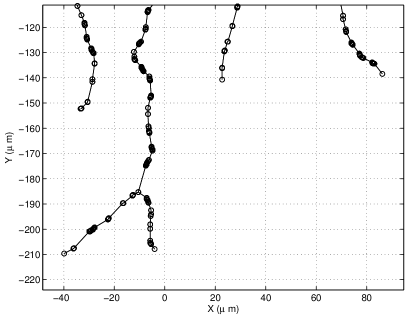
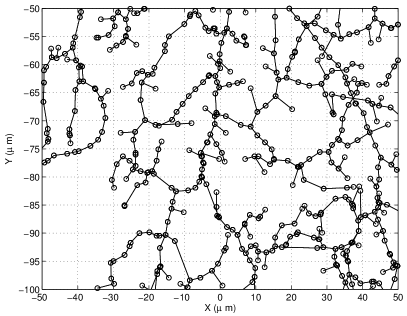
We note that for a certain class of RGCs whose dendrites are sparsely spread (see [11] for the characterization). This means that dendrites in that class are all close to a starlike tree or a concatenation of several starlike trees. We show some examples of dendritic trees with and with in Figure 4.5.
The above observation has led us to prove the following
Theorem 4.1.
For any graph of finite volume, i.e., , we have
and each eigenvector corresponding to has its largest component (in absolute value) on the vertex whose degree is higher than 2.
We refer the interested readers to [10, Sec. 2] that reviews various relationships between the multiplicity of certain eigenvalues and the graph structural properties different from our Theorem 4.1.
Proof.
The second statement follows from Lemma 3.1, because the Gerschgorin disks corresponding to vertices of degree 1 or 2 do not include .
We next prove the first statement. Let be a Laplacian matrix of . We can apply a permutation such that
| (4.9) |
where the diagonals of are 3 or larger (correspond to vertices of degree ), and the diagonals of are 2 or 1. Suppose is -by-. By Gerschgorin’s theorem all the eigenvalues of must be 4 or below.
In fact, we can prove the eigenvalues of are strictly below 4. By [15, Theorem 1.12], for an irreducible matrix (a Laplacian of a connected graph is irreducible) an eigenvalue can exist on the boundary of the union of the Gerschgorin disks only if it is the boundary of all the disks. Furthermore, if there is such an eigenvalue, then the corresponding eigenvector has the property that all its components have the same absolute value.
Suppose on the contrary that . Suppose without loss of generality that is irreducible; if not, we can apply a permutation so that is block diagonal and treat each block separately.
Now if has a diagonal 1, then the corresponding Gerschgorin disk lies on , which does not pass 4. Hence by [15, Theorem 1.12] this case is ruled out. It follows that all the diagonals of are 2, and the sum of the absolute values of the rows of are all 4 (this happens only if is disjoint from ). So we need (for example when , ). Now the th () row of and the fact force for all . This needs to hold for all , which clearly cannot happen for . Therefore the eigenvalues of must be strictly below 4.
By the min-max characterization of the eigenvalues of , denoting by the th smallest eigenvalue, we have
Hence letting be the last column vectors of the identity and noting , we have
Since , we conclude that (and hence ) has at least eigenvalues smaller than 4, i.e., . Hence, , which proves the first statement. ∎
To give a further explanation for the eigenvector localization behavior observed in Introduction, we next show that eigenvector components of must decay exponentially along a branching path.
Theorem 4.2.
Suppose that a graph has a branch that consists of a path of length , whose indices are where is connected to the rest of the graph and is the leaf of that branch. Then for any eigenvalue greater than 4, the corresponding eigenvector satisfies
| (4.10) |
where
| (4.11) |
Hence for , that is, the magnitude of the components of an eigenvector corresponding to any along such a branch decays exponentially toward its leaf with rate at least .
Proof.
There exists a permutation such that
where
and has a -1 in the top-right corner and 0 elsewhere. The diagonals of correspond to the vertices of the branch under consideration.
Let with . We have where . Note that . The last row of gives
hence
| (4.12) |
The st row of gives
Using we get
| (4.13) |
from which we get . Therefore , and so
Repeating this argument times we obtain (4.10). ∎
We note that the inequalities (4.12) and (4.13) include considerable overestimates, and tighter bounds can be obtained at the cost of simplicity. Hence in practice the decay rate is much smaller than defined in (4.11). We also note that the larger the eigenvalue , the smaller the decay rate is, i.e., the faster the amplitude decays along the branching path.
Also note that the above result holds for any branching path of a tree. In particular, if a tree has branches consisting of paths, they must all have the exponential decay in eigenvector components if . This gives a partial explanation for the eigenvector localization behavior observed in Introduction. However, the theorem cannot compare the eigenvector components corresponding to branches emanating from different vertices of degrees higher than 2, so a complete explanation remains an open problem.
Remark 4.1.
Let us briefly consider the case . In this case we have , suggesting the corresponding eigenvector components along a branching path may not decay. However, we can still prove that unless , we must have
| (4.14) |
In other words, the eigenvector components must decay along the branch, although not necessarily exponentially. To see this, we first note that if , then the last row of forces . Then, together with the st row gives . Repeating this argument we conclude that must be zero for all . Now suppose that . Following the above arguments we see that the inequality in (4.12) with must be strict, that is, . Using this we see that the inequality in (4.13) must also be strict, hence . Repeating this argument proves (4.14).
5 A Class of Trees Having the Eigenvalue 4
As raised in Introduction, we are interested in answering Q3: Is there any tree that possesses an eigenvalue exactly equal to 4? To answer this question, we use the following result of Guo [9] (written in our own notation).
Theorem 5.1 (Guo 2006, [9]).
Let be a tree with vertices. Then,
and the equality holds if and only if all of the following hold: a) ; b) divides ; and c) is spanned by vertex disjoint copies of .
Here, a tree is said to be spanned by vertex disjoint copies of identical graphs for if and for all . Figure 5.6(a) shows an example of such vertex disjoint copies for by connecting their central vertices. We note that there are many other ways to form disjoint vertex copies of .
This theorem implies the following
Corollary 5.1.
A tree has an eigenvalue exactly equal to 4 if it is spanned by vertex disjoint copies of .

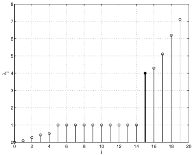
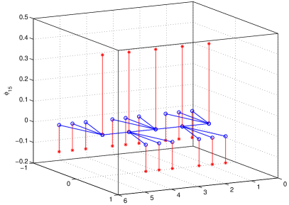
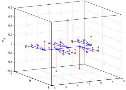
Figure 5.6(b) shows the eigenvalue distribution of a tree spanned by copies of as shown in Figure 5.6(a). Regardless of , the eigenvector corresponding to the eigenvalue 4 has only two values: one constant value at the central vertices, and the other constant value of the opposite sign at the leaves, as shown in Figure 5.7(a). By contrast, the eigenvector corresponding to the largest eigenvalue is again concentrated around the central vertex as shown in Figure 5.7(b).
Theorem 5.1 asserts that a general tree with vertices can have at most Laplacian eigenvalues . We also know by Theorem 2.1 of [8] that any tree possessing the eigenvalue must have multiplicity and for some . Hence, Theorem 5.1 also asserts that trees spanned by vertex disjoint copies of form the only class of trees for which 4 is the th eigenvalue of ; in other words, trees in this class are the only ones that have exactly eigenvalues .
Trees spanned by vertex disjoint copies of , however, are not the only ones that have an eigenvalue exactly equal to 4. For instance, Example 2.9 of [8], which has vertices and is called as shown in Figure 5.8, is non-isomorphic to any tree spanned by 9 vertex disjoint copies of ; yet it has (but ).
On the other hand, we have the following
Proposition 5.1.
If , any tree possessing an eigenvalue exactly equal to 4 must be spanned by vertex disjoint copies of .
Proof.
First of all, 4 must divide , hence with or . If , then we know from Theorem 5.1 that and . Hence, is the only possibility, and consequently using the same theorem. If , then Theorem 5.1 states that ; ; and ; …If , then the necessary and sufficient conditions for the equality in Theorem 5.1 state that must be spanned by two vertex disjoint copies of , so we are done. Now we still need to show that cannot be 4. Let be the degree of the highest degree vertex of a tree under consideration. Then, we have
| (5.15) |
Here, the lower bound is due to Grone and Merris [7] and the upper bound is due to Stevanović [13]. Now, we need to check a few cases of the values of .
-
1.
If , then the upper bound in (5.15) is 4. Hence, cannot happen. (This includes the case of a path graph that cannot reach the eigenvalue 4). So, we must have .
-
2.
If , of course, the lower bound in (5.15) is greater than 4. Hence, cannot be 4 either.
-
3.
Finally, if , then the above bounds are: . Can in this case? According to Zhang and Luo [17], the equality in that lower bound holds if and only if there exists a vertex that is adjacent to all the other vertices in . That is, the degree of that vertex is . Since , this cannot happen.
Hence, for , the only possibility for a tree to have an eigenvalue exactly equal to 4 is the case when , which happens if and only if is spanned by two vertex disjoint copies of . ∎
It turns out, however, that proving the necessity for using similar arguments quickly becomes cumbersome, even for the next step . At this point, we do not know whether there are other classes of trees than discussed above or those spanned by vertex disjoint copies of that can have an eigenvalue exactly equal to 4. Hence, identifying every possible tree that has an eigenvalue exactly equal to 4 is an open problem.

6 Implication of a Long Path on Eigenvalues
In Section 4 we saw that for a graph that has a branch consisting of a long path, its Laplacian eigenvalue greater than 4 has the property that the corresponding eigenvector components along the branch must decay exponentially.
Here we discuss a consequence of such a structure in terms of the eigenvalues. We consider a graph formed by connecting two graphs and with a path . Note that this is a more general graph than in Section 4 (which can be regarded as the case without ). We show that if is a long path then any eigenvalue greater than 4 of the Laplacian of either of the two subgraphs and must be nearly the same as an eigenvalue of the Laplacian of the whole graph .
Theorem 6.1.
Let be a graph obtained by connecting two graphs with a path, whose Laplacian can be expressed as
where and have -1 in the top-right corner and 0 elsewhere. is for and represents the path , that is, a tridiagonal matrix with 2 on the diagonals and -1 on the off-diagonals.
Let be any eigenvalue of the top-left (or bottom-right ) submatrix of . Then there exists an eigenvalue of such that
| (6.16) |
where .
Proof.
We treat the case where is an eigenvalue of the top-left part of , which we denote by . The other case is analogous.
As in Theorem 4.2, we can show that any eigenvalue of has its corresponding eigenvector components decay exponentially along the path . This means that the bottom eigenvector component is smaller than in absolute value (we normalize the eigenvector so that it has unit norm) where as in (4.11).
Let be an eigendecomposition where and the eigenvalues are arranged so that appears in the top diagonal of . For notational convenience let . Then, consider the matrix
| (6.17) |
where and . Direct calculations show that where is the bottom component of the eigenvector of corresponding to the th eigenvalue. In particular, by the above argument we have .
Note that in the first row and column of , the only nonzeros are the diagonal (which is ), and the and entries, both of which are equal to . Now, viewing the and entries of as perturbations (write where is obtained by setting the and entries of to 0) and using Weyl’s theorem [6, Theorem 8.1.5] we see that there exists an eigenvalue of (and hence of ) that lies in the interval . Together with we obtain (6.16). ∎
Recall that decays exponentially with , and it can be negligibly small for moderate ; for example, for we have . We conclude that the existence of a subgraph consisting of a long path implies that the eigenvalues of a subgraph must match those of the whole graph to high accuracy.
7 On the Eigenvector of the Largest Eigenvalue
In view of the results in Section 4 it is natural to ask whether it is always true that the largest component of the eigenvector corresponding to the largest eigenvalue of a Laplacian matrix of a graph lies on the vertex of the highest degree. Here we show by a counterexample that this is not necessarily true.
Consider for example a tree as in Figure 7.9, which is generated as follows: first we connect copies of (equal to ) as shown in Figure 5.6(a); then add to the right a comet as in Figure 3.4(b).

Now for sufficiently large and ( is sufficient), the largest component in the eigenvector corresponding to the largest eigenvalue of the resulting Laplacian occurs at one of the central vertices of , not at the vertex of degree 5 belonging to the comet.
Let us explain how we came up with this counterexample. The idea is based on two facts. The first is the discussion in Section 6, where we noted that a long path implies any eigenvalue larger than 4 must be close to an eigenvalue of a subgraph or . Therefore, in the notation of Section 6, by connecting two graphs ( and , a star) with a path such that the largest eigenvalue of is larger than that of , we ensure that the largest eigenvalue of is very close to . The second is the Davis-Kahan theorem [5], which states that a small perturbation of size in the matrix (recall the proof of Theorem 6.1) can only induce small perturbation also in the eigenvector: its angular perturbation is bounded by , where is the distance between and the eigenvalues of after removing its first row and column. Furthermore, the eigenpair of satisfies , and the eigenvectors ( by Davis-Kahan) of and of corresponding to are related by , which follows from (6.17). Therefore, has its large components at the vertices belonging to . In view of these our approach was to find two graphs and such that the highest degrees of the vertices of and are 4 and 5, respectively, and the largest eigenvalue of the Laplacian of is larger than that of .
8 Discussion
In this paper, we obtained precise understanding of the phase transition phenomenon of the combinatorial graph Laplacian eigenvalues and eigenvectors for starlike trees. For a more complicated class of graphs including those representing dendritic trees of RGCs, we proved in Theorem 4.1 that the number of the eigenvalues greater than or equal to 4 is bounded from above by the number of vertices whose degrees are strictly higher than 2. In Theorem 4.2, we proved that if a graph has a branching path, the magnitude of the components of an eigenvector corresponding to any eigenvalue greater than 4 along such a branching path decays exponentially toward its leaf. In Remark 4.1, we also extended Theorem 4.2 for the case of although the decay may not be exponential.
As for Q3 raised in Introduction—“Is there any tree that possesses an eigenvalue exactly equal to 4?”—we showed that any tree with vertices ( for some ) spanned by vertex disjoint copies of possesses an eigenvalue exactly equal to 4 in Corollary 5.1, and that such class of trees are the only ones that can have an eigenvalue exactly equal to 4 if in Proposition 5.1. On the other hand, for larger , we pointed out that not only those spanned by vertex disjoint copies of , but also a tree called discovered in [8] and shown in Figure 5.8 have an eigenvalue exactly equal to 4. A challenging yet interesting question is whether or not one can identify every possible tree that has an eigenvalue 4.
Another quite interesting question is Q4 raised in Introduction: “Can a simple and connected graph, not necessarily a tree, have eigenvalues equal to 4?” The answer is a clear “Yes.” For example, the -cube (), i.e., the -fold Cartesian product of with itself is known to have the Laplacian eigenvalue 4 with multiplicity ; see e.g., [1, Sec. 4.3.1].
Another interesting example is a regular finite lattice graph in , , which is simply the -fold Cartesian product of a path shown in Figure 2.3 with itself. Such a lattice graph has repeated eigenvalue 4. In fact, each eigenvalue and the corresponding eigenvector of such a lattice graph can be written as
| (8.18) | |||||
| (8.19) |
where for each , as shown by Burden and Hedstrom [2]. Note that (8.18) and (8.19) are also valid for . In that case these reduce to (2.2) that we already examined in Section 2.
Now, determining , i.e., the multiplicity of the eigenvalue 4 of this lattice graph, is equivalent to finding the number of the integer solutions to the following equation:
| (8.20) |
For , there is no solution as we mentioned in Section 2. For , it is easy to show that by direct examination of (8.20) using some trigonometric identities. For , behaves in a much more complicated manner, which is deeply related to number theory. We expect that more complicated situations occur for . We are currently investigating this on regular finite lattices. On the other hand, it is clear from (8.19) that the eigenvectors corresponding to the eigenvalues greater than or equal to 4 on such lattice graphs cannot be localized or concentrated on those vertices whose degree is higher than 2 unlike the tree case. Theorem 4.2 and Remark 4.1 do not apply either since such a finite lattice graph do not have branching paths.
Finally, we would like to note that even a simple path, such as the one shown in Figure 2.3, exhibits the eigenfunction localization phenomena if it has nonuniform edge weights, which we recently observed numerically. We will report our progress on investigation of localization phenomena on such weighted graphs at a later date.
Acknowledgments
We thank the referees for their remarks and suggestions. This research was partially supported by the following grants from the Office of Naval Research: N00014-09-1-0041; N00014-09-1-0318. A preliminary version of a part of the material in this paper [12] was presented at the workshop on “Recent development and scientific applications in wavelet analysis” held at the Research Institute for Mathematical Sciences (RIMS), Kyoto University, Japan, in October 2010, and at the 7th International Congress on Industrial and Applied Mathematics (ICIAM), held in Vancouver, Canada, in July 2011.
References
- [1] Bıyıkoğlu T., Leydold J., Stadler P. F. (2007) Laplacian Eigenvectors of Graphs. Lecture Notes in Mathematics 1915. Springer, New York.
- [2] Burden R. L., Hedstrom G. W. (1972) The distribution of the eigenvalues of the discrete Laplacian. BIT 12:475–488.
- [3] Das K. C. (2007) Some spectral properties of the Laplacian matrix of starlike trees. Italian J. Pure Appl. Math. 21:197–210.
- [4] Das K. C. (2004) A characterization on graphs which achieve the upper bound for the largest Laplacian eigenvalue of graphs. Linear Algebra Appl. 376:173–186.
- [5] Davis C., Kahan W. M. (1970) The rotation of eigenvectors by a perturbation. III. SIAM J. Numer. Anal. 7:1–46.
- [6] Golub G. H., Van Loan C. F. (1996) Matrix Computations. The Johns Hopkins Univ. Press, Baltimore, MD, 3rd edition.
- [7] Grone R., Merris R. (1994) The Laplacian spectrum of a graph II. SIAM J. Discrete Math. 7:221–229.
- [8] Grone R., Merris R., Sunder, V. S. (1990) The Laplacian spectrum of a graph. SIAM J. Matrix Anal. Appl. 11:218–238.
- [9] Guo J. M. (2007) The th Laplacian eigenvalue of a tree. J. Graph Theor. 54:51–57.
- [10] Merris, R. (1994) Laplacian matrices of graphs: A survey. Linear Algebra Appl. 197/198:143–176.
- [11] Saito N., Woei E. (2009) Analysis of neuronal dendrite patterns using eigenvalues of graph Laplacians. JSIAM Letters 1:13–16. Invited paper.
- [12] Saito N., Woei E. (2011) On the phase transition phenomenon of graph Laplacian eigenfunctions on trees. RIMS Kokyuroku 1743:77–90.
- [13] Stevanović, D. (2003) Bounding the largest eigenvalue of trees in terms of the largest vertex degree. Linear Algebra Appl. 360:35–42.
- [14] Strang G. (1999) The discrete cosine transform. SIAM Review 41:135–147.
- [15] Varga R. S. (2004) Geršgorin and His Circles, Springer, New York.
- [16] Woei E. (2012) Ph.D. dissertation, Dept. Math., Univ. California, Davis. In preparation.
- [17] Zhang, X.-D., Luo, R. (2002) The spectral radius of triangle-free graphs. Australas. J. Combin. 26:33–39.