A comprehensive error rate for multiple testing

Abstract

The higher criticism of a family of tests starts with the individual uncorrected p-values of each test. It then requires a procedure for deciding whether the collection of p-values indicates the presence of a real effect and if possible selects the ones that deserve closer scrutiny. This paper investigates procedures in which the ordered p-values are compared to an arbitrary positive and non-decreasing threshold sequence.

1 Introduction

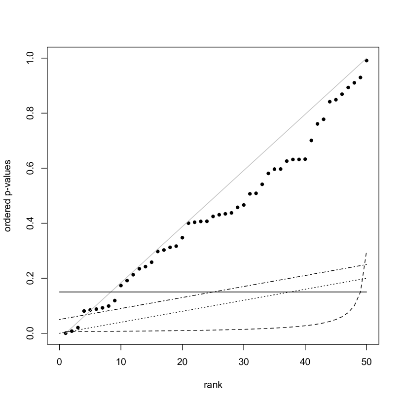
When testing the existence of $m$ potential effects, it is customary to compute an individual p-value $p_{i}$ for each null hypothesis $H_{0i},\,i=1,\ldots,m$. A true effect tends to have a p-value close to zero, while a null effect has a randomly assigned p-value between $0$ and $1$. Let $m=m_{0}+m_{1}$ be the decomposition into the number of null effects and true effects, respectively. The plot of the ordered p-values against the rank provides a simple visual check to see whether any effect is present at all. The resulting graph of $p_{(r)}$ vs $r$ for $r=1,\ldots,m$ carves out an non-decreasing sequence of points in the rectangle $[1;m]\times[0;1]$ and should, if no real effect exists, stay close to the diagonal from the lower left corner to the upper right corner of the square. Procedures of higher criticism can be based on a second curve or threshold sequence $t_{r}$, which stays close to the lower edge of the square. If all p-values are above this curve, none of the tests rejects. If any of the p-values are below the threshold curve, there are several possible procedures. We will concentrate on the maximum p-value below the curve. All the tests with p-value smaller or equal to this maximum then reject. Figure 1 illustrates this general idea. If such a procedure is applied, each effect we test is either rejected or not rejected. Table 1 introduces the contingencies that occur.

Figure 1: The plot shows for $m=50$ tests the ordered p-values plotted against the rank. Besides the diagonal, three other curves are shown, which have appeared in the literature as thresholds. They are the constant threshold $t_{r}=0.15$ (solid line), the proportional threshold $t_{r}=0.004r$ (dotted line) and the curved threshold $t_{r}=0.3/(m+1-r)$ (dashed curve). With the constant, 9 tests reject, with the proportional, 1 test rejects and with the curved, 2 tests reject. In addition a linear threshold $t_{r}=0.05+0.004r$ is shown.

Hypotheses	not rejected	rejected	Total
True	TN	FP	$m_{0}$
False	FN	TP	$m_{1}$
Total	$m-R$	$R$	$m$

Table 1: General outcome of separating $m$ tests into non significant and significant ones. TP, FP denote the number of true, false rejections (true, false positives), respectively. $R$ is the total number of rejections. TN, FN denote the number of true, false non-rejections (true, false negatives), respectively.

If we take the classical meaning of “statistical significance at level $\alpha$” and reject all tests with $p_{(r)}\leq t_{r}=\alpha$, or equivalently $p_{i}\leq\alpha$, the expected number of false rejections is equal to $m_{0}\alpha$. If $m=1000$ and $\alpha=0.05$, we expect around 50 false rejections under the assumption that $m_{1}$ is moderate. In Figure 1, the horizontal threshold has $\alpha=0.15$ and we expect around 7.5 false rejections. The 9 rejections we actually found is close enough to 7.5 to suspect that most or even all the rejections are false positives.

Even though this calculation makes it clear that performing many tests in parallel challenges the classical sense of “statistically significant”, a large number of claims are still published in the scientific literature without a proper control (Benjamini, 2010). To make things worse, the above calculation neglects previously published or unpublished studies that have tested the same or related hypotheses, thus even further increasing the risk of spurious findings.

There is an obvious solution to the dilemma; we can simply replace $t_{r}=\alpha$ by $t_{r}^{\text{Bonf}}=\alpha/m$. If we do this, the expected number of false rejections is less than or equal to $m_{0}\alpha/m\leq\alpha$. Bonferroni (1936) shows that in many circumstances this test also controls another aspect, namely the probability of making one or more false rejections. This stringent error control is one of the recommended solutions to the dilemma of multiplicity, but can only be applied for modest values of $m$, because otherwise the ability to find the real effects of interest vanishes.

More accommodating procedures were investigated. Holm (1979), for example, showed that the curved threshold $t_{r}^{\text{Bonf}}\leq t_{r}^{\text{Holm}}=\alpha/(m+1-r)$, lying along a convex function, provides the same protection. Simes (1986) went even further by considering the proportional choice $t_{r}^{\text{Holm}}\leq t_{r}^{\text{Simes}}=r\alpha/m$. He showed that for independent uniformly distributed p-values this still controls the probability of one or more erroneous rejections. A breakthrough occurred with Benjamini and Hochberg (1995). These authors recognized that it is useful to study the proportional threshold in the context of another error metric, namely the false discovery proportion ${\mathit{FDP}}={\mathit{FP}}/\max(R,1)$. They showed that using the proportional threshold $t_{r}^{\text{Simes}}$ ensures that $\mathbb{E}({\mathit{FDP}})\leq\alpha$ (BH procedure).

In all these examples, the values of the thresholds lie between $\alpha/m$ and $\alpha$. This is reasonable since these two bounds represent the cases of “severe correction” and “no correction”. In this paper, we explore what happens, if the threshold $t_{r}$ satisfies $\alpha/m\leq t_{r}\leq\alpha$ and is non-decreasing, for example, the linear threshold $t_{r}^{\text{linear}}=A+Br$, where $A,B\geq 0$ and $A+B>0$?

2 Main results

If we are willing to contemplate new error metrics, the answer to “what happens with arbitrary thresholds?” has an easy answer. Let the number of rejections be $R$, the largest rank such that $p_{(R)}\leq t_{R}$ (see Fig. 1) and zero if all the p-values are larger than the threshold. We will show that with this threshold,

$$\frac{1}{m}\mathbb{E}\left(1_{\{R>0\}}\frac{{\mathit{FP}}}{t_{R}}\right)\leq 1\,,$$ (1)

which means that a ratio of the number of false positives divided by a positive and non-decreasing function of the total number of rejections is controlled. In order to relate this inequality to familiar results, we consider thresholds of the form

$$t_{r}=s_{r}\alpha/m\,,$$ (2)

where the $0\leq s_{r}\leq m$ is a non-decreasing sequence, which we will call the shape of the threshold, and $\alpha>0$ is an arbitrary tuning constant that controls the severity of the error control. The bigger $\alpha$, the larger the threshold and the larger the number of rejections. With this notation, inequality (1) becomes

$$\mathbb{E}\left(1_{\{R>0\}}\frac{{\mathit{FP}}}{s_{R}}\right)\leq\alpha\,.$$ (3)

For the thresholds we have discussed in Section 1, the inequality (3) yields the results in Table 2.

Name	threshold $t_{r}$	shape $s_{r}$	control
Bonferroni	$\alpha/m$	$1$	$\mathbb{E}(1_{\{R>0\}}{\mathit{FP}})=\mathbb{E}({\mathit{FP}})\leq\alpha$
Holm	$\alpha/(m+1-r)$	$\frac{m}{m+1-R}$	$\mathbb{E}(1_{\{R>0\}}\frac{m+1-R}{m}{\mathit{FP}})\leq\alpha$
BH	$r\alpha/m$	$r$	$\mathbb{E}(1_{\{R>0\}}\frac{{\mathit{FP}}}{R})\leq\alpha$
Linear	$A+Br$	$\frac{m(A+Br)}{\alpha}$	$\mathbb{E}(1_{\{R>0\}}\frac{{\mathit{FP}}}{m(A+BR)})\leq\alpha$

Table 2: The control exerted by using the thresholds discussed in Section 1. The Bonferroni and BH case are well-known, the other two are new. The Holm threshold controls the expected number of erroneous rejections, but multiplied by a weight smaller or equal to 1 that decreases linearly as $R$ increases. The linear and proportional thresholds also control such a weighted expectation, with decreasing weights depending on $R$.

Inequality (3) gives us a clearer understanding of procedures of higher criticism based on thresholding p-values of families of tests. The threshold is meant to capture the p-values belonging to true effects from above. In Fig. 1, such p-values cluster near the bottom left corner, that is, they are small and have low rank. At least this is the situation we have in mind, even though this will not happen if the true effects are not large enough. If we move to the right along the curve of the ordered p-values, the ones belonging to true effects will become rare and the p-values sequence cuts across the threshold.

The proportional thresholds $t_{r}=r\alpha/m$ are ideal in situations where the number of true effects is small and the effects are just barely detectable. In other situations, the number $R$ of detected effects can be large or moderately large and the proportional thresholds will then find a sizable number of false positives and loose their effectiveness. This was our motivation for studying other thresholds. We are, however, interested in threshold shapes $s_{r}$ that grow linearly in $r$ for small values, but sub-linearly for larger values $r$. The prototype is the trimmed threshold $s_{r}^{trunc}=\min(\tau,r)$ for $1\leq\tau\leq m$.

Definition 2.1

Consider an arbitrary non-decreasing threshold $t_{r}=s_{r}\alpha/m$ $(r=1,\ldots,m)$ with non-decreasing shape function $1\leq s_{r}\leq m$. The matched error metric is the penalized false discovery proportion

$$\mathit{pFDP}=\frac{{\mathit{FP}}}{s_{R}}\,,\text{ if }R\geq 1\text{ and }=0\,,\text{ otherwise}\,.$$

We call the expectation of the $\mathit{pFDP}$ the penalized false discovery rate, $\mathrm{pFDR}=\mathbb{E}\left(\mathit{pFDP}\right)$.

In an older version of the manuscript (Meskaldji et al., 2011), we show that with particular cases of the shape function, one can recover a large number of type I error rates that have been introduced in the literature.
Our results are valid for $m\geq 2$ and cover the $\mathrm{pFDR}$ control via step-up procedures under independence, positive dependence and general dependence, as well as the control via weighted procedures (Benjamini and Hochberg, 1997; Genovese et al., 2006). In a weighted procedure, an a priori non-negative weight $w_{i}$ is assigned to each null hypothesis $H_{0i},$ and the raw p-values $p_{i}$ are replaced by the weighted p-values $q_{i}=p_{i}/w_{i}$ if $w_{i}>0$ and $q_{i}=1$ if $w_{i}=0$. A hypothesis of big weight is more easily rejected than a hypothesis of small weight. The weights have to be standardized so that $\sum_{i=1}^{m}w_{i}=m$, which includes $w_{i}\equiv 1$ as a possibility. The threshold can also be interpreted as a weight, albeit one that applies to the rank of the hypothesis as determined by its p-value. If we re-write $p_{(r)}\leq s_{r}\alpha/m$ as $p_{(r)}r/s_{r}\leq r\alpha/m$, we see that the method acts as a weighted BH procedure with weight proportional to $w_{i}\propto s_{\text{rank of hypothesis i}}/\text{rank of hypothesis i}$. Since these weights depend on the p-values, the condition $\sum_{r}^{m}s_{r}/r=m$ does not guarantee the control of the FDR.

3 Discussion, Examples and Simulations

3.1 Relation to the literature

Other studies have proposed threshold sequences different from the horizontal or the proportional, among them Genovese and Wasserman (2002, p. 508 and p. 513), where it is shown that asymptotically the proportional one is optimal in some sense, Finner et al. (2009), who derive an alternative threshold sequence based on asymptotic arguments, and Roquain and Villers (2011), who investigate the operating characteristics of the FDR under an increasing threshold sequence. But none of these papers makes the connection to a generalization of the error metric. Metrics related to ours were introduced in van der Laan et al. (2004) and described in Dudoit and van der Laan (2008, p. 238 and ch. 6, 7). These references consider transformations that involve both ${\mathit{FP}}$ and $R$, while we concentrate on transforming $R$ alone.

3.2 The choice of the threshold sequence

The freedom offered by using any threshold sequence is practical and useful. It gives users the opportunity to choose on a very fine scale between tests that merely provide a screening of a large numbers of potential effects and on the other hand tests that exert a strict control on the number of false discoveries, but have difficulties in finding moderately large true effects.

When applying a procedure that exerts FDR control, we can expect to have ${\mathit{FP}}\approx\frac{m_{0}}{m}\alpha R$ for $m>>1$ (Roquain and Villers, 2011), which means that the number of false effects “discovered” increases as a fraction of the total number of effects found. The Bonferroni procedure satisfies $\mathbb{E}({\mathit{FP}})\leq m\alpha/m=\alpha$, independently of $R$. Since none of the error metrics is superior in all aspects, the users may wish to have several distinct controls achieved by one procedure. On general principles, an ideal procedure is as powerful as possible when it comes to detecting true effects and, at the same time, controls the expected number of false positives. The BH procedure does achieve this for smallish $R$, but at the risk of large values of ${\mathit{FP}}$ when $R$ becomes large. To avoid this, one can add strong control of $\mathbb{E}({\mathit{FP}})$ at a relaxed level $\tau\alpha\;(\tau\geq 1)$ as Hommel and Hoffmann (1987) guarantees. In the context of penalized false discovery procedures, the truncated linear threshold, $t_{r}^{\text{trunc}}=s_{r}^{\text{trunc}}\alpha/m$, with shape function $s_{r}^{\text{trunc}}=\min(\tau,r)$ provides a solution. The corresponding step-up procedure with threshold sequence $t_{r}^{\text{trunc}}$ controls the FDR to be less than $\alpha$ and controls $\mathbb{E}({\mathit{FP}})$ to be less than $\tau\alpha$. We might call this type of control the truncated FDR. This is an appropriate choice, if the number $m$ of hypotheses being tested is very large. Applications include functional magnetic resonance images in the neuroscience as well as many genomic or other “omic” studies (Meskaldji et al., 2015; Meskaldji et al., 2013).

Note that the truncated FDR could be written as

$$\mathbb{E}\left(\frac{{\mathit{FP}}}{s_{R}^{\text{trunc}}}\right)=\mathbb{E}\left(\frac{{\mathit{FP}}}{\min(\tau,R)}\right)=\max\left[\mathbb{E}\left(\frac{{\mathit{FP}}}{R}\right),\mathbb{E}\left(\frac{{\mathit{FP}}}{\tau}\right)\right]\\ =\max\left[{\mbox{FDR}},\frac{1}{{\tau}}\mathbb{E}\left({\mathit{FP}}\right)\right]\,.$$

A similar criterion (with smooth transition) is obtained by minimizing the expected number of false positives while simultaneously controlling the false discovery rate. This leads to a family of mixed error rates indexed by $0<\epsilon<1$

$$\text{MER}_{\epsilon,\tau}=\epsilon\mathbb{E}({\mathit{FP}}/\tau)+(1-\epsilon)\mathbb{E}({\mathit{FP}}/R)\,,$$

where $\epsilon$ tunes the transition between the two controls. To derive a step-up procedure that controls the MER, we use Propositions 4.1 and 4.2. We have

$$\text{MER}_{\epsilon,\tau}=\mathbb{E}\left[{\mathit{FP}}\left(\frac{R}{\epsilon R/\tau+(1-\epsilon)}\right)^{-1}\right]\,,$$

which we recognize as a pFDR with shape sequence

$$s_{r}^{\epsilon,\tau}=\frac{r}{\epsilon r/\tau+(1-\epsilon)}\,.$$

This sequence has a roughly linear rise for small $r$ and then flattens out to reach the horizontal asymptote $r=\tau/\epsilon$. Control at level $\alpha$, when $m$ hypotheses are tested, is obtained by the thresholds

$$t_{r}^{\epsilon,\tau}=s_{r}^{\epsilon,\tau}\alpha/m=\frac{r}{\epsilon r/\tau+(1-\epsilon)}\alpha/m\,.$$

3.2.1 Simulations

Figure 2: Behavior of the gain $\mathcal{G}_{1}$ and the gain $\mathcal{G}_{2}$ of different procedures compared to BH, as a function of the price $\lambda$. Here we show the difference between the gain function of each procedure and the one corresponding to the BH procedure. The number of tests is $m=1000$ and the number of false hypotheses is $m_{1}=100$. The effect size $\Delta$ is either 1,2, or 3. The curves show the simulated gains minus the gain of the BH procedure (zero line), Bonferroni (continuous), truncated linear with $\tau=5$ (small dashes), $\tau=20$ (small-big dashes) and $\tau=100$ (large dashes).

Figure 3: Behavior of the gain $\mathcal{G}_{1}$ and the gain $\mathcal{G}_{2}$ of different procedures compared to BH, as a function of the price $\lambda$. Here we show the difference between the gain function of each procedure and the one corresponding to the BH procedure. The number of tests is $m=1000$ and the number of false hypotheses is $m_{1}=50$. The effect size $\Delta$ is either 1,2, or 3. The curves show the simulated gains minus the gain of the BH procedure (zero line), Bonferroni (continuous), truncated linear with $\tau=5$ (small dashes), $\tau=20$ (small-big dashes) and $\tau=100$ (large dashes).

Figure 4: Behavior of the gain $\mathcal{G}_{1}$ and the gain $\mathcal{G}_{2}$ of different procedures compared to BH, as a function of the price $\lambda$. Here we show the difference between the gain function of each procedure and the one corresponding to the BH procedure. The number of tests is $m=10000$ and the number of false hypotheses is $m_{1}=1000$. The effect size $\Delta$ is either 1,2, or 3. The curves show the simulated gains minus the gain of the BH procedure (zero line), Bonferroni (continuous), truncated linear with $\tau=5$ (small dashes), $\tau=20$ (small-big dashes) and $\tau=100$ (large dashes).

Figure 5: Behavior of the gain $\mathcal{G}_{1}$ and the gain $\mathcal{G}_{2}$ of different procedures compared to BH, as a function of the price $\lambda$. Here we show the difference between the gain function of each procedure and the one corresponding to the BH procedure. The number of tests is $m=10000$ and the number of false hypotheses is $m_{1}=500$. The effect size $\Delta$ is either 1,2, or 3. The curves show the simulated gains minus the gain of the BH procedure (zero line), Bonferroni (continuous), truncated linear with $\tau=5$ (small dashes), $\tau=20$ (small-big dashes) and $\tau=100$ (large dashes).

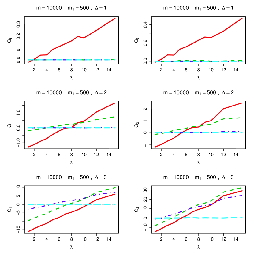
To complete this section, we present some simulations that demonstrate the advantage of using the truncated FDR. We compare three multiple testing procedures: the Bonferroni procedure, the most stringent, the BH procedure, the least stringent, and the truncated linear procedure which bridges the gap between theses two extremes. We restrict our simulations to the case of shifted Gaussians, that is, if the null hypothesis is true, the test statistic follows a Gaussian law with expectation 0 and variance 1, while false hypotheses are Gaussians with expectation $\Delta>0$ and variance 1. The values of the test statistics are independent. We will call $\Delta$ the effect.

The general goal of any multiple testing procedure consists in making ${\mathit{TP}}$ large while keeping ${\mathit{FP}}$ small. These two types of rejections are opposites of each other, but asymmetrical opposites. Among multiple testing procedures that satisfy a given error control, the ones that reject a maximal number of hypotheses are preferred. This is often the only measure of optimality that is investigated. We consider instead a simple monetary utility function with expected value

$$\mathcal{G}_{1}=\mathbb{E}({\mathit{TP}})-\lambda\mathbb{E}({\mathit{FP}})\,,$$ (4)

in which each true discovery leads to a gain of 1 and each false discovery to a loss of $\lambda\geq 1$. This approach might be unfamiliar to statisticians, who are used to maximizing power under control of the false rejections, but it can be shown that the two are closely related in the Neyman-Pearson context. Our criterion allows a mixture of different error rates and will pick the one best adapted to $\lambda$. In the philosophy of multiple testing, $\lambda>1$, because the subsequent investigation of any discovery is expensive and being on the wrong track may be a costly mistake.

It is stated in Benjamini and Hochberg (1995) that the BH procedure is optimal in the sense that under the FDR control, it maximizes the number of rejections. In situations where $m_{1}$ and the effect are large, the number of true rejections is expected to be large. To maximize the number of rejections, counting both true and false, the BH procedure can be expected to add rejections of null hypotheses, even though the corresponding p-values are no longer small and we in fact reject a sizable proportion of false ones.
Another monetary utility function to counteract such behavior has expected value

$$\mathcal{G}_{2}=\mathbb{E}({\mathit{TP}})-\lambda\mathbb{E}(1+2+\ldots+{\mathit{FP}})=\mathbb{E}({\mathit{TP}})-\frac{\lambda}{2}\left(\mathbb{E}({\mathit{FP}})+\mathbb{E}({\mathit{FP}}^{2})\right)\,,$$ (5)

where the loss due to a false discovery increases with each false discovery. This gain function does not only consider the expected number of false positive, but also its variance.

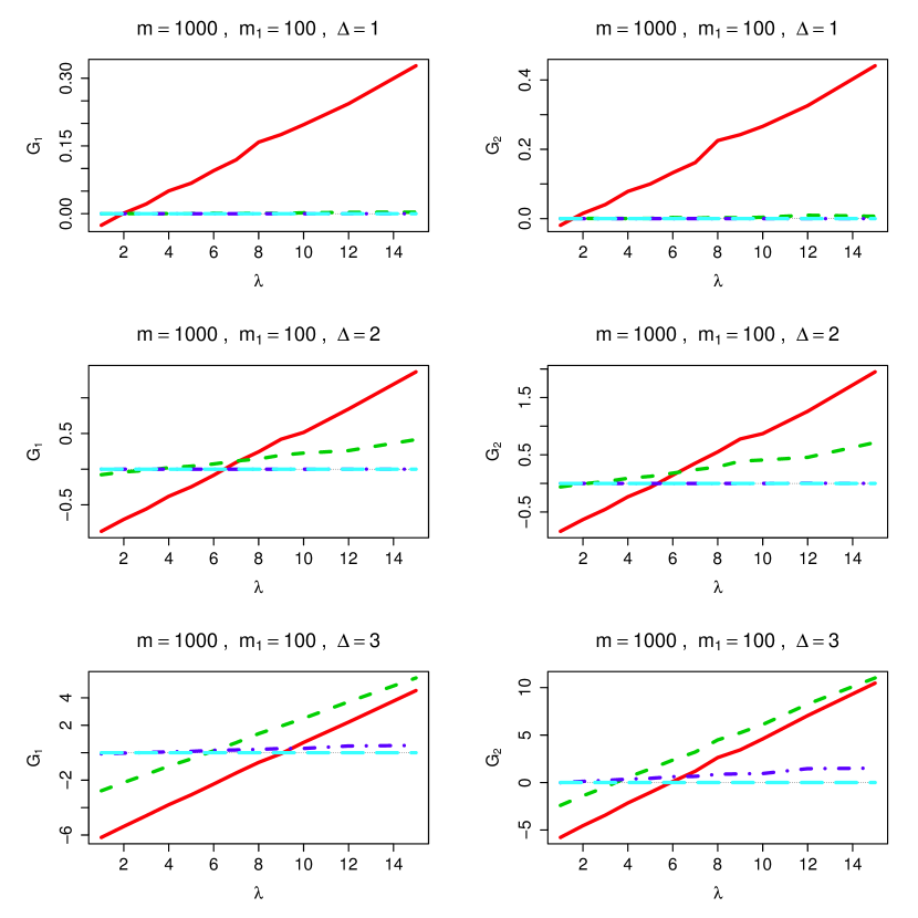
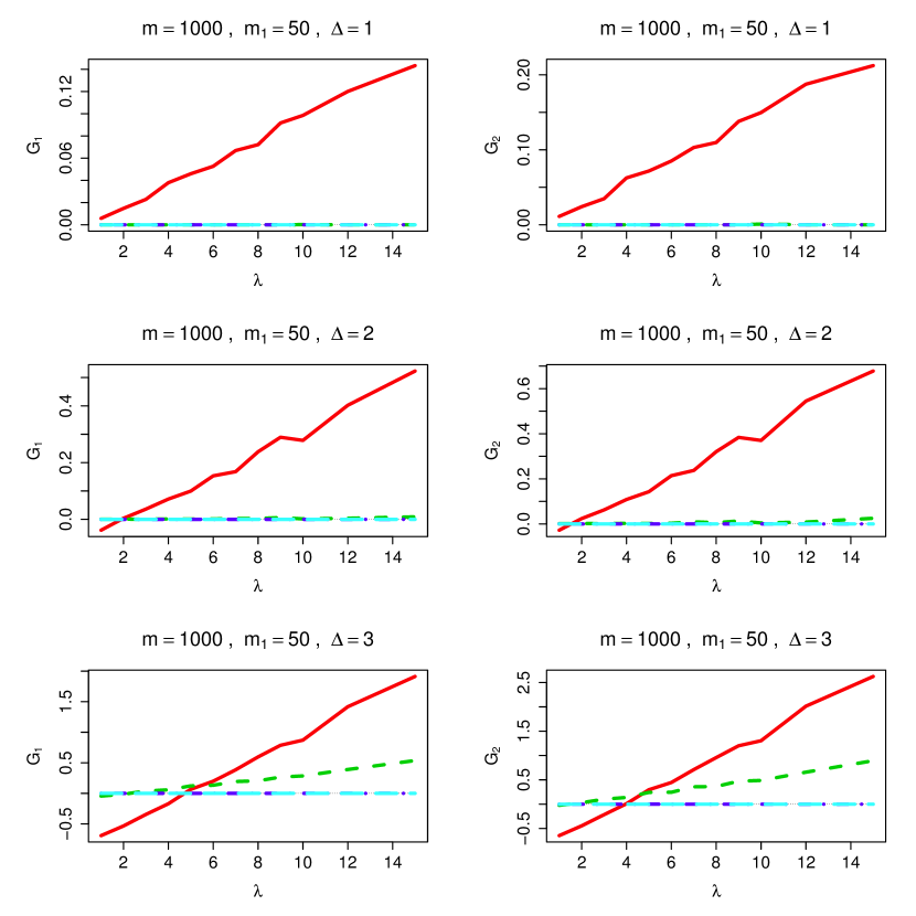
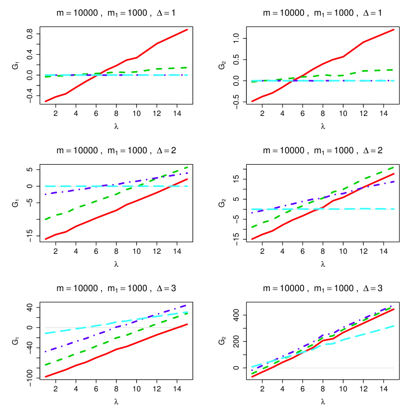
We compare the gain functions of different procedures to the of the BH procedure, as a function of the price $\lambda$. Figures 2, 3, 4 and 5 show the difference between the gain functions of the Bonferroni procedure, the truncated linear procedure with different values of $\tau$ (5, 20 and 100), and the BH gain functions, for various choices of the number of tests $m$, of the number of false null hypotheses $m_{1}$ and of the effect $\Delta$. Any curve above zero indicates that the BH procedure is worse than the corresponding competing procedure, and vice versa for below zero. For both gains, the truncated linear procedures compensate a considerable part of the power lost by the Bonferroni procedure without committing a large number of false positives. Both the truncated linear and the Bonferroni procedure are much more stable in terms of control of false positives. The BH procedure seems to be appropriate only when the price $\lambda$ of a false discovery is small. In some cases, the BH procedure is optimal only when $\lambda=1$, which corresponds to the case where a false rejection and a false acceptance of a null hypothesis are considered to be of equal harm.

As expected, the shortcomings of the BH are very pronounced for large $m$. In the sparse case ($m_{1}=500$), the BH procedure is not much more powerful than the other procedures when the raw effect is weak ($\Delta=1$). When the effect becomes moderate ($\Delta=2$) or strong ($\Delta=3$), the truncated procedures behave better than both the BH and the Bonferroni procedure for reasonable values of the price $\lambda$. When the number of alternative increases ($m_{1}=1000$ or $2000$), the performances of the truncated methods are still good. However, the BH procedure shows a marked performance instability, especially for $m_{1}=2000$ and $\Delta=3$.
The simulations suggest the use of the truncated linear with a value of $\tau$ that is situated between 20% and 50% of $\sqrt{m}$.

3.2.2 Examples

Gene expression levels of $m=35512$ genes were measured in two tissues of male mice who were fed either a normal diet or a high-fat diet (Hasenfuss et al., 2014). We first consider an initial exploration of the gene-by-gene comparison of the two tissues (strong difference). Two-sample t-tests were performed to compare the expression levels in the muscle versus the liver. The results are given as two-sided p-values, one for each gene. The left-hand panel of Figure 6 shows that a large majority of the genes exhibit a significant differential effect between the two tissues. The Bonferroni procedure with $\alpha=0.05$ finds $21020$ differentially expressed genes, whereas the BH procedure with $\alpha=0.05$ identifies $28436$ such genes. Under Bonferroni we stop reporting positives early, in order to avoid the declaration of false discoveries. Under BH, assuming that $m_{1}=29000$, one would expect approximately $261$ falsely identified genes, namely $0.05\times 28436\times(6512/35512)$, whereas the Bonferroni procedures has an approximate expectation of $0.05\times(6512/35512)=0.009$ false positives.

It is evident, that these two procedures cannot be compared directly. If we were to match the approximate expected number of false discoveries, the Bonferroni procedure would need $\alpha=1422$, rather than $\alpha=0.05$ and this procedure detects $28437$ significances, that is, the two threshold sequences meet the ordered p-values almost at the same point. The left-hand panel of Fig. 6 shows these two threshold sequences. The truncated procedure with $\tau=1422$, in which we decide to apply FDR control up to a certain level and then switch to Bonferroni control would, of course, give exactly the same result. This illustrates a fact pointed out by Genovese and Wasserman (2002), namely that the value where the threshold sequence crosses the ordered p-values is the only aspect of interest when investigating asymptotic error rates of the threshold sequence.

Commenting on this first example, we can say that when many null hypotheses are rejected, the BH procedure is a questionable choice for performing multiple testing. By definition of the control metric, a large number of rejections means that a large number of false rejections are tolerated. The Bonferroni procedure with $\alpha=0.05$ tolerates none or at most a few false discoveries, but can only achieve this feat by limiting the reported number of significances. Among these first $21000$ positives the fraction of false ones is negligible. The BH procedure with the same $\alpha=0.05$ has roughly an additional $7500$ rejections. Among these, we estimate that $261/7500=3.5\%$ are false. The local rate of false discoveries increases when we only consider the last 7500 rejections.

Figure 6: Ordered p-values corresponding to gene expression level of $m=35512$ genes in two tissues of male mice, some fed a healthy diet, some a high-fat diet. In the left-hand panel the p-values are obtained from gene-by-gene comparison between muscle and liver, both diets confounded. The right-hand panel shows the p-values obtained when comparing the two diets in liver cells.

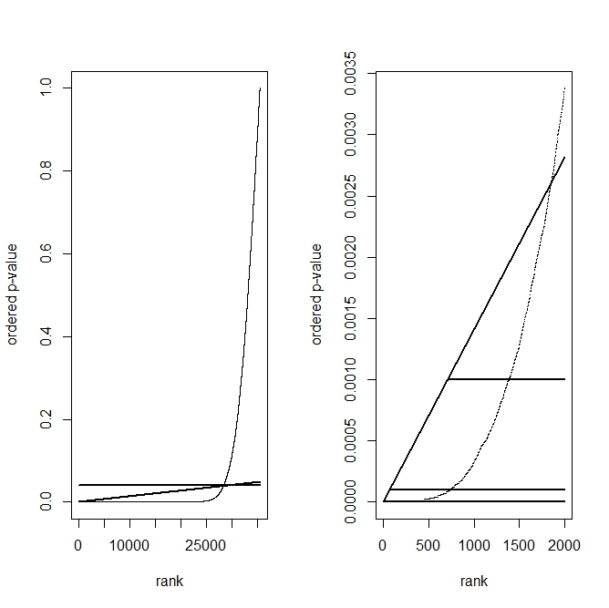
As a second example, the right-hand panel of Figure 6 shows the (rounded) p-values one obtains when comparing the two diets in the liver. In this case, we only take the data from one tissue and we thus have only half the previous number of observations. Only a few of the $35512$ genes are differentially expressed, that is, the effect is weaker than in the first example, and because of this, we only show the smallest $2000$ p-values. The superposed curves show the BH threshold sequence with $\alpha=0.05$, the Bonferroni threshold with $\alpha=0.05$ and truncated threshold sequences with $\tau=71$ ($\tau\approx 38\%$ of $\sqrt{m}$) and $\tau=710$ ($\tau\approx 380\%$ of $\sqrt{m}$). The FDR control results in $1853$ discoveries, whereas the Bonferroni procedure discovers $353$ genes. The truncated thresholds result in $737$ and $1386$ rejections, respectively. This second example shows, in a case where the effect is moderate, the advantage of using the truncated threshold over the Bonferroni procedure. Up to a certain number of discoveries, we accept the FDR control and then switch to a relaxed Bonferroni. If the effect becomes sparse and a truncated threshold is used, the up-crossing of the ordered p-values may happen in the linearly increasing part of the threshold sequence. In this case, the truncated threshold behaves similarly to the FDR procedure and is able to detect sparse signals, whereas the Bonferroni procedure will miss them. At the same time, it offers better control.

These examples illustrate how to use a truncated linear procedure in order to increase the power considerably, but without incurring a punishingly high expected number of false rejections. The optimal choice of the $\tau$ parameter depend on the price that the researcher is willing to pay when committing a false discovery and on the (unknown) effect sizes.

4 Results, proofs, and further discussions

The theory developed in Blanchard and Roquain (2008) can be adapted to our error rate. Three of their lemmas form the basis, together with the concept of self consistency.

Any step-up procedure is such that the rejection set satisfies ${\mathcal{R}}=\{i\in I=\{1,\ldots,m\}:p_{i}\leq T\}$, where $T$ is an upper bound which usually depends on the p-values $p_{1},\ldots,p_{m}$. To prove control, we need to bound

$$\mathrm{pFDR}(T)= \mathbb{E}\left[\frac{{\mathit{FP}}}{s_{R}}{\mathbf{1}\left\{R>0\right\}}\right]$$

$$= \sum_{i\in I_{0}}\mathbb{E}\left[\frac{{\mathbf{1}\left\{p_{i}\leq T\right\}}}{s_{R}}{\mathbf{1}\left\{R>0\right\}}\right],$$ (6)

where $I_{0}={\{i\in I\text{ such that }H_{i}\text{ is true}\}}$. The family of threshold sequences $\Gamma:I\times\mathbb{R}^{+}\mapsto\mathbb{R}^{+}$ of the form

$$\Gamma(i,r)=\frac{\alpha}{m}w_{i}s_{r}\,,$$

with $i$ denoting the null hypothesis and $r$ the rank of its p-value covers all cases of interest to us. It takes account of the weights $\{w_{i},i\in I\}$ and the shape $s_{r}$. Such a threshold sequence leads to a step-up procedure that satisfies

$${\mathcal{R}}\subset\{i\in I\;|\;p_{i}\leq\Gamma(i,R)\}\,,$$

where ${\mathcal{R}}$ is the set of rejections. This holds for all $R$ and is called the self-consistency condition.

4.1 Control of the $\mathrm{pFDR}$ under independence

Proposition 4.1

Assume that the $p$-values $p_{1},\ldots,p_{m}$ are independent random variables and that non-negative weights $w_{1},\ldots,w_{m}$ are given. It follows that the step-up procedure with threshold sequence $t_{r}=s_{r}\alpha/m$ (see Def. 2.1) applied to $q_{1}=p_{1}/w_{1},\ldots,q_{m}=p_{m}/w_{m}$ ($q_{i}=1$ if $w_{i}=0$), satisfies

$$\mathrm{pFDR}=\mathbb{E}({\mathit{FP}}/s_{R})\leq\alpha/m\sum_{i=1}^{m}w_{i}\,.$$

Proof 4.1

Denote by $\mathbf{p}_{-i}$ the set of $p$-values $\{p_{j}\;|\;j\neq i\}$. From (6) and using the self-consistency, we have

$$\mathrm{pFDR}(R) =\sum_{i\in I_{0}}\mathbb{E}\left[\frac{{\mathbf{1}\left\{p_{i}/w_{i}\leq s_{R}\alpha/m\right\}}}{s_{R}}\right]$$

$$\leq\sum_{i\in I_{0}}\mathbb{E}\left[\mathbb{E}\left[\frac{{\mathbf{1}\left\{p_{i}\leq\frac{\alpha}{m}w_{i}s_{R(\mathbf{p})}\right\}}}{s_{R(\mathbf{p})}}\middle|\mathbf{p}_{-i}\right]\right]$$

$$\leq\frac{\alpha}{m}\sum_{i\in I_{0}}w_{i}\,,$$

where we used the fact that given $\mathbf{p}_{-i}$, $p_{i}$ is stochastically lower bounded by a uniform distribution in the independent case. By case (i) of the Lemma 3.2 of Blanchard and Roquain (2008) we obtain the result if we set $U=p_{i},\;g(U)=s(R(\mathbf{p}_{-i},U))$ and $c=\frac{\alpha}{m}w_{i}$. Note that $g(s_{R(\mathbf{p}_{-i},U)})$ is non increasing in $U$ since $s_{r}$ is non-decreasing and $R$ is non-increasing in $U$.

4.2 Control of the $\mathrm{pFDR}$ under positive dependence

Proposition 4.2

Assume that the $p$-values $p_{1},\ldots,p_{m}$ are positively dependent (positively regression dependent on a subset as in Benjamini and Yekutieli (2001)) random variables and that non negative weights $w_{1},\ldots,w_{m}$ are given. It follows that the step-up procedure with threshold sequence $t_{r}=s_{r}\alpha/m$ (see Def. 2.1) applied to $q_{1}=p_{1}/w_{1},\ldots,q_{m}=p_{m}/w_{m}$ ($q_{i}=1$ if $w_{i}=0$), satisfies

$$\mathrm{pFDR}=\mathbb{E}({\mathit{FP}}/s_{R})\leq\alpha/m\sum_{i=1}^{m}w_{i}\,,$$

where $R$ denotes the number of rejections.

Proof 4.2

By case (ii) of the Lemma 3.2 of Blanchard and Roquain (2008), with $U=p_{i}$, $V=s(R)$ and $c=\frac{\alpha}{m}w_{i}$, the result follows.

4.3 Control of the $\mathrm{pFDR}$ under any dependence structure

Under arbitrary dependence of the p-values, an additional correction to the thresholds has to be performed. Let $\nu$ be a probability distribution on $(0,\infty)$ and define for $r>0$

$$\xi(r)=\int_{0}^{r}ud\nu(u)\,.$$ (7)

We call the $\xi$ function the reshaping function. It was introduced in Blanchard and Roquain (2008), who called $\xi(r)$ shape function, because they studied only the case of proportional thresholds.

Proposition 4.3

Let $p_{1},\ldots,p_{m}$ be the p-values computed for the $m$ null hypotheses. Non-negative weights $w_{1},\ldots,w_{m}$ are given. Let $\xi(r)$ be as described above. It follows that the step-up procedure with threshold sequence $t_{r}=\xi(s_{r})\alpha/m$ applied to $q_{1}=p_{1}/w_{1},\ldots,q_{m}=p_{m}/w_{m}$ ($q_{i}=1$ if $w_{i}=0$), satisfies

$$\mathrm{pFDR}=\mathbb{E}({\mathit{FP}}/s_{R})\leq\sum_{i=1}^{m}w_{i}\alpha/m\,.$$

Proof 4.3

By case (iii) of the Lemma 3.2 of Blanchard and Roquain (2008) with $U=p_{i}$, $V=s(R)$ and $c=w_{i}\alpha/m$ the result follows.

4.4 Discussion on reshaping

The reshaping function $\xi(r)=r/(1+1/2+\ldots+1/m)$ is obtained for the probability measure $\nu$ that puts point mass proportional to $1/r$ on $r=1,\ldots,m$. The corresponding threshold sequence for the general dependence case (Proposition 4.3) is

$$t_{r}=s_{r}\alpha/(m(1+1/2+\ldots+1/m))\,.$$ (8)

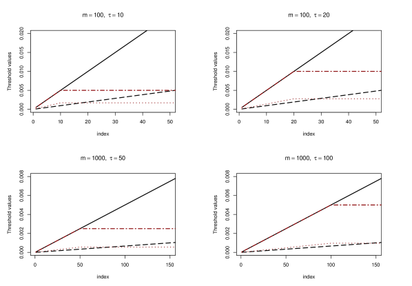
The corresponding step-up testing procedure is a penalized version of the procedure proposed in Benjamini and Yekutieli (2001). If we instead take $\nu$ as the probability measure with point mass proportional to $1/1,\,1/2,\ldots$ with support $\{1,2,\ldots,\tau\}$, the reshaping function truncates, because it is equal to

$$\xi(r)=r\left(\sum_{i=1}^{\tau}\frac{1}{i}\right)^{-1}\text{ for }r\leq\tau\text{ and }\xi(r)=\xi(\tau)\text{ for }r>\tau\,.$$

The corresponding threshold sequence is

$$s(r)^{\text{trunc}}\alpha\Big{/}\left(m\sum_{i=1}^{\tau}\frac{1}{i}\right)\,,$$

which exceeds (8) for $r\leq{\lfloor}{\tau\sum_{i=1}^{m}\frac{1}{i}/\sum_{i=1}^{\tau}\frac{1}{i}}{\rfloor}$. This test thus increases the power in some situations even though it exerts a provably stricter control (see Figure 7). A particular case is $\tau=1$, where $\xi(r)\equiv 1$, and the threshold sequence is $\alpha/m$, that is, the Bonferroni procedure.

Blanchard and Roquain (2008) propose other reshaping functions for the FDR case and comment on their use

Figure 7: Examples of threshold sequences for different values of $m$ and $\tau$. The BH procedure (continuous line) and the truncated linear procedure (big/small dashes), both for independent and positively dependent tests. The modified BH thresholds as described in Benjamini and Yekutieli (2001) (dashes) and the modified truncated linear thresholds as described in the Results section (points), both for the distribution free case.

5 Further Results

In addition to the freedom of choice of error rate, the duality that exists between the error rate and the threshold sequence $t_{r}=s_{r}\alpha/m$ together with the reshaping function $\xi(r)$, brings new perspectives to the field of multiple testing procedures and reveals new interesting results. In this section, we give some examples of corollaries and applications of our results.

5.1 Relation between error rates based on expectation
or on tail probabilities

Define the penalized false exceedence rate ($p\text{FER}$) as

$$p\text{FER}_{q}=\mathbb{P}\left(\frac{\text{FP}}{s_{R}}>q\right)\,.$$

By Markov’s inequality

$$p\text{FER}_{q}=\mathbb{P}\left(\frac{\text{FP}}{s_{R}}>q\right)\leq\alpha\Rightarrow\mathbb{E}\left(\frac{\text{FP}}{q\,s_{R}}\right)\leq\alpha\,,$$

from which it follows that the threshold sequence $qs_{r}\alpha/m$ provides conservative control of this error rate, under independence (Theorem 4.1) or positive dependence (Theorem 4.2). Under general dependency structure, we replace $qs_{R}$ by $\xi(qs_{R})$ (see Lemma 4.3). In an older version of the manuscript (Meskaldji et al., 2011), we proposed step-down procedure that tightly controls the pFER, under different assumptions.

An interesting choice is $q=0.5$, in which case the $p\text{FER}_{q}$ becomes the median of $\mathit{FP}/s_{R}$ and we note that in order to achieve control, we simply have to halve $\alpha$. Consequently, if we wish to control the median of the FDP at level $\alpha$, we can use the BH procedure with $\alpha/2$.

5.2 Asymptotics

Hochberg’s procedure is a step-up procedure with Holm’s threshold sequence $t_{r}=\alpha/(m-r+1)$. If we factor out an $\alpha/m$, the shape is seen to be $s_{r}=m/(m-r+1)$. Our results show that Hochberg’s procedure controls

$$\mathbb{E}\left(\frac{\mathit{FP}}{m}(m-R+1)\right)\approx{\mathbb{E}({\mathit{FP}})}\text{ (for large }m)\,,$$

both under independence and positive dependence.

Another example of this type is the asymptotic control of the optimal rejection curve (ORC) introduced by Finner et al. (2009), which controls asymptotically the FDR. We give here a simple proof of that control. The ORC threshold sequence is $t_{r}=r\alpha/(m-r(1-\alpha))$, which equals 1, when $r=m$ and thus has $R=m$. With a slight modification it can be used in practice. When we factor out $\alpha/m$ we obtain $s_{r}=rm/(m-r(1-\alpha))$ and we can conclude that the modified threshold controls the expectation

$$\mathbb{E}\left(\frac{\mathit{FP}}{R}(1-R/m(1-{\alpha}))\right)\to\text{FDR}\text{ as }m\to\infty\,.$$

This result is valid under independence and positive dependence.

5.3 Assumption weakening

For a step-up procedure associated with a specific threshold sequence, one can find different error rates controlled by this procedure under different assumptions on the dependence structure of the p-values. The proportional threshold $t_{r}=r\alpha/m$, for example, is obtained from $\alpha\xi(s_{r})/m$ when $\xi(r)$ is the inverse of the shape sequence $s_{r}$, that is, $\xi(s_{r})=r$. This shows that the BH procedure controls the quantity

$$\mathbb{E}\left[\frac{{\mathit{FP}}}{s_{R}}\right]=\mathbb{E}\left[\frac{{\mathit{FP}}}{\xi^{-1}(R)}\right]$$

at level $\alpha$ under any distribution of the p-values and for an arbitrary choice of $\xi(r)$ or the shape sequence $s_{r}$. We are thus able to determine the error rate that is under control if the independence or positive dependence assumption is violated. This result is obvious for a linear $\xi(r)$ such as $\xi(r)=r/\sum_{i=1}^{m}\frac{1}{i}$, in which case

$$\xi^{-1}(r)=r\sum_{i=1}^{m}\frac{1}{i}=s_{r}\,.$$

The BH procedure, no matter the dependence structure of the p-values, controls

$$\mathbb{E}\left({\mathit{FP}}/\left(R\sum_{i=1}^{m}\frac{1}{i}\right)\right)\leq\alpha\,,$$

which immediately leads to

$$\mathbb{E}\left({\mathit{FP}}/R\right)\leq\alpha\sum_{i=1}^{m}\frac{1}{i}\approx\alpha\,\log(m)\,.$$

Our results thus inter-relate different error rates and conditions on the dependence structures of p-values by the relation

$$t_{r}=\xi(s_{r})\alpha/m\equiv\tilde{s}_{r}\alpha/m,\text{for }r=1,\ldots,m.$$

References

- Benjamini (2010) Benjamini, Y. (2010). Simultaneous and selective inference: Current successes and future challenges. Biometrical Journal 52(6, SI), 708–721.
- Benjamini and Hochberg (1995) Benjamini, Y. and Y. Hochberg (1995). Controlling the false discovery rate: a practical and powerful approach to multiple testing. Journal of the Royal Statistical Society. Series B. Methodological 57(1), 289–300.
- Benjamini and Hochberg (1997) Benjamini, Y. and Y. Hochberg (1997). Multiple hypotheses testing with weights. Scandinavian Journal of Statistics 24(3), 407–418.
- Benjamini and Yekutieli (2001) Benjamini, Y. and D. Yekutieli (2001). The control of the false discovery rate in multiple testing under dependency. The Annals of Statistics 29(4), 1165–1188.
- Blanchard and Roquain (2008) Blanchard, G. and E. Roquain (2008). Two simple sufficient conditions for FDR control. Electronic Journal of Statistics 2, 963–992.
- Bonferroni (1936) Bonferroni, C. E. (1936). Teoria statistica delle classi e calcolo delle probabilità. Pub. del R Ist. Sup. di Sci. Eco. e Com. di Fir. 8, 3–62. Bonferroni adjustment for multiple statistical tests using the same data.
- Dudoit and van der Laan (2008) Dudoit, S. and M. J. van der Laan (2008). Multiple testing procedures with applications to genomics. Springer Series in Statistics. New York: Springer.
- Finner et al. (2009) Finner, H., T. Dickhaus, and M. Roters (2009). On the false discovery rate and an asymptotically optimal rejection curve. The Annals of Statistics 37, 596–618.
- Genovese and Wasserman (2002) Genovese, C. and L. Wasserman (2002). Operating characteristics and extensions of the false discovery rate procedure. Journal of the Royal Statistical Society: Series B (Statistical Methodology) 64, 499–517.
- Genovese et al. (2006) Genovese, C. R., K. Roeder, and L. Wasserman (2006). False discovery control with p-value weighting. Biometrika 93(3), 509–524.
- Hasenfuss et al. (2014) Hasenfuss, S. C., L. Bakiri, M. K. Thomsen, E. G. Williams, J. Auwerx, and E. F. Wagner (2014). Regulation of steatohepatitis and PPARγ signaling by distinct AP-1 dimers. Cell Metabolism 19(1), 84–95.
- Holm (1979) Holm, S. (1979). A simple sequentially rejective multiple test procedure. Scandinavian Journal of Statistics. Theory and Applications 6(2), 65–70.
- Hommel and Hoffmann (1987) Hommel, G. and T. Hoffmann (1987). Controlled uncertainty. In P. Bauer, G. Hommel, and E. Sonnemann (Eds.), Multiple Hypotheses Testing, pp. 154–161. Springer, Heidelberg.
- Meskaldji (2013) Meskaldji, D.-E. (2013). Multiple Comparison Procedures for Large Correlated Data with Application to Brain Connectivity Analysis. Ph. D. thesis, Ecole Polytechnique Fédérale de Lausanne.
- Meskaldji et al. (2013) Meskaldji, D.-E., E. Fischi-Gomez, A. Griffa, P. Hagmann, S. Morgenthaler, and J.-P. Thiran (2013). Comparing connectomes across subjects and populations at different scales. NeuroImage 80(0), 416 – 425. Mapping the Connectome.
- Meskaldji et al. (2011) Meskaldji, D.-E., J.-P. Thiran, and S. Morgenthaler (2011, dec). A comprehensive error rate for multiple testing. ArXiv e-prints 1112.4519.
- Meskaldji et al. (2015) Meskaldji, D.-E., L. Vasung, D. Romascano, J.-P. Thiran, P. Hagmann, S. Morgenthaler, and D. V. D. Ville (2015). Improved statistical evaluation of group differences in connectomes by screening–filtering strategy with application to study maturation of brain connections between childhood and adolescence. NeuroImage 108(0), 251 – 264.
- Roquain and Villers (2011) Roquain, E. and F. Villers (2011). Exact calculations for false discovery proportion with application to least favorable configurations. The Annals of Statistics 39, 584–612.
- Simes (1986) Simes, R. J. (1986). An improved Bonferroni procedure for multiple tests of significance. Biometrika 73(3), 751–754.
- van der Laan et al. (2004) van der Laan, M. J., S. Dudoit, and K. S. Pollard (2004). Augmentation procedures for control of the generalized family-wise error rate and tail probabilities for the proportion of false positives. Statistical Applications in Genetics and Molecular Biology 3, Art. 15, 27 pp. (electronic).