Tracking interacting dust: comparison of tracking and state estimation techniques for dusty plasmas

Abstract

When tracking a target particle that is interacting with nearest neighbors in a known way, positional data of the neighbors can be used to improve the state estimate. Effects of the accuracy of such positional data on the target track accuracy are investigated in this paper, in the context of dusty plasmas. In kinematic simulations, notable improvement in the target track accuracy was found when including all nearest neighbors in the state estimation filter and tracking algorithm, whereas the track accuracy was not significantly improved by higher-accuracy measurement techniques. The state estimation algorithm, involving an extended Kalman filter, was shown to either remove or significantly reduce errors due to “pixel-locking”. It is concluded that the significant extra complexity and computational expense to achieve these relatively small improvements are likely to be unwarranted for many situations.For the purposes of determining the precise particle locations, it is concluded that the simplified state estimation algorithm can be a viable alternative to using more computationally-intensive measurement techniques.

1 INTRODUCTION

Dusty, or complex, plasmas consist of a low-density neutral/ion/electron plasma containing suspended “dust” – negatively-charged macroscopic particles. Dusty plasmas occur in space as well as in various terrestrial discharges ranging from lightning to industrial applications.[Merlino2004] In more controlled environments, dusty plasmas offer a unique testbed for exploring very complex and fascinating physical processes on a kinematic level. In all cases, precise determination of properties of the dusty plasma is a top priority. In particular, the industrial applications of dusty plasmas could benefit from being able to determine, and subsequently control, physical properties of a dusty plasma.

Many properties of a dusty plasma can be inferred from the behavior of the dust particles, which can be non-invasively observed over time via laser illumination and a digital camera, as in Figure 1 which is used in experiments on Mach cones[Samsonov1999] and shock-waves[Samsonov2004]. The particles acquire a charge due to collisions with ions and electrons in the plasma, causing them to interact with each other and the plasma, with often fascinating results. For example, the dust can form crystalline structures or behave in a liquid-like phase (or exhibit phase transitions[Samsonov2004]), on timescales amenable to observation at the individual particle level. The precision of one’s knowledge of the dust behavior is crucial to the reliability of any conclusions made about physical properties of the system[hadziavdic2006]. There are two ways to improve the precision of determining the dynamics of individual particles: more sophisticated measurements, and information processing. The performance of each are considered in this work.

Determining the tracks of multiple, interacting targets is a non-trivial task. Dust particles are typically observed using a video camera, their locations revealed using computer-based image-processing techniques, and their tracks (connected positions in time) formed using track-association algorithms. Such techniques and algorithms are available in varying levels of sophistication, with commensurate levels of accuracy, precision, resource consumption, etc. That is, more sophisticated techniques typically provide better precision and consume more resources such as time and computer memory. This article considers tracking performance and, specifically, a trade-off between resources and accuracy/precision. Motivation for such considerations comes from the ultimate goal of implementing closed-loop control for such experiments, for which the tracking procedure must be automated.

Previous work on tracking individual dusty plasma particles has been somewhat unsophisticated. A common technique is particle tracking velocimetry (PTV), where the distance and direction of particle travel is obtained from consecutive images and used to aid in linking particle locations into tracks.[Samsonov2000, BoesseAiSR04] This process can be automated, but more can be done. A higher level in sophistication for particle tracking is offered by the Kalman filter,[BarShalom, JFRopaedia] which combines a prediction model with measurements to obtain a recursive state estimation algorithm that can be optimal in the minimum-mean-square-error sense for linear dynamics. A simplified Kalman filter has been used on simulated data in the context of a dusty plasma crystal,[hadziavdic2006] where it was shown to perform very well in many situations. Slightly more sophisticated still is the state-estimation algorithm known as the Extended Kalman filter (EKF)[BarShalom, JFRopaedia], which is considered in this work and will be introduced in Section 3.

Figure 1: Schematic of the dusty plasma experimental setup.[Durniak2010] The dusty plasma is contained wholly within a chamber as shown in (a), with the dust illuminated by a laser sheet and imaged from above by a digital camera as shown in (b).

2 SIMULATED DYNAMICS

Simulating experiments affords this study two primary benefits. It allows for a larger exploration of “parameter space” than might be achievable experimentally in a practical period of time. In addition, it allows for the accuracy of the algorithms to be quantified because the “true” particle locations are known. In the future these algorithms will be developed for and tested on experimental data, so it is important to be as realistic as possible at this early stage. To this end, the parameters and images of recent dusty plasma experiments[Samsonov1999, Samsonov2004] are used as a guide for this work.

Three characteristic length scales of importance for dusty plasmas are the particle radius $R$, the Debye screening length $\lambda_{\mathrm{D}}$ and the inter-particle separation $r$. For the case where $R\ll\lambda_{\mathrm{D}}<r$, the dust particle interactions can be described well[Resendes1998] by a point-charge approximation. Each particle of charge $Q_{\mathrm{d}}$ experiences forces from other particles directly, as well as indirectly via the plasma (such as drag forces due to ion motionmotion of neutrals within the plasma). Under the point-charge approximation, the effective potential experienced by one dust particle (labeled $\jmath$) due to another (labeled $k$) consists of a screened (exponentially decreasing), repulsive Coulomb interaction of the Debye-Hückel/Yukawa form:[Konopka2000]

$$\phi_{\jmath,k}(\vec{r}_{\jmath,k}) = k_{0}Q_{\mathrm{d}}\frac{e^{-r/\lambda_{\mathrm{D}}}}{r}{-\frac{1}{2\lambda_{\mathrm{D}}}}{}\hat{r}_{\jmath,k}.$$ (1)

Here $k_{0}=1/(4\pi\varepsilon_{0})$ is Coulomb’s constant, the plasma screening distance is the Debye length ($\lambda_{\mathrm{D}}$), and the particles are separated by $\vec{r}_{\jmath,k}=r\hat{r}_{\jmath,k}$ (note that this separation is time-varying). Assuming a circular two-dimensional geometry (no angular variation), and defining $\tilde{r}\equiv r/\lambda_{\mathrm{D}}$, yields the effective force between two interacting dust particles (the gradient of the potential) to be

$$F(\vec{r}_{\jmath,k})=\frac{k_{0}Q_{\mathrm{d}}^{2}}{\lambda_{\mathrm{D}}^{2}}e^{-\tilde{r}}\left({\tilde{r}^{-2}+\tilde{r}^{-1}{-\frac{1}{2}}{}}\right)\hat{r}_{\jmath,k}.$$ (2)

which is zero at a particle separation of $r=(1+\sqrt{3})\lambda_{\mathrm{D}}\equiv r_{0}$. For $r>r_{0}$, two simulated dust particles attract each other weakly, and for $r<r_{0}$ they repel strongly. When used as the initial separation between simulated dust particles, small (thermal, etc.) deviations can be expected about this minimum, resulting in a crystal-like structure for which an EKF is used for the state estimation procedure (see Section 3). When the combined effect of surrounding particles and a global confinement potential are included, dusty plasma particles tend to align themselves in a hexagonal lattice[Durniak2010], about which small (thermal, etc.) deviations can be expected after a transient period. This situation is considered here.

The total force on the $\jmath$th particle is then the sum over $k$ for the two-particle interactions (2) and the particle dynamics are determined using a fourth-order Runge-Kutta numerical integration of the equations of motion for position $q(t)$ and velocity $v(t)$:

$$\frac{dq(t)}{dt} =v(t)+\sqrt{2D}\dot{W}(t),$$ (3)

$$\frac{dv(t)}{dt} =\frac{F}{m}.$$ (4)

Brownian motion of the dust particles due to collisions with plasma ions has been included in a standard way: a zero-mean delta-correlated stationary Gaussian process $\dot{W}(t)=dW(t)/dt$, which satisfies

$$\left\langle{\dot{W}(t)}\right\rangle =0,$$ (5)

$$\left\langle{\dot{W}(t)\dot{W}(t^{\prime})}\right\rangle =\delta(t-t^{\prime}).$$ (6)

The magnitude of a particle’s position fluctuations induced by Brownian motion is related to the local temperature $T$ by the Einstein relation: $D=k_{\mathrm{B}}T/\gamma m$, where $k_{\mathrm{B}}$ is Boltzmann’s constant, $\gamma$ is a particle damping coefficient, and $m$ is the particle mass ($\approx 5\times 10^{-13}$ kg in Ref. Durniak2010).

2.1 Images

In a dusty plasma experiment, observations consist of a time sequence of images taken (typically) at regular intervals of $\Delta{t}$. Thus, when developing a state estimation and tracking algorithm using simulated data, it is beneficial to reproduce images that approximate those obtained experimentally.

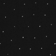
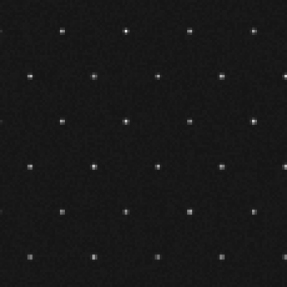
Experimental images from Refs. Samsonov2004, Feng2007 and RalphSPIE09 provide the benchmark for the images generated from simulations in this work. The raw images from the experiments reported in Ref. RalphSPIE09 compare very well to simulated images, as shown in Figures 2(a) and 2(b).

(a)  

(b)  

(c)  

(d)  

Figure 2: Zoomed versions of 2(a) a captured image from experiment, 2(b) a simulated image without camera defocussing, 2(c) a simulated single hexagonal lattice “cell” consisting of a central target particle surrounded by the six nearest neighbors. 2(d) a simulated image with simulated camera defocussing to increase pixel-resolution and reduce/remove pixel-locking errors. Images from experiments and simulations compare very well.

2.2 Nearest-Neighbor Approximation

Given the exponential suppression of the Yukawa force in Equation (2), it is reasonable to consider the relative effect of the Nearest-Neighbours (NNs) and the Next-Nearest-Neighbors (NNNs) on a “target” particle. For a crystal-like state where $r>\lambda_{\mathrm{D}}$, the exponential suppression factor suggests that the NNNs have relatively little influence on a target’s dynamics. We will now show that this is true by analyzing propagation of uncertainties. Uncertainties in the two-particle separation $r$ propagate into $F(r)$ as $\delta F(r)=\left|{(\partial F/\partial r)}\right|\delta r$, where $\partial F/\partial r$ calculated from Equation (2) is

$$\frac{\partial F}{\partial r}(\tilde{r})={\frac{k_{0}Q_{\mathrm{d}}^{2}}{\lambda_{\mathrm{D}}^{3}}e^{-\tilde{r}}\tilde{r}^{-3}\left({2+2\tilde{r}+\tilde{r}^{2}-\frac{1}{2}\tilde{r}^{3}}\right)}{\frac{k_{0}Q_{\mathrm{d}}^{2}}{\lambda_{\mathrm{D}}^{3}}e^{-\tilde{r}}\tilde{r}^{-3}\left({2+2\tilde{r}+\tilde{r}^{2}}\right)}$$ (7)

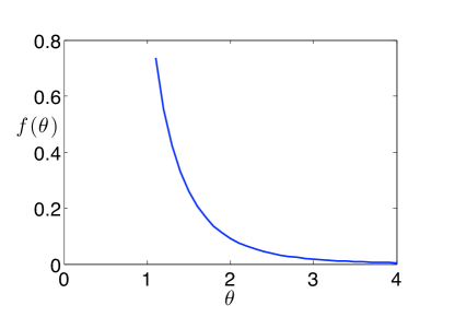
and the uncertainty in the particle separation will typically be $\delta r\leq\sqrt{2}\delta q$, where $\delta q$ is the largest measurement uncertainty in either dimension. That is, the average error in locating a particle’s center. In this work, $\delta q\sim 0.1$ pixels. Consider now the ratio between uncertainties in the two-particle forces due to NNs and NNNs: $\delta F(r_{\mathrm{NNN}})/\delta F(r_{\mathrm{NN}})$. If this ratio is sufficiently small, then we can safely omit the NNNs from the tracking algorithm. Defining $\theta\equiv r_{\mathrm{NNN}}/r_{\mathrm{NN}}>1$ and working in units of $\tilde{r}_{\mathrm{NN}}\equiv r_{\mathrm{NN}}/\lambda_{\mathrm{D}}$, we find that

$$f(\theta)\equiv\frac{\delta F(r_{\mathrm{NNN}})}{\delta F(r_{\mathrm{NN}})}={\frac{e^{-(\theta-1)}}{9}\left|{1-2\theta^{-1}-4\theta^{-2}-4\theta^{-3}}\right|}{\frac{e^{-(\theta-1)}}{5}\left({2\theta^{-3}+2\theta^{-2}+\theta^{-1}}\right)},$$ (8)

which is approaching insignificance ($f(\theta)<10\%$, say) for $\theta$ larger than approximately 2, as shown in Figure 3. Thus, for crystal-like states where $r_{\mathrm{NNN}}\approx 2r_{\mathrm{NN}}$, the tracking algorithm used need only consider the NNs and not the NNNs. This is a great reduction in complexity.

Figure 3: Plot of Equation (8) showing the effect of considering the next nearest neighbors (NNNs) in the tracking algorithm filter. The uncertainty in the predicted force on the tracked central particle is insignificant ($f(\theta)<10\%$, say) for $\theta>\sim 2$, which is always true for crystal-like structures of dusty plasmas where $r_{\mathrm{NNN}}\approx 2r_{\mathrm{NN}}$. If the NNNs move much closer than this, say $\theta<1.5$, then the influence of the NNNs may need to be considered in the tracking and state estimation algorithm.

2.3 Simulating a single hexagonal lattice cell

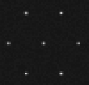
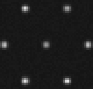
As shown in the preceding section, for a dusty plasma in a crystal-like phase, a target particle is only significantly affected by its NNs. Therefore, for the purposes of ascertaining (and quantifying) how the knowledge of surrounding particles can benefit the tracking process, this work focusses on a single cell of a hexagonal lattice, as seen in the experimental and theoretical work of Refs. Samsonov1999, Samsonov2004, Samsonov2000, Durniak2010, and Feng2007, for example. A small set of seven particles was simulated, representing a single cell of NNs surrounding a target particle in a hexagonal lattice as can be seen in Figures 2(c) and 2(d). The seven particles are initially positioned at an equidistant separation near potential minima (total potential: Yukawa plus confining potential) and interact via the Yukawa-type of potential (1) as described in Section 2. The shallow, parabolic, global confining potential is used to mimic the combined effect of many other surrounding particles and an experimental confining potential.[Durniak2010] These assumptions produce a reasonable model for a small subset of a larger two-dimensional dusty plasma in a crystal-like state.

3 STATE ESTIMATION AND TRACKING

3.1 Measurement: image-processing

Once images are obtained from a dusty plasma experiment (real or simulated), they are processed to determine the centroids (sub-pixel resolution location) of each particle. Herein, these centroids will be referred to as the particle measurements. The centroid location is achieved using one of a number of techniques described in Ref. Ivanov2007. The simplest of these is the Threshold Method (TM) where contiguous pixels above a certain threshold are considered to be a particle, with the pixel center-of-mass used for the centroid. The Moment Method (MM) works in a similar way to the TM, but calculates a center-of-mass weighted by the particle’s pixel-intensities. A third technique known as the Moment Method with Filter (MMF) involves applying a spatial bandpass filter (typically Gaussian) for smoothing and background subtraction prior to applying the MM to find the weighted center-of-mass. In typical order of increasing precision, these techniques are ranked TM, MM, MMF. There exist more sophisticated (and often more precise) measurement techniques, such as the Linear Quadratic Kernel Method[Ivanov2007], for which the increased computational expense cannot necessarily be justified for all applications, particularly if combining the measurements with a state-estimation algorithm that can improve the precision of the estimated positions for less computational expense.

Another option for improving the precision of dusty plasma particle measurements involves a hardware modification: defocussing the camera lens to obtain a “smeared” image to which the simpler (and faster) TM and MM methods can be applied. This approach (used here) helps to avoid errors due to “pixel-locking”[Feng2007, Ivanov2007] where certain sub-pixel locations are preferred due to low pixel-resolution caused when a particle only illuminates a small number of pixels. The particles in Figure 2(c) are of the order of 3 pixels across, whereas those in Figure 2(d) are approximately twice as large. The level of smearing can be modified to obtain a desired measurement precision, but it should be sufficiently moderate so as to not affect the measurement-track association process discussed in Section 3.2.

3.2 Measurement-track association

Each measurement must be either associated to a track, dismissed as a false alarm, or saved in memory as a possible new track. Along with the task of allowing for missed detections, this decision process is known as measurement-track association. In multi-target situations this can be a highly nontrivial task, especially when two or more targets are close to one another, for example. For simple situations where the targets remain spatially well-separated between subsequent measurements (Euclidean separation is greater than the measurement and prediction noise), a simple radar-like technique can be used to locate the measurement nearest to each track. This is the case for crystal-like dusty plasma structures close to equilibrium. This rather simple scenario provides a benchmark for measuring the performance of more sophisticated measurement-track association algorithms that are necessary for highly nonlinear dynamics such as Mach cones[Samsonov1999] and shock-waves[Samsonov2004].

3.3 The Extended Kalman Filter

The state estimation for the particle tracks uses a standard discrete-time Extended Kalman Filter (EKF)[BarShalom, JFRopaedia]. The state of each particle being tracked is represented by six variables – two positions $q_{\mathrm{x}}$ and $q_{\mathrm{y}}$, two velocities $v_{\mathrm{x}}$ and $v_{\mathrm{y}}$, and two accelerations $a_{\mathrm{x}}$ and $a_{\mathrm{y}}$ – at each time step $k=0,1,2\ldots$. The state is contained in a six-element vector: $\hat{x}(k)=(q_{\mathrm{x}},v_{\mathrm{x}},a_{\mathrm{x}},q_{\mathrm{y}},v_{\mathrm{y}},a_{\mathrm{y}})^{T}$ and the measurement for each particle is represented by a $2\times 6$ measurement matrix $H$:

$$H=\left(\begin{array}[]{cccccc}1&0&0&0&0&0\\ 0&0&0&1&0&0\end{array}\right)$$ (9)

so that the expected measurement for each track, given the previous measurements up to and including $k-1$, is given by

$$z(k|k-1)=H\cdot\hat{x}(k)=\left(\begin{array}[]{c}q_{\mathrm{x}}(k)\\ q_{\mathrm{y}}(k)\end{array}\right).$$ (10)

The expected and actual measurement ($z(k)$) at time step $k$ are combined to form the innovation (the difference between the expected positions and the measured positions) and added to the state vector as in the standard Kalman filter,

$$\hat{x}(k_{+})=\hat{x}(k)+K(k)\cdot(z(k)-z(k|k)),$$ (11)

where $\hat{x}(k_{+})$ indicates the updated state vector, the Kalman gain is given by $K(k)=S_{\hat{x}}(k)\cdot H^{T}\cdot(H\cdot S_{\hat{x}}(k)\cdot H^{T}+R(k))^{-1}$, $S_{\hat{x}}(k)$ is the estimated covariance matrix for the track states, and $R(k)$ is the expected covariance matrix for the measurement process being used.

After each time step, the particle state vector is predicted forward to the next time step using a discretization of the dynamical equations used in the simulation and given in Section 2

$${\hat{x}}(k+1)=f(\hat{x}(k_{+}))=\left(\begin{array}[]{c}q_{\mathrm{x}}(k_{+})+(\Delta t)v_{\mathrm{x}}(k_{+})+\frac{(\Delta t)^{2}F_{\mathrm{x}}(\hat{x}(k_{+}))}{2m}\\ v_{\mathrm{x}}(k_{+})+\frac{(\Delta t)F_{\mathrm{x}}(\hat{x}(k_{+}))}{m}\\ a_{\mathrm{x}}(k_{+})\\ q_{\mathrm{y}}(k_{+})+(\Delta t)v_{\mathrm{y}}(k_{+})+\frac{(\Delta t)^{2}F_{\mathrm{y}}(\hat{x}(k_{+}))}{2m}\\ v_{\mathrm{y}}(k_{+})+\frac{(\Delta t)F_{\mathrm{y}}(\hat{x}(k_{+}))}{m}\\ a_{\mathrm{y}}(k_{+})\\ \end{array}\right),$$ (12)

where $\Delta t$ is the time step. The corresponding equation for the predicted covariance is

$$S_{\hat{x}}(k+1)=f^{\prime}(k)\cdot S_{\hat{x}}(k_{+})\cdot f^{\prime}(k)^{T}+Q(k),$$ (13)

where $Q(k)$ is the process noise covariance, and

$$f^{\prime}(k)=\left.\frac{\partial f}{\partial\hat{x}}\right|_{\hat{x}=\hat{x}(k_{+})}.$$ (14)

This constitutes a piecewise linearization of the nonlinear particle dynamics represented by the simulation. This linear approximation should be accurate as long as the errors in the state estimates are small compared to the nonlinear nature of the underlying potential function. For the cases considered here, with the simulated dust particles in a crystal-like state, the relative movement of the particles around their equilibrium positions will be small enough for this approximation to hold. In more dynamic dusty plasmas, checks would be required to ensure that the estimated errors were not exceeding the ranges required for the perturbative expansion of the inter-particle forces about the current state estimates.

3.4 Process noise tuning

A tunable parameter for any EKF (or simple KF) is the process noise magnitude $\sigma_{\mathrm{Q}}$, which models the standard deviation for the highest-order time-derivative of position that is not included in the prediction model – in this case, the jerk (the time-derivative of acceleration). As these typical fluctuations are generally unknown a priori, $\sigma_{\mathrm{Q}}$ becomes a design parameter that needs to be optimized to help minimize modeling errors. This “process noise tuning” involves minimizing the average mean-square or root-mean-square (RMS) error as a function of $\sigma_{\mathrm{Q}}$. This is one example of where virtual experiments are beneficial because many experiments (perhaps hundreds or thousands) can be simulated to obtain good averages. For a typical simulation ensemble of size $N=1000$, $\sigma_{\mathrm{Q}}$ was varied over a finite range and the resulting average RMS error in the state estimate of the target particle’s position, $(q_{\mathrm{x}},q_{\mathrm{y}})$ was calculated as[BarShalom]

$$RMS(\sigma_{\mathrm{Q}},k)=\sqrt{\frac{1}{N}\sum_{i=1}^{N}\left[{(\Delta q_{\mathrm{x},i}(k))^{2}+(\Delta q_{\mathrm{y},i}(k))^{2}}\right]},$$ (15)

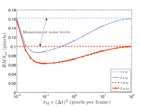
where $\Delta q_{\mathrm{x},i}(k)$ is the deviation of the estimated x-position from the true x-position at time $t(k)$ (and similarly for the y-direction). The long-time average of (15) provides a convenient measure of the filter’s performance as a function of $\sigma_{\mathrm{Q}}$. This is shown in Figure 4 (note the logarithmic horizontal axis), where data corresponding to TM measurements is blue and MM measurements is red (and bold). For increasingly large process noise magnitude, confidence in the prediction model decreases so that the measurements are “trusted” more by the filter and the RMS error in the estimated state asymptotically approaches the measurement noise level. An optimal process noise magnitude yields a minimum RMS error in the estimated state – note that the TM state estimate for a tuned filter performs better than the (non-optimized) MM measurement level, providing very encouraging support for a software-based approach to improving particle-locating precision, as opposed to what could be a laborious hardware optimization process in a real experiment in order to obtain comparable errors sizes. In any case, the state estimate outperforms the measurements for sufficiently large process noise, showing that it’s almost always beneficial to use any knowledge you have of the target particle dynamics to improve track precision via an EKF (the payoff decreases exponentially for less certain knowledge as the information processing costs outweigh the reduced improvement in precision).

The optimal values of process noise magnitude were $\sigma_{\mathrm{Q,TM}}(\Delta{t})^{2}=0.05$ pixels per frame and $\sigma_{\mathrm{Q,MM}}(\Delta{t})^{2}=0.1$ pixels per frame, where the sampling period used corresponds to imaging the virtual experiment at 200 frames per second: $\Delta{t}=0.005s$. The lower precision of TM measurements should result in a higher level of confidence (smaller $\sigma_{\mathrm{Q}}$) in the prediction model, and so the RMS errors in the state estimate are minimized for $\sigma_{\mathrm{Q,TM}}<\sigma_{\mathrm{Q,MM}}$.

Figure 4: For a single ensemble of 1000 virtual (simulated) experiments, multiple EKFs were run using a different process noise magnitude, expressed here in units of pixels per frame: $\sigma_{\mathrm{Q}}\times(\Delta{t})^{2}$. The optimal values (corresponding to fluctuations in particle positions of one-tenth and one-twentieth of a pixel per frame for MM and TM measurements, respectively) minimize the average RMS error (given here in pixels) over long times.

3.5 Filter consistency

For static parameter estimation, consistency of an estimator is defined as convergence of the estimate $\hat{x}$ to the true value $x$. For dynamic parameter estimation, estimator consistency is defined in terms of conditions on the first two moments of the estimate:[BarShalom]

$$E[x-\hat{x}] = 0,$$ (16a)

$$E[\left\{{x=\hat{x}}\right\}\left\{{x=\hat{x}}\right\}^{\prime}] = P.$$ (16b)

The first is satisfied by an unbiased estimator (zero-mean estimation error). The second condition is that of covariance matching between the MSE of the estimates (left-hand side) and the filter-calculated covariance (right-hand side). The two conditions in Equation (16) can be tested simultaneously using a $\chi$-squared test, as described in many undergraduate-level statistics texts – Ref. BarShalom describes it in the context of a Kalman filter. When the test statistics reside within an acceptance window, then the filter is determined to be consistent, which was the case in this work (although they are not presented here).

4 RESULTS AND DISCUSSION

(a)  Sample particle trajectory

(b)  Optimal RMS errors over time

Figure 5: Shown in 5(a) is a sample trajectory showing the true evolution of the target’s Y-position (thin black line), a spread of TM (blue $+$) and MM (red $\times$) measurements and the corresponding state estimates for the tuned process noise values given in Figure 4. Note the significantly larger deviation of the measurements compared to the estimates. Shown in 5(b) are the RMS errors in measured and estimated positions as a function of time, again for the tuned values of process noise. The sample period was $\Delta{t}=0.005$s (200 frames per second).

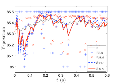
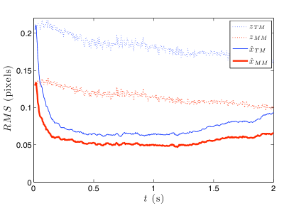
Figure 5(a) is a sample trajectory from the early stages of a single virtual experiment. The true Y-position of the central particle is shown as a thin black line, with the MM and TM measurements shown as crosses ($\times$) and plus signs ($+$), respectively. Shown are the state estimates generated by the EKF after processing each measurement and weighing it with the prediction model – the red line (MM) and blue dashed line (TM). Note the transient period before the filter “settles down” and tracks the true state quite well.

Figure 5(b) shows the RMS errors for the measurements (dotted lines) and estimated positions (solid lines) of the target particle when tracking only the target, but feeding the NN measurements into the prediction stage of the EKF. When tracking all 7 particles in the hexagonal “crystal” cell, the increased precision in the tracked NN positions did not significantly improve the target particle track. This is reasonable because the measurements were quite good, as shown earlier. For situations where the measurements are not so good (due to noisier images, for example), or the NN particles are moving faster, tracking the NNs (as opposed to just measuring them, which can represent a massive computational saving when tracking many particles) is expected to produce noticeably better results for the target track, albeit at a noticeably higher computational expense due to the increased number of states in the filter. For longer times than shown, the RMS error in the estimated position exhibits low-magnitude oscillations at a rate corresponding to the rate of oscillation of the interacting dust particles about the initial positions. This explains the apparent slight increase in the state estimate RMS errors at later times in Figure 5(b).

As shown in Section 3.4, the process noise magnitude $\sigma_{\mathrm{Q}}$ can be tuned to improve the EKF performance (minimize the errors in the estimated state). In the same way that the magnitude $\sigma_{\mathrm{Q}}$ represents confidence in the prediction model, the measurement noise magnitude $\sigma_{\mathrm{R}}$ represents confidence in the measurements. Figure 4 shows that the actual measurement errors were quite small: $\sigma_{\mathrm{R,TM}}\approx 0.16$ pixels, and $\sigma_{\mathrm{R,MM}}\approx 0.1$ pixels. In this work, no knowledge of the measurement precision was assumed and the so-called[hadziavdic2006] “worst-case scenario” of $\sigma_{\mathrm{R}}^{2}=0.1$ was used. Overestimating the measurement noise in this way is usually not as detrimental to the resulting performance of a Kalman filter as underestimating it, as shown for a simplified Kalman filter in Ref. hadziavdic2006. Therefore, it is expected that using a measurement noise size in the EKF that is closer to the true value would not significantly improve the EKF performance. Note that a similar tuning process can be performed for the measurement noise as was done for the process noise in Section 3.4.

(a)  True position

(b)  TM-measured position

(c)  MM-measured position

(d)  TM-based estimated position

(e)  MM-based estimated position

Figure 6: Sub-pixel maps for the central particle’s 6(a) true positions, 6(b) TM-measured positions, 6(c) MM-measured positions, 6(d) TM-based estimated positions, 6(e) MM-based estimated positions, across 1000 virtual experiments. Note the presence of pixel-locking in the TM measurements in 6(b) (and to a lesser extent in the MM measurements in 6(c)), and its subsequent removal by the EKF in 6(d).

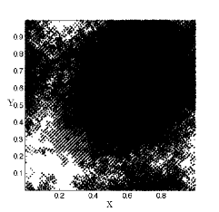
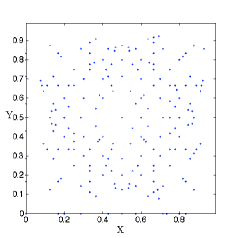
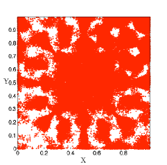
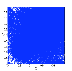
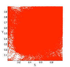
There are a few notable potential sources of error in tracking particles in dusty plasma experiments (both virtual and real). They can be categorized as measurement-based, model-based and numerical. The latter come in the form of round-off errors that can be minimized by using the Joseph form of the covariance update equation in the EKF.[BarShalom] Modeling errors, where an incorrect model is used for the system dynamics, can lead to incorrect predictions, and over- or under-confidence in predictions (versus measurements) due to sub-optimal process noise values – overcome here by the process-noise-tuning process. The most serious measurement-based errors for the rather unsophisticated techniques considered here (TM and MM) come in the form of “pixel-locking”,[Feng2007, Ivanov2007] resulting from insufficient pixel-resolution for the particles. This results in certain subpixel regions being preferred, as shown in Figure 6 where the measured subpixel locations (Figure 6(b) and 6(c)) of the target particle in 401 images from each of 1000 virtual experiments (401,000 data points) are plotted alongside the true (Figure 6(a)) and estimated (Figure 6(d) and 6(e)) subpixel locations. Pixel-locking was reduced for the MM measurements (see Figure 6(c)) in a fairly standard way – “smearing” the particles slightly by defocussing the virtual camera. Remarkably, although this technique was completely unsuccessful for the TM measurements (see Figure 6(b)), the filter almost completely removed the pixel-locking effect as shown in the subpixel map for the TM-based estimates in Figure 6(d). These maps were representative of all the particles. They show that strong pixel-locking occurred for the TM measurements (and to a lesser extent for the MM measurements), but was removed after processing these measurements through the filter.

5 CONCLUSION

An extended Kalman filter (EKF) algorithm has been designed and implemented for tracking interacting dusty plasma particles. The algorithm was tested in virtual experiments (simulations) which allowed for quantification of performance aspects such as the precision of locating particle positions. Attention was paid to generating images that closely resemble real experiments. The algorithm was tested for a crystal-like phase of the dusty plasma. This simple scenario provides a benchmark for measuring the performance of more sophisticated algorithms that will be necessary for treating more complex dynamics. An analytical result showed the validity of an approximation to only nearest-neighbor interactions for this situation. Starting with relatively imprecise measurements of particle positions using the threshold and moment methods, it was shown that the filter algorithm improved the precision, as well as removing or significantly reducing errors due to “pixel-locking”. The RMS values of position errors exceeded $0.1$ pixels for the measurements, which were improved by the filter to approximately $0.06$ pixels – approaching the precision obtained in Ref. Ivanov2007 ($\approx 0.03$ pixels) where a much more sophisticated and time-consuming measurement technique was used (local quadratic kernel method). This suggests that when such “cheap” measurements are used in conjunction with an EKF, they may be sufficient for obtaining excellent sub-pixel precision for particle positions – a task that was previously achieved through hardware modifications and/or the aforementioned sophisticated measurement (image-processing) techniques. This particular result bodes well for eventually applying such a particle-tracking filter in real-time, perhaps as part of a feedback loop.

It is expected that the algorithm’s will perform quite wellperformance in experimental situations will be comparable to the results presented here, but performance will degrade the further a dusty plasma deviates from a crystal-like state. Future work includes applying the algorithm to experimental images, extending the algorithm to cope with highly nonlinear dynamics such as shock-waves and Mach cones, and considering more advanced state estimation and measurement-track association techniques. The present results will provide a useful performance benchmark for future work.