Quasispecies dynamics with network constraints

Abstract

A quasispecies is a set of interrelated genotypes that have reached a situation of equilibrium while evolving according to the usual Darwinian principles of selection and mutation. Quasispecies studies invariably assume that it is possible for any genotype to mutate into any other, but recent finds indicate that this assumption is not necessarily true. Here we revisit the traditional quasispecies theory by adopting a network structure to constrain the occurrence of mutations. Such structure is governed by a random-graph model, whose single parameter (a probability $p$) controls both the graph’s density and the dynamics of mutation. We contribute two further modifications to the theory, one to account for the fact that different loci in a genotype may be differently susceptible to the occurrence of mutations, the other to allow for a more plausible description of the transition from adaptation to degeneracy of the quasispecies as $p$ is increased. We give analytical and simulation results for the usual case of binary genotypes, assuming the fitness landscape in which a genotype’s fitness decays exponentially with its Hamming distance to the wild type. These results support the theory’s assertions regarding the adaptation of the quasispecies to the fitness landscape and also its possible demise as a function of $p$.

I Introduction

The concept of a quasispecies was introduced by Eigen and Schuster Eigen (1971); Eigen and Schuster (1977) to describe the equilibrium state of a population of genotypes whose members mutate frequently into one another while replicating without recombination (i.e., asexually). At first the theory targeted the dynamics of complex, prebiotic molecules and aimed to explain the phenomena of self-organization and adaptability that led to the appearance of life. Today, however, the quasispecies theory is thought to be much more widely applicable, as to the dynamics of RNA viruses and in cancer research Más et al. (2010), in fact providing interesting insight into the dynamics of any population of genotypes, including those that replicate with recombination and mutate relatively infrequently Nowak and May (2000).

The theory combines the evolutionary principles of selection and mutation to describe the dynamics of a population of genotypes, and in this sense constitutes the leading manifestation of the Darwinian principles at the molecular level. Its central tenet is that, although each individual genotype can be ascribed a fitness that is a function of its replicative capacity, the actual fitness effects (ranging, e.g., from strongly deleterious to highly adaptive Orr (2003); Sanjuán et al. (2004); Eyre-Walker and Keightley (2007)) are a property of the population rather than of the genotype Schuster and Swetina (1988). As we observe the dynamics of the population relative to the so-called fitness landscape (i.e., the fitnesses of all possible genotypes), selection operates on the entire population and can guide it toward the landscape’s peaks. In other words, even though the process of mutation remains essentially stochastic, the population can in fact influence it because the fittest genotypes will replicate more and lead the population to adapt to the fitness landscape.

In the particular case of RNA viruses, and notwithstanding some degree of controversy over how applicable the quasispecies theory is to their dynamics (cf., e.g., Domingo (2002); Holmes and Moya (2002) and more recently Holmes (2010); Más et al. (2010)), the array of implications to the understanding of viral diseases is notable. For example, the theory suggests that the fitness effects of a virus population are determined more by how free its various genotypes are to mutate than by how capable they are to replicate. Another implication seems to be that, paradoxically, increasing the genotypes’ error rates during replication may render the virus less pathogenic Domingo (2009); Lauring and Andino (2010).

The centerpiece of the quasispecies theory is the so-called quasispecies equation, which for each possible genotype gives the rate at which the genotype’s relative abundance varies with time in terms of all genotypes’ abundances, their fitnesses, and the rates at which genotypes mutate into one another. We refer the reader to Biebricher and Eigen (2006); Nowak (2006), and references therein, for a summary of the customary assumptions and known developments. Normally a genotype is represented as a length-$L$ string of $0$’s and $1$’s, so the number of genotypes in the population is $2^{L}$. Every genotype can mutate into every other, so essentially there is no structure constraining the occurrence of mutations. Moreover, in general one assumes that mutations can be modeled as occurring independently at each of a genotype’s loci with the same probability $u$ for each locus (a notable exception here is the study in Saakian and Hu (2006), where loci having different mutation rates are allowed, as are mutations of two or three adjacent loci as a group, in recognition of the plausibility of such events Averof et al. (2000); Deng and Fu (2000); Nachman and Crowell (2000)).

In addition to the quasispecies itself, which is characterized by the genotypes’ relative abundances at equilibrium, another important observable in the theory is the so-called error threshold, which refers to how variations in the point mutation rate $u$ determine the population’s average fitness at equilibrium. The customary approach to determine this threshold is to concentrate on the relative abundance of the fittest genotype, normally called the wild (or master) type, and study how its eventual survival depends on $u$. Invariably such studies have assumed that no genotype can mutate into the wild type and solved the resulting, simplified version of the quasispecies equation for the minimum value of $u$ that ensures that the wild type survives. This threshold value is a function of the wild type’s fitness and of the length $L$ Biebricher and Eigen (2006); Nowak (2006); Saakian and Hu (2006).

Here we revisit the quasispecies theory by seeking to attenuate what we perceive to be three main sources of biological implausibility. The first one is related to the total lack of structure constraining the possible mutations inside the population. Recent finds indicate, to the contrary, that for some organisms not every combination of loci can be involved in a single mutation out of a specific genotype de Visser et al. (2009). The second one has to do with the nearly ubiquitous assumption that genotypes are equally likely to undergo a mutation at any locus. In this case, too, there is evidence in support of locus-dependent mutation rates Deng and Fu (2000) even though mutations do seem to occur simultaneously at different, not necessarily contiguous, loci Whelan and Goldman (2004).

We tackle these first two issues by adopting a susceptibility model to differentiate one locus from another as far as the occurrence of mutations at those loci is concerned. The susceptibility of a specific locus $\ell$ is any positive number $s_{\ell}$ that gets larger as genotypes become more susceptible to the occurrence of a mutation at locus $\ell$. Given two genotypes $i$ and $j$ that differ at locus $\ell$ and a probability parameter $p$, we use $p^{1/s_{\ell}}$ both to create a random-graph model to give structure to the evolving population in terms of whether $i$ and $j$ can mutate into each other and to govern the dynamics of mutation if they can. Additionally, note that by adopting a random-graph model into the quasispecies theory we are also providing the theory with a perspective that connects it with the decade-long effort to understand the so-called complex networks and their applications Bornholdt and Schuster (2003); Newman et al. (2006); Bollobás et al. (2009).

Our third perceived source of implausibility comes from the assumptions that underlie the common method to determine the error threshold. Such assumptions are too stringent (no genotype mutates into the wild type) and result in a strict threshold separating the survival of the wild type in the quasispecies from its catastrophic demise. Rather, as suggested by the study in Wilke and Ronnewinkel (2001) and the review in Lauring and Andino (2010), we believe it might be more plausible if the two regimes were separated by a wider interval of the control parameter ($p$, in our case), over which the transition could occur more smoothly. In order to avoid the same stringent assumptions that have dominated such studies so far, we start by assuming instead that a genotype’s relative abundance in the quasispecies depends on its fitness as a power law. The accuracy of this assumption depends on the susceptibilities of the various loci, but in the cases we investigate it allows the average fitness of the quasispecies to be expressed analytically and the transition between degeneracy and survival to occur smoothly.

We proceed in the following manner, assuming that genotypes are binary (as usual) and also that a genotype’s fitness decays exponentially with its Hamming distance to the wild type. First we introduce our model in Sec. II, where we rewrite the quasispecies equation for the case of network-constrained mutations and, for two distinct susceptibility scenarios, solve it approximately under the assumption that a genotype’s relative abundance and fitness are related by a power law. Then we give computational results in Sec. III and also discuss the conditions for our analytical expressions to be good approximations to the simulation data. We conclude in Sec. IV.

II Model

We consider binary genotypes of length $L$, that is, length-$L$ sequences of $0$’s and $1$’s. There are thus $n=2^{L}$ different genotypes, numbered $1,2,\ldots,n$. We assume that genotype $1$ comprises only $0$’s. The fitness of genotype $i$ reflects its replication rate and here is given by $f_{i}=2^{-d_{i}}$, where $d_{i}$ is the number of $1$’s in the genotype. That is, a genotype’s fitness decays exponentially with its Hamming distance to genotype $1$ (which is then the fittest one, with $f_{1}=1$, or wild type). While this choice seems reasonable, it is by no means the only possibility and many other alternatives might be considered. We note, however, that adopting an exponential function has allowed many of the analytical calculations that we present in this section to be performed.

We assume that the $n$ genotypes are the nodes of a directed graph $D$ with self-loops at all nodes. The set of in-neighbors of node $i$ in $D$ is denoted by $I_{i}$ and its set of out-neighbors by $O_{i}$. It holds that both $i\in I_{i}$ and $i\in O_{i}$. The existence of an edge directed from node $i$ to node $j\neq i$ means that it is possible for genotype $i$ to mutate into genotype $j$ during replication. This happens with probability $q_{ij}$. Letting $q_{ii}$ be the probability that genotype $i$ remains unchanged during replication leads to $\sum_{j\in O_{i}}q_{ij}=1$.

Let $X_{i}$ denote the abundance of genotype $i$ at any given time, and similarly let $x_{i}=X_{i}/\sum_{k=1}^{n}X_{k}$ be its relative abundance. The time derivative of $X_{i}$ depends on the abundance of all genotypes in $I_{i}$ (i.e., $i$ itself and those that can mutate into $i$ during replication) in such a way that

$$\dot{X}_{i}=\sum_{j\in I_{i}}f_{j}q_{ji}X_{j}.$$ (1)

Rewriting for $x_{i}$ yields

$$\dot{x}_{i}=\sum_{j\in I_{i}}f_{j}q_{ji}x_{j}-\phi x_{i},$$ (2)

where $\phi=\sum_{k=1}^{n}f_{k}x_{k}$ is the average fitness of all $n$ genotypes. Equation (2) is the well-known quasispecies equation, now written for graph $D$.

In our model, both the structure of graph $D$ and the dynamics of mutation depend on how susceptible each of the $L$ loci in a genotype is to undergo a mutation. For $\ell=1,2,\ldots,L$, we let $s_{\ell}$ be a positive number that grows with the susceptibility that a genotype undergoes a mutation at locus $\ell$, the same for all genotypes. Thus, an edge exists in graph $D$ directed from genotype $i$ to genotype $j$ with probability $p_{ij}$ such that

$$p_{ij}=p^{\sum_{\ell=1}^{L}h_{\ell}/s_{\ell}},$$ (3)

where $p$ is a probability parameter and $h_{\ell}=1$ if and only if the two genotypes differ at locus $\ell$ ($h_{\ell}=0$, otherwise). Note that this definition of $p_{ij}$ is consistent with the mandatory existence of self-loops at all nodes of $D$, since for $j=i$ we have $h_{\ell}=0$ for all $\ell$ and thus $p_{ii}=1$. If the edge from $i$ to $j$ does exist, the probability $q_{ij}$ that $i$ mutates into $j$ (or remains unchanged, if $j=i$) is proportional to $p_{ij}$, i.e., $q_{ij}=p_{ij}/Z_{i}$, where $Z_{i}=\sum_{k\in O_{i}}p_{ik}$ is a normalizing constant for genotype $i$.

Henceforth we work on the hypothesis that, at equilibrium, $x_{i}$ depends on the fitness $f_{i}$ as a power law for every genotype $i$. That is, we assume that $x_{i}=bf_{i}^{a}$ for suitable $a>0$ when $\dot{x_{i}}=0$. Such functional dependency turns up in some of the cases we study (cf. Sec. III) and, furthermore, facilitates some of the analytical calculations that we carry out in this section. It immediately follows that the equilibrium value of the average fitness is $\phi=b\sum_{h=0}^{L}{L\choose h}2^{-(a+1)h}$, yielding

$$\phi=b\left[1+2^{-(a+1)}\right]^{L}.$$ (4)

Moreover, from the constraint $\sum_{i=1}^{n}x_{i}=1$ we obtain $b\sum_{h=0}^{L}{L\choose h}2^{-ah}=1$, whence

$$b=(1+2^{-a})^{-L}.$$ (5)

We estimate the value of $a$ by resorting to a mean-field version of Eq. (2), that is, one in which the expected contribution of every genotype $j$ to $\dot{x}_{i}$ (not only those in $I_{i}$) is taken into account and occurs according to the expected value of the mutation probability $q_{ji}$ of genotype $j$ into genotype $i$. By definition, mutation in this case occurs with probability proportional to $p_{ji}$, provided graph $D$ contains an edge directed from $j$ to $i$. The latter happens with probability $p_{ji}$ as well, so the expected value of $q_{ji}$ is $p_{ji}^{2}/\sum_{k=1}^{n}p_{jk}^{2}$. Equation (2) then becomes

$$\dot{x}_{i}=\sum_{j=1}^{n}\frac{f_{j}p_{ji}^{2}x_{j}}{\sum_{k=1}^{n}p_{jk}^{2}}-\phi x_{i}.$$ (6)

Our estimate of $a$ comes from considering the wild type at equilibrium, that is, from imposing $\dot{x}_{1}=0$ in Eq. (6) and solving the resulting equation,

$$\sum_{j=1}^{n}\frac{p_{j1}^{2}2^{-(a+1)d_{j}}}{\sum_{k=1}^{n}p_{jk}^{2}}-\left[\frac{1+2^{-(a+1)}}{1+2^{-a}}\right]^{L}=0.$$ (7)

We study two susceptibility scenarios. The first one, henceforth referred to as the uniform case, sets $s_{\ell}=1$ for every locus $\ell$. In this case, it follows that $\sum_{\ell=1}^{L}h_{\ell}/s_{\ell}$ in Eq. (3) is the Hamming distance between genotypes $i$ and $j$, here denoted by $H_{ij}$, and therefore $p_{ij}=p^{H_{ij}}$. The summation on $k$ appearing in Eq. (7) becomes

$$\sum_{k=1}^{n}p_{jk}^{2}=\sum_{h=0}^{L}{L\choose h}p^{2h}=(1+p^{2})^{L}$$ (8)

for any $j$ and the summation on $j$, since $p_{j1}=p^{d_{j}}$, can be similarly written as a sum on the possible values $h$ of the Hamming distance $d_{j}$ to the wild type:

$$\sum_{j=1}^{n}p_{j1}^{2}2^{-(a+1)d_{j}}=\sum_{h=0}^{L}{L\choose h}p^{2h}2^{-(a+1)h}.$$ (9)

This yields

$$\frac{1+p^{2}2^{-(a+1)}}{1+p^{2}}=\frac{1+2^{-(a+1)}}{1+2^{-a}},$$ (10)

whence

$$2^{a}=\frac{1+\sqrt{1+8p^{4}}}{4p^{2}},$$ (11)

so in the uniform case the value of the power-law exponent $a$ does not depend on $L$. For sufficiently small $p$, we can write $2^{a}\approx 1/2p^{2}$, which by Eqs. (4) and (5) allows the equilibrium value of $\phi$, in the uniform case, to be approximated by

$$\phi=\left(\frac{1+p^{2}}{1+2p^{2}}\right)^{L}\approx e^{-Lp^{2}}$$ (12)

for large $L$.

In the second susceptibility scenario, which we henceforth refer to as the inverse-decay case, we have $s_{\ell}=1/\ell$ for locus $\ell$. While this specific form for the dependency of $s_{\ell}$ on $\ell$ is totally arbitrary and seems to carry no special biological meaning, it has been our choice because it is simple and has proven amenable to a certain degree of analytical manipulation. It this case it follows that $\sum_{\ell=1}^{L}h_{\ell}/s_{\ell}=\sum_{\ell=1}^{L}h_{\ell}\ell$ in Eq. (3), which is the sum of every $\ell$ such that genotypes $i$ and $j$ differ at locus $\ell$. Denoting this sum by $T_{ij}$ yields $p_{ij}=p^{T_{ij}}$. Now the summation on $k$ appearing in Eq. (7) becomes

$$\sum_{k=1}^{n}p_{jk}^{2}=\sum_{s=0}^{L(L+1)/2}T(L,s)p^{2s}=\prod_{\ell=1}^{L}(1+p^{2\ell})$$ (13)

for any $j$, where $T(L,s)$ is the number of genotypes that differ from genotype $j$ in loci that sum up to $s$ . The summation on $j$, in turn, depends on first recognizing that the collective contribution to it from all $L\choose h$ nodes $j$ whose Hamming distance to the wild type is $d_{j}=h$ for fixed $h$ is proportional to

$$2^{-(a+1)h}\sum_{s=0}^{L(L+1)/2}T_{h}(L,s)p^{2s},$$ (14)

where $T_{h}(L,s)$ is the number of genotypes whose $h$ $1$’s are found at loci that sum up to $s$ . While the summation in this expression cannot be written in a simpler form, it can be shown that the average value of $s$ over the $L\choose h$ genotypes involved is $(L+1)h/2$ . We then approximate that summation by ${L\choose h}p^{(L+1)h}$, so once again the summation on $j$ in Eq. (7) can be written as a sum on the possible values $h$ of the Hamming distance $d_{j}$ between the wild type and genotype $j$:

$$\sum_{j=1}^{n}p_{j1}^{2}2^{-(a+1)d_{j}}\approx\sum_{h=0}^{L}{L\choose h}p^{(L+1)h}2^{-(a+1)h}.$$ (15)

For $f(L,p)$ such that $\prod_{\ell=1}^{L}(1+p^{2\ell})=[1+f(L,p)]^{L}$, this leads to

$$\frac{1+p^{L+1}2^{-(a+1)}}{1+f(L,p)}\approx\frac{1+2^{-(a+1)}}{1+2^{-a}},$$ (16)

and finally to

$$2^{a} \approx \frac{1+p^{L+1}-f(L,p)}{4f(L,p)}+$$ (17)

$$\frac{\sqrt{[1+p^{L+1}-f(L,p)]^{2}+8f(L,p)p^{L+1}}}{4f(L,p)}.$$

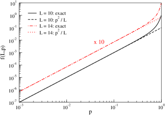
For $p<0.2$, we have found empirically that $f(L,p)\approx p^{2}/L$ (Fig. 1), whence $2^{a}\approx(1-p^{2}/L)/(2p^{2}/L)$ for large $L$. It then follows from Eqs. (4) and (5) that, in the inverse-decay case, the equilibrium value of $\phi$ can be approximated by

$$\phi=\left(\frac{1}{1+p^{2}/L}\right)^{L}\approx e^{-p^{2}}.$$ (18)

Figure 1: (Color online) Approximation of $f(L,p)$ by $p^{2}/L$ in the inverse-decay case.

III Results

For fixed values of the length $L$ and the probability parameter $p$, our results are based on generating $10^{4}$ independent instances of graph $D$ and solving Eq. (2) numerically for each instance. This is achieved by letting $x_{i}=1/n$ initially for $i=1,2,\ldots,n$ (i.e., the initial population is uniform on all genotypes) and time-stepping the corresponding equations until $\sum_{i=1}^{n}|\dot{x}_{i}|<10^{-8}$. Because this entails substantial computational effort, we limit ourselves to $L=10$ and $L=14$ (i.e., $n=1\,024$ and $n=16\,384$ distinct genotypes, respectively).

The resulting relative abundances of the quasispecies are given in Fig. 2 as a function of the genotypes’ fitnesses. By definition there are in general several different genotypes of the same fitness, so in the figure we give the average relative abundance of all such genotypes. In the uniform case, these results reveal an average behavior of same-fitness genotypes that is in excellent agreement with the power-law assumption we made. Moreover, as indicated by Eq. (11), the power-law exponent $a$ does not depend on $L$, being a function of $p$ exclusively. In the inverse-decay case, on the other hand, the power-law assumption is reasonable only for the highest fitness values. At these values, it is worth noting that the power-law exponent $a$ as given by Eq. (17) behaves reasonably with respect to the data despite the approximation of the summation in Eq. (14) by ${L\choose h}p^{(L+1)h}$. The reason for this is that, once these expressions get multiplied by $2^{-(a+1)h}$ and summed up on $h$, the results are dominated by the lowest $h$ values, hence the highest fitnesses, and these are precisely the values at which the approximation works best [in fact, both the summation in Eq. (14) and its approximation yield $1$ for $h=0$, since $T_{0}(L,s)=1$ if $s=0$ and $T_{0}(L,s)=0$ otherwise].

Figure 2: (Color online) Relative abundances at equilibrium. For each fitness $2^{-h}$, where $h$ is one of the possible values of the Hamming distance to the wild type, data are averages over all $L\choose h$ genotypes that have that fitness and $10^{4}$ independent instances of graph $D$. Lines refer to the power law of exponent $a$ as given by Eq. (11) in the uniform case or Eq. (17) in the inverse-decay case.

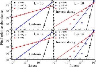
Figure 2 also reveals how the dominance of the wild type in the population behaves as $p$ is increased and mutations into ever more different genotypes begin to be both allowed by the structure of $D$ and made more frequent during the dynamics. A clearer view into this is afforded by Fig. 3, where we show the relative abundance of the wild type in the quasispecies as a function of $p$. Clearly, in both the uniform and the inverse-decay cases there exist values of $p$ beyond which the wild type gets diluted into the population just as all other genotypes do. This happens at higher values in the inverse-decay case, since the $1/\ell$ susceptibility for locus $\ell$ tends to discourage mutations at this locus for all but relatively small values of $\ell$ despite increases in $p$.

Figure 3: (Color online) Relative abundance of the wild type at equilibrium. Data are averages over $10^{4}$ independent instances of graph $D$. Lines refer to $x_{1}=bf_{1}^{a}=b$ for $a$ as given by Eq. (11) in the uniform case or Eq. (17) in the inverse-decay case.

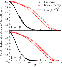
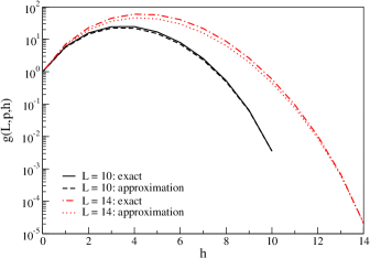
Figure 3 also illustrates how well the power-law exponent $a$ in Eq. (11) or (17) does when we focus on the wild type across the entire range for $p$. While the agreement with the data is once again very good in the uniform case, in the inverse-decay case this holds only for roughly $p<0.2$ or $p>0.9$. As above, explaining this requires that we revisit the approximation of the summation in Eq. (14) by ${L\choose h}p^{(L+1)h}$. Specifically, as we sum the product of either quantity by $2^{-(a+1)h}$ on $h$, sufficiently small values of $p$ render the differences caused by the approximation irrelevant. Similarly, for sufficiently large values of $p$ the approximation is good across a wide range of $h$ values, as shown in Fig. 4.

Figure 4: (Color online) Comparison between the summation in Eq. (14), here referred to as $g(L,p,h)$, and ${L\choose h}p^{(L+1)h}$ for $p=0.95$.

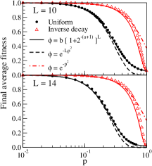
A better glimpse into wild-type survival comes from considering the average fitness $\phi$ of the quasispecies. This is depicted in Fig. 5, which clearly indicates that the transition from survival to degeneracy of the wild type occurs gradually, within roughly one order of magnitude of the parameter $p$ as it is increased. In the figure we also display our analytical predictions for $\phi$ at equilibrium. These are given, through Eqs. (4) and (5), as functions of the power-law exponent $a$ in Eqs. (11) and (17). The same observations on accuracy given above continue to apply. Figure 5 also contains the simpler approximation of $\phi$ at equilibrium given by the Gaussians in Eqs. (12) and (18), respectively for the uniform case and the inverse-decay case. As expected, these approximations work very well for small values of $p$. The one for the uniform case tends to improve as $L$ is increased.

Figure 5: (Color online) Average fitness at equilibrium. Data are averages over $10^{4}$ independent instances of graph $D$. Lines refer to Eqs. (4) and (5) with $a$ as given by Eq. (11) in the uniform case or Eq. (17) in the inverse-decay case, or to the Gaussian of Eq. (12) in the uniform case or Eq. (18) in the inverse-decay case.

IV Conclusions

We have revisited the quasispecies theory and examined what we believe to be drawbacks in its customary modeling assumptions. These are the absence of an underlying structure separating the mutations that can occur from those that cannot; the lack of a general framework within which a genotype’s loci can be sorted into different susceptibilities to undergo mutations; and finally, a methodology to explain the degeneracy of the wild type, when mutations are excessively too frequent, that implies a brusque transition from the regime in which it survives. Our approach to tackle these issues has been, respectively, to model the mutational interactions among genotypes as a random graph; to adopt real-valued susceptibilities that influence both the graph’s structure and the dynamics of the population; and to postulate a specific functional dependency of a genotype’s relative abundance on its fitness at equilibrium. The resulting model has a probability, $p$, as its single parameter. Increasing $p$ makes the graph denser and allows more mutations as the population evolves toward the quasispecies.

It is important to note that our model does not merely generalize the common approach of assuming that graph $D$ has an edge directed from any genotype to any other and that any locus in a genotype is equally susceptible to undergo a mutation at the same point rate $u$. Even though in the two models it is sometimes possible to write the mutation probability $q_{ij}$ of genotype $i$ into genotype $j$ as very similar products over all $L$ loci [in the customary approach we have $q_{ij}=u^{H_{ij}}(1-u)^{L-H_{ij}}$; in our model, assuming for example the uniform case, we have $q_{ij}=(p/Z_{i}^{1/L})^{H_{ij}}(1/Z_{i}^{1/L})^{L-H_{ij}}$], the similarity between them can be carried no further. In fact, setting $p=1$ in our model to ensure that $D$ is always fully connected yields $q_{ij}=1/n=0.5^{L}$ regardless of $i$ or $j$, which does not conform with the usual approach unless $u=0.5$. The bottom line is that substantial further studies are needed to determine whether characteristic values of $p$ exist for as many organisms as possible, much as has been done for the rate $u$ (cf., e.g., Nowak (2006)).

Our results were given for the nontrivial fitness landscape in which a genotype’s fitness decays exponentially with its Hamming distance to the wild type. They have also been based on two specific susceptibility scenarios and a power-law relationship between a genotype’s relative abundance in the quasispecies and its fitness. While the latter is widely accurate only for one of the susceptibility scenarios (the uniform case), overall our modeling choices have led to useful analytical predictions of both the several genotypes’ participation in the quasispecies and the wild type’s transition from survival to degeneracy as $p$ increases.

As with other variations of the quasispecies theory, the modifications we have introduced all corroborate the theory’s central idea, viz. that selection and mutation act on the entire ensemble of genotypes. They also corroborate the crucial role of the error-related parameter ($p$, in our case) in separating two distinct regimes, one in which the quasispecies adapts to the fitness landscape, the other in which it becomes degenerate. It remains to be seen whether the same will continue to hold as alternative fitness landscapes and variations of the remaining assumptions are studied.