University of Alberta, Edmonton, Alberta, Canada
Multi-timescale Nexting
in a Reinforcement Learning Robot
Abstract
The term “nexting” has been used by psychologists to refer to the propensity of people and many other animals to continually predict what will happen next in an immediate, local, and personal sense. The ability to “next” constitutes a basic kind of awareness and knowledge of one’s environment. In this paper we present results with a robot that learns to next in real time, predicting thousands of features of the world’s state, including all sensory inputs, at timescales from 0.1 to 8 seconds. This was achieved by treating each state feature as a reward-like target and applying temporal-difference methods to learn a corresponding value function with a discount rate corresponding to the timescale. We show that two thousand predictions, each dependent on six thousand state features, can be learned and updated online at better than 10Hz on a laptop computer, using the standard TD() algorithm with linear function approximation. We show that this approach is efficient enough to be practical, with most of the learning complete within 30 minutes. We also show that a single tile-coded feature representation suffices to accurately predict many different signals at a significant range of timescales. Finally, we show that the accuracy of our learned predictions compares favorably with the optimal off-line solution.
1 Multi-timescale Nexting
Psychologists have noted that people and other animals seem to continually make large numbers of short-term predictions about their sensory input (e.g., see Gilbert 2006, Brogden 1939, Pezzulo 2008, Carlsson et al. 2000). When we hear a melody we predict what the next note will be or when the next downbeat will occur, and are surprised and interested (or annoyed) when our predictions are disconfirmed (Huron 2006, Levitin 2006). When we see a bird in flight, hear our own footsteps, or handle an object, we continually make and confirm multiple predictions about our sensory input. When we ride a bike, ski, or rollerblade, we have finely tuned moment-by-moment predictions of whether we will fall, and of how our trajectory will change in a turn. In all these examples, we continually predict what will happen to us next. Making predictions of this simple, personal, short-term kind has been called nexting (Gilbert, 2006).
Nexting predictions are specific to one individual and to their personal, immediate sensory signals or state variables. A special name for these predictions seems appropriate because they are unlike predictions of the stock market, of political events, or of fashion trends. Predictions of such public events seem to involve more cognition and deliberation, and are fewer in number. In nexting we envision that one individual may be continually making massive numbers of small predictions in parallel. Moreover, nexting predictions seem to be made simultaneously at multiple time scales. When we read, for example, it seems likely that we next at the letter, word, and sentence levels, each involving substantially different time scales.
The ability to predict and anticipate has often been proposed as a key part of intelligence (e.g., see Tolman 1951, Hawkins & Blakeslee 2004, Butz et al. 2003, Wolpert et al. 1995, Clark in press). Nexting can be seen as the most basic kind of prediction, preceding and possibly underlying all the others. That people and a wide variety of animals learn and make simple predictions at a range of short time scales in conditioning experiments was established so long ago that it is known as classical conditioning (Pavlov 1927). Predictions of upcoming shock to a paw may reveal themselves in limb-retraction attempts a fraction of a second before the shock, and as increases in heart rate 30 seconds prior. In other experiments, for example those known as sensory preconditioning (Brogden 1939, Rescorla 1980), it has been clearly shown that animals learn predictive relationships between stimuli even when none of them are inherently good or bad (like food and shock) or connected to an innate response. In this case the predictions are made, but not expressed in behaviour until some later experimental manipulation connects them to a response. Animals seem to just be wired to learn the many predictive relationships in their world.
To be able to next is to have a basic kind of knowledge about how the world works in interaction with one’s body. It is to have a limited form of forward model of the world’s dynamics. To be able to learn to next—to notice any disconfirmed predictions and continually adjust your nexting—is to be aware of one’s world in a significant way. Thus, to build a robot that can do both of these things is a natural goal for artificial intelligence. Prior attempts to achieve artificial nexting can be grouped in two approaches.
The first approach is to build a myopic forward model of the world’s dynamics, either in terms of differential equations or state-transition probabilities (e.g., Wolpert et al. 1995, Grush 2004, Sutton 1990). In this approach a small number of carefully chosen predictions are made of selected state variables with a public meaning. The model is myopic in that the predictions are only short term, either infinitesimally short in the case of differential equations, or maximally short in the case of the one-step predictions of Markov models. In these ways, this approach has ended up in practice being very different from nexting.
The second approach, which we follow here, is to use temporal-difference (TD) methods to learn long-term predictions directly. The prior work pursuing this approach has almost all been in simulation, and has used table-lookup representations and a small number of predictions (e.g., Sutton 1995, Kaelbling 1993, Singh 1992, Sutton, Precup & Singh 1999, Dayan and Hinton 1993). Sutton et al. (2011) showed real-time learning of TD predictions on a robot, but did not demonstrate the ability to learn many predictions in real time or with a single feature representation.
2 Nexting as Multiple Value Functions
We take a reinforcement-learning approach to achieving nexting. In reinforcement learning it is commonplace to learn long-term predictions of reward, called value functions, and to learn these using temporal-difference (TD) methods such as TD() (Sutton 1988). However, TD() has also been used as a model of classical conditioning, where the predictions are shorter term and where more than one signal might be viewed as a reward (Sutton & Barto, 1990). Our approach to nexting can be seen as taking this latter approach to the extreme of predicting massive numbers of target signals of all kinds at multiple time scales.
We use a notation for our multiple predictions that mirrors—or rather multiplies—that used for conventional value functions. Time is taken to be discrete, , with each time step corresponding to approximately 0.1 seconds of real time. Our th prediction at time , denoted , is meant to anticipate the future values of the th prediction’s target signal, , over a designated time scale given by the discount-rate parameter . In our experiments, the target signal was either a raw sensory signal or else a component of a state-feature vector (that we will introduce shortly), and the discount-rate parameter was one of four fixed values. The goal of learning is for each prediction to approximately equal the correspondingly discounted sum of the future values of the corresponding target signal:
| (1) |
The random quantity is known as the return.
We use linear function approximation to form each prediction. That is, we assume that the state of the world at time is characterized by the feature vector , and that all the predictions are formed as inner products of with the corresponding weight vectors :
| (2) |
where denotes the transpose of (all vectors are column vectors unless transposed) and denotes its th component. The predictions at each time are thus determined by the weight vectors . One natural algorithm for learning the weight vectors is linear TD():
| (3) |
where is a step-size parameter and is an eligibility trace vector, initially set to zero and then updated on each step by
| (4) |
where is a trace-decay parameter.
Under common assumptions and a decreasing step-size parameter, TD() with converges asymptotically to the weight vector that minimizes the mean squared error between the prediction and its return. In practice, smaller values of are almost always used because they can result in significantly faster learning (e.g., see Sutton & Barto 1998), but the case still provides an important theoretical touchstone. In this case we can define an optimal weight value that minimizes the squared error from the return over the first predictions:
| (5) |
This value can be computed offline by standard algorithms for solving large least-squares regression problems, and the performance of this offline-optimal value can be compared with that of the weight vectors found online by TD(). The offline algorithm is in computation and in memory, and thus is just barely tractable for the cases we consider here, in which . Nevertheless, provides an important performance standard in that it provides an upper limit on one measure of the quality of the predictions found by learning. This upper limit is determined not by any learning algorithm, but by the feature representation. As we will see, even the predictions due to will have residual error. Thus, this analysis provides a method for determining when performance can be improved with more experience and when performance improvements require a better representation. Note that this technique is applicable even when experience is gathered from the physical world, where no formal notion of state is available.
3 Experimental Setup
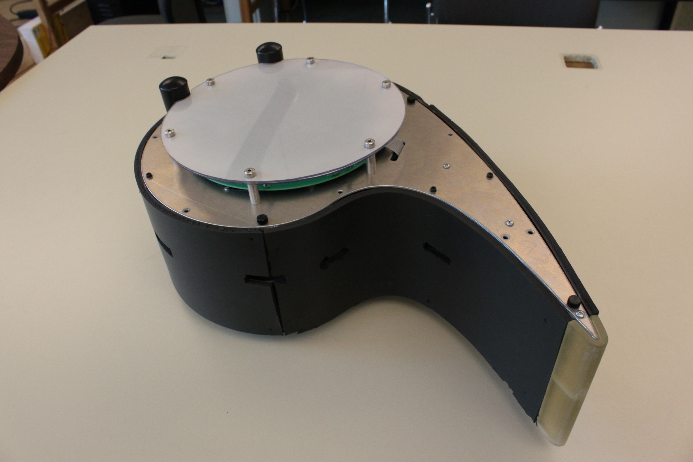
We investigated the practicality of nexting on the Critterbot, a custom-designed robust and sensor-rich mobile robot platform (Figure 1, left). The robot has a diverse set of sensors and has holonomic motion provided by three omni-wheels. Sensors attached to the motors report the electrical current, the input motor voltage, motor temperature, wheel rotational velocities, and an overheating flag, providing substantial observability of the internal physical state of the robot. Other sensors collect information from the external environment. Passive sensors detect ambient light in several directions from the top of the robot in the visible and infrared spectrum. Active sensors emit infrared light and measure the reflectance, providing information about the distance to nearby obstacles. Other sensors report acceleration, rotation, and the magnetic field. In total, we consider 53 different sensor readings, all normalized to values between 0 and 1 based on sensor limits.
For our experiments, the agent’s state representation was a binary vector, , with a constant number of 1 features, constructed by tile coding (see Sutton & Barto 1998). The features provided no history and performed no averaging of sensor values. The sensory signals were partitioned based on sensor modalities. Within each sensor modality, each individual sensor (e.g., Light0) has multiple overlapping tilings at random offsets (up to 8 tilings), where each tiling splits the sensor range into disjoint intervals of fixed width (up to 8 intervals). Additionally, pairs of sensors within a sensor modality were tiled together using multiple two-dimensional overlapping grids. Pairs of sensors were jointly tiled if they were spatially adjacent on the robot (e.g., IRLight with IRLight) or if there was a single sensor in between them (e.g., IRDistance1 with IRDistance3, IRDistance2 with IRDistance4, etc.). All in all, this tiling scheme produced a feature vector with components, most of which were 0s, but exactly 457 of which were 1s, including one bias feature that was always 1.
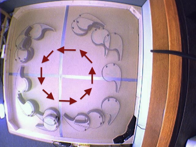
The robot experiment was conducted in a square wooden pen, approximately two meters on a side, with a lamp on one edge (see Figure 1). The robot’s actions were selected according to a fixed stochastic wall-following policy. This policy moved forward by default, slid left or right to keep a side IRDistance sensor within a bounded range (50-200), and drove backward while turning when the front IRDistance sensor reported a nearby obstacle. The robot completed a loop of the pen approximately once every 40 seconds. Due to overheating protection, the motors would stop to cool down at approximately 14 minute intervals. To increase the diversity of the data, the policy selected an action at random with a probability . At every time step (approximately 100ms), sensory data was gathered and an action performed. This simple policy was sufficient for the robot to reliably follow the wall for hours, even with overheating interruptions.
The wall-following policy, tile-coding, and the TD() learning algorithm were all implemented in Java and run on a laptop connected to the robot by a dedicated wireless link. The laptop used an Intel Core 2 Duo processor with a 2.4GHz clock cycle, 3MB of shared L3 cache, and 4GB DDR3 RAM. The system garbage collector was called on every time step to reduce variability. Four threads were used for the learning code. For offline analysis, data was also logged to disk for 120000 time steps (3 hours and 20 minutes).
4 Results
We applied TD() to learn 2160 predictions in parallel. The first 212 predictions had the target signal, , set to the sensor reading of one of the 53 sensors and the discount rate, , set to one of four timescales; the remaining 1948 predictions had the target signal set to one of 487 randomly selected components of the feature vector and the discount rate set to one of four timescales. The discount rates were one of the four values in , corresponding to time scales of approximately 0.1, 0.5, 2, and 8 seconds respectively. The learning parameters were and . The initial weight vector was set to zero.
Our initial performance question was scalability, in particular, whether so many predictions could be made and learned in real time. We found that the total computation time for a cycle under our conditions was 55ms, well within the 100ms duty cycle of the robot. The total memory consumption was 400MB. Note that with faster computers the number of predictions or the size of the weight and feature vectors could be increased at least proportionally. This strategy for nexting should be easily scalable to millions of predictions with foreseeable increases in parallel computing power over the next decade.
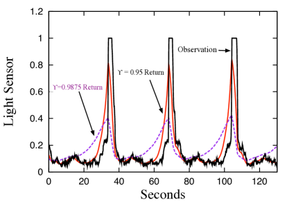
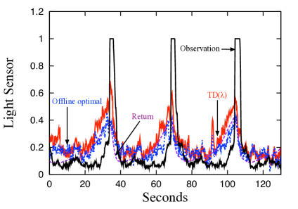
For an initial assesment of accuracy, let us take a close look at one of the predictions, in particular, at the prediction for one of the light sensors. Notice that there is a bright lamp in the lower left corner of the pen in Figure 1 (right). On each trip around the pen, the light sensor increases to its maximal level and then falls back to a low level, as shown by the black line in Figure 2. If the state features are sufficiently informative, then the robot may be able to anticipate the rising and falling of this sensor value. The ideal prediction is the return , shown on the left in the colored lines in Figure 2 for two time scales (two seconds and eight seconds). Of course, to determine these lines, we had to use the future values of the light sensor; the idea here is to approximate these ideal predictions (as in Equation 5) using only the sensory information available to the robot in its feature vector. The second panel of the figure shows the predictions due to the weight vector adapted online by TD() and due to the optimal weight vector, , computed offline (both for the 8-second time scale). The key result is that the robot has learned to anticipate both the rise and fall of the light. Both the learned prediction and the optimal offline prediction match the return closely, though with substantial noisy perturbations.
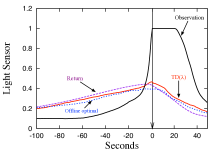
Figure 3 is a still closer look at this same prediction, obtained by averaging over 100 circuits around the pen, aligning each circuit’s data so that the time of initial saturation of the light sensor is the same. We can now see very clearly how the predictions and returns anticipate both the rise and fall of the sensor value, and that both the TD() prediction and the optimal prediction, when averaged, closely match the return.
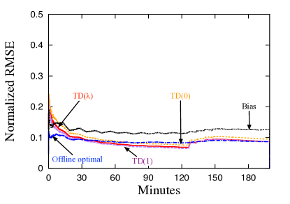
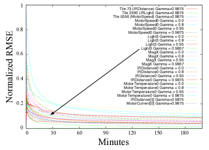
Having demonstrated that accurate prediction is possible, we now consider the rate of learning in Figure 4. The graphs shows that learning is fast in terms of data (despite the large number of features), converging to solutions with low error in the familiar exponential way. This result is important as is demonstrates that learning online in real time is possible on robots with a few hours of experience, even with a large distributed representation. For contrast, we also show the learning curve for a trivial representation consisting only of a bias unit (the single feature that is always 1). The comparison serves to highlight that large informative feature sets are beneficial. The comparison to the predictive performance of the offline-optimal solution shows a vanishing performance gap by the end of the experiment. The second panel of the figure shows a similar pattern of decreasing errors for a sample of the 2160 TD() predictions, showing that learning many predictions in parallel yields similar results. A noteworthy result is that the same learning parameters and representation suffice for learning answers to a wide variety of nexting predictions without any convergence problems. Although the answers continue to improve over time, the most dramatic gains were achieved after 30 minutes of real time.
5 Discussion
These results provide evidence that online learning of thousands of nexting predictions on a robot in parallel is possible, practical, and accurate. Moreover, the predictive accuracy is reasonable with just a few hours of robot experience, no tuning of algorithm parameters, and using a single feature representation for all predictions. The parallel scalability of knowledge-acquisition in this approach is substantially novel when compared with the predominately sequential existing approaches common for robot learning. These results also show that online methods can be competitive in accuracy with an offline optimization of mean squared error.
The ease with which a simple reinforcement learning algorithm enables nexting on a robot is somewhat surprising. Although the formal theories of reinforcement learning sometimes give mathematical guarantees of convergence, there is little guidance for the choice of features for a task, for selecting learning parameters across a range of tasks, or for how much experience is required before a reinforcement learning system will approach convergence. The experiments show that we can use the same features across a range of tasks, anticipate events before they occur, and achieve predictive accuracy approaching that of an offline-optimal solution with a limited amount of robot experience.
6 More General Nexting
The exponentially discounted predictions that we have focused on in this paper constitute the simplest kind of nexting. They are a natural first kind of predictive knowledge to be learned. Online TD-style algorithms can be extended to handle a much broader set of predictions, including time-varying choices of , time-varying , and even off-policy prediction (Maei & Sutton 2010). It has even been proposed that all world knowledge can be represented by a sufficiently large and diverse set of predictions (Sutton 2009).
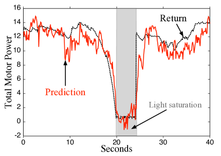
As one example of such an extension, consider allowing the discount rate to vary as a function of the agent’s state. The algorithmic modifications required are straightforward. In the definition of the return in Equation 1, is replaced with . In Equation 3, is replaced with and finally, in Equation 4, is replaced with . Using the modified definitions, the robot can predict how much motor power it will consume until either the light sensor is saturated or approximately two seconds elapse. This prediction can be formalized by setting the prediction’s target signal to be the sum of instantaneous power consumption of each wheel, () and throttling gamma when the light sensor is saturated ( when the light sensor is saturated and otherwise). The plots in Figure 5 shows that the robot has learned to anticipate how much power will be expended prior to reach the light or spontaneously terminating.
7 Conclusions
We have demonstrated multi-timescale nexting on a physical robot; thousands of anticipatory predictions at various time-scales can be learned in parallel on a physical robot in real-time using a reinforcement learning methodology. This approach uses a large feature representation with an online learning algorithm to provide an efficient means for making parallel predictions. The algorithms are capable of making real-time predictions about the future of the robot’s sensors at multiple time-scales using the computational horsepower of a laptop. Finally, and key to the practical application of our approach, we have shown that a single feature representation and a single set of learning parameters are sufficient for learning many diverse predictions. A natural direction for future work would be to extend these results to more general predictions and to control.
Acknowledgements
The authors thank Mike Sokolski for creating the Critterbot and Patrick Pilarski and Thomas Degris for preparation of Figure 1 and for essential assistance with the experiment briefly reported in Section 6. This work was supported by grants from Alberta Innovates – Technology Futures, the National Science and Engineering Reseach Council of Canada, and the Alberta Innovates Centre for Machine Learning.
References
Brogden, W. (1939). Sensory pre-conditioning. Journal of Experimental Psychology 25(4):323–332.
Butz, M., Sigaud, O., Gérard, P., Eds. (2003). Anticipatory Behaviour in Adaptive Learning Systems: Foundations, Theories, and Systems, LNAI 2684, Springer.
Carlsson, K., Petrovic, P., Skare, S., Petersson, K., Ingvar, M. (2000). Tickling expectations: neural processing in anticipation of a sensory stimulus. Journal of Cognitive Neuroscience 12(4):691–703.
Clark, A. (in press). Whatever Next? Predictive Brains, Situated Agents, and the Future of Cognitive Science. Behavioral and Brain Sciences.
Dayan, P., Hinton, G. (1993). Feudal reinforcement learning. Advances in Neural Information Processing Systems 5, pp. 271–278.
Gilbert, D. (2006). Stumbling on Happiness. Knopf Press.
Grush, R. (2004). The emulation theory of representation: motor control, imagery, and perception. Behavioural and Brain Sciences 27:377–442.
Hawkins, J., Blakeslee, S. (2004). On Intelligence. Times Books.
Huron, D. (2006). Sweet anticipation: Music and the Psychology of Expectation. MIT Press.
Kaelbling, L. (1993). Learning to achieve goals. In Proceedings of International Joint Conference on Artificial Intelligence.
Levitin, D. (2006). This is Your Brain on Music. Dutton Books.
Pavlov, I. (1927). Conditioned Reflexes: An Investigations of the Physiological Activity of the Cerebral Cortex, translated and edited by G. V. Anrep. Oxford University Press.
Pezzulo, G. (2008). Coordinating with the future: The anticipatory nature of representation. Minds and Machines 18(2):179–225.
Rescorla, R. (1980). Simultaneous and successive associations in sensory preconditioning. Journal of Experimental Psychology: Animal Behavior Processes 6(3):207–216.
Singh, S. (1992). Reinforcement learning with a hierarchy of abstract models. Proceedings of the Conference of the Association for the Advancement of Artificial Intelligence (AAAI-92), pp. 202–207.
Sutton, R. S. (1988). Learning to predict by the method of temporal differences. Machine Learning 3:9–44.
Sutton, R. S. (1990). Integrated architectures for learning, planning, and reacting based on approximating dynamic programming, Proceedings of the Seventh International Conference on Machine Learning, pp. 216–224.
Sutton, R. S. (1995). TD models: Modeling the world at a mixture of time scales. Proceedings of the International Conference on Machine Learning, pp. 531–539.
Sutton, R. S. (2009). The grand challenge of predictive empirical abstract knowledge. In: Working Notes of the IJCAI-09 Workshop on Grand Challenges for Reasoning from Experiences.
Sutton, R. S., Barto, A. G. (1990). Time-derivative models of Pavlovian reinforcement. In Learning and Computational Neuroscience: Foundations of Adaptive Networks, pp. 497–537. MIT Press.
Sutton, R. S., Barto, A. G. (1998). Reinforcement Learning: An Introduction. MIT Press.
Sutton, R. S., Modayil, J., Delp, M., Degris, T., Pilarski, P. M., White, A., Precup, D. (2011). Horde: A scalable real-time architecture for learning knowledge from unsupervised sensorimotor interaction. Proceedings of the 10th International Conference on Autonomous Agents and Multiagent Systems, pp. 761–768.
Sutton, R. S., Precup, D., Singh, S. (1999). Between MDPs and semi-MDPs: A framework for temporal abstraction in reinforcement learning. Artificial Intelligence 112:181–211.
Tolman, E. C. (1951). Purposive Behavior in Animals and Men. University of California Press.
Wolpert, D., Ghahramani, Z., Jordan, M. (1995). An internal model for sensori-motor integration. Science 269(5232):1880–1882.