The power spectrum from the angular distribution of galaxies in the CFHTLS-Wide fields at redshift 0.7
Abstract
We measure the real-space galaxy power spectrum on large scales at redshifts 0.5 to 1.2 using optical colour-selected samples from the CFHT Legacy Survey. With the redshift distributions measured with a preliminary 14000 spectroscopic redshifts from the VIMOS Public Extragalactic Redshift Survey (VIPERS), we deproject the angular distribution and directly estimate the three-dimensional power spectrum. We use a maximum likelihood estimator that is optimal for a Gaussian random field giving well-defined window functions and error estimates. This measurement presents an initial look at the large-scale structure field probed by the VIPERS survey. We measure the galaxy bias of the VIPERS-like sample to be () on scales averaged over . We further investigate three photometric redshift slices, and marginalising over the bias factors while keeping other CDM parameters fixed, we find the matter density .
keywords:
cosmological parameters, observations, large-scale structure of Universe, methods: statistical1 Introduction
The shape of the galaxy clustering power spectrum encodes the dynamical history of the Universe under the influence of baryons, dark matter and dark energy. On large scales the assumption of Gaussianity can be made, and the statistic summarises all of the cosmological information that is available.
Measurements of the power spectrum at have led to fundamental tests of the CDM model (Tegmark et al., 2004; Efstathiou et al., 2002). The angular distribution of galaxies on the sky, although less sensitive than the full three-dimensional view, has played an important role as well. Indeed, strong tests of the CDM model were made with the two-dimensional correlation function from the APM galaxy survey (Maddox et al., 1990). Photometric surveys have the capability to probe significantly larger volumes at higher sampling rates than targeted spectroscopic surveys. The advantages have become clear with the advancement of photometric redshift estimation methods. The loss in three-dimensional precision can be compensated for with increased statistics leading to strong cosmological constraints that are comparable to the results from spectroscopic surveys.
Additionally, the projected density field is only weakly sensitive to redshift-space distortions, thus it provides a means to infer the real-space power spectrum directly. The dependence on peculiar velocities becomes important for narrow redshift slices and can be turned into a useful measure of the growth rate (Ross et al., 2011a). Measurements of the baryon acoustic feature and redshift-space distortions have now been made on photometric samples taken from the Sloan Digital Sky Survey (Padmanabhan et al., 2007; Blake et al., 2007; Thomas, Abdalla & Lahav, 2011).
In this analysis, we present a new measurement of the real-space galaxy power spectrum using a photometric catalogue of galaxies at from the Canada-France-Hawaii Telescope Legacy Survey (CFHTLS) Wide survey. The survey consists of four fields covering a total area of 133 . The extent of the largest field, W1, is or at z=0.7, giving a maximum scale we may probe of . The dataset has been used for previous cosmological analyses, in particular for weak lensing (Fu et al., 2008; Kilbinger et al., 2009; Tereno et al., 2009; Shan et al., 2011) and galaxy correlation function measurements (Coupon et al., 2011).
A key ingredient needed to interpret the projected density field and constrain the three-dimensional power spectrum is the redshift distribution of the galaxy sample. For this we use spectroscopy from the VIMOS Public Extragalactic Survey111VIPERS website: vipers.inaf.it (VIPERS)(Guzzo et al., 2011). VIPERS is an ongoing spectroscopic program to target galaxies in the redshift range 0.5-1.2 in a total area of 24 in the CFHTLS W1 and W4 fields. The accuracy of the spectroscopic measurements from VIPERS provide an unbiased estimate of the redshift distribution. With this knowledge, we are confident that we can deproject the angular clustering signal and constrain the three dimensional power spectrum. The primary advantage of studying the deprojected power spectrum is its closeness to theory. The shape of the angular power spectrum is complicated by its dependence on survey properties, its depth and geometry. Furthermore, in projection, scales are mixed. Ideally we would like to separate the power on large scales in the linear regime from power on small scales that is influenced by complex astrophysical processes.
How to derive the three-dimensional power spectrum from the two-dimensional density field is a problem of deconvolution. A good inversion method should be stable against noise in the data. Preliminary work done by Baugh & Efstathiou (1993, 1994) and Gaztañaga & Baugh (1998) used the Lucy deconvolution method that is known to be robust. To further derive cosmological constraints, we must be able to estimate the covariance of the deprojection. Methods of propagating the error from the angular correlation function to the three-dimensional power spectrum were developed by Dodelson & Gaztañaga (2000) who perform the inversion with a prior on the smoothness of the power spectrum and compute a covariance matrix of the estimate. Further work by Eisenstein & Zaldarriaga (2001), Dodelson et al. (2002) and Maller et al. (2005) made use of the singular-value decomposition technique to remove modes that destabilise the inversion.
Importantly, the deprojection method should produce well-defined window functions that describe the mode mixing. The aim is to separate the small and large scales that are mixed in projection, and the residual leakage should be understood. A similar problem was solved with the maximum likelihood methods developed for the cosmic microwave background angular power spectrum (Tegmark, 1997; Bond, Jaffe & Knox, 1998) and then later applied to galaxy surveys (Huterer, Knox & Nichol, 2001; Tegmark et al., 2002). Applications to the deprojection of the power spectrum were presented by Efstathiou & Moody (2001) and Szalay et al. (2003).
In this work, we adopt the maximum-likelihood technique to construct an estimator for the power spectrum. The result is optimal under the assumption that the density is represented by a Gaussian random field. This is a reasonable assumption for the galaxy distribution on large scales. Moreover, the estimator also simultaneously gives the covariance of the estimate as well as the window functions. For small surveys, where the window functions must be handled carefully, the approach is especially useful. We pay close attention to the window functions for the results presented here. Maximum likelihood estimates are computationally expensive. However, because of the relatively small field sizes we consider, we can perform all computations on a consumer level four-core desktop computer.
In this article, we first introduce the CFHTLS and VIPERS datasets used. In Sections 3 and 4 we review the angular power spectrum formalism and the maximum likelihood deprojection using a quadratic estimator. We then apply the method to Gaussian simulations and investigate potential biases due to uncertainty in the redshift distribution and the fiducial cosmology. Lastly, we measure the power spectrum with CFHTLS data and constrain the linear galaxy bias and matter density.
We report magnitudes using the AB magnitude convention in the CFHT photometric system. We assume a flat CDM cosmology with , , , and (Larson et al., 2011).
2 Data
2.1 Photometric selection
The Canada-France-Hawaii Telescope Legacy Survey (CFHTLS) Wide includes four fields labelled W1, W2, W3 and W4. The total area is 133 imaged with five-band photometry to a depth of . We construct colour-selected galaxy samples from these fields to match the spectroscopic target selection used by the VIMOS Public Extragalactic Survey (VIPERS).
VIPERS is a spectroscopic program to measure the redshifts of galaxies over an area of 24 in the CFHTLS W1 and W4 fields. Galaxies are targeted from CFHTLS-Wide photometry to a flux limit of with colour criteria to produce a sample at having few low-redshift interlopers. The selection is done in the , colour plane with the following limits on extinction-corrected magnitudes: (1) AND OR (2) AND (Guzzo et al., 2011). We replicate these colour criteria on the full CFHTLS-Wide photometry T0006 release (Goranova et al., 2009). Hereafter, we refer to this selection as the VIPERS-like sample.
Every source has an estimated photometric redshift and star-galaxy classification from the T0006 photometric redshift catalogue. The star-galaxy classification accounts for both the source profile and fits to stellar spectral templates (Coupon et al., 2009). We apply the same criteria as used for the VIPERS target selection and exclude all sources photometrically classified as stars (7% of sources). From the remaining sample identified as galaxies, we remove sources that fail to fit galaxy spectral templates with reduced . This cut removes sources with incomplete or spurious photometry amounting to 0.15% of sources which are typically near to the edges of masked regions, bright stars or field borders.
We also use the photometric redshifts to select sub-samples of narrower slices in redshift, labelled S6 (), S7 () and S8 (), see Table 2. As with the VIPERS-like sample, these are also limited to . We have confirmed that these photometric redshift selections at also meet the VIPERS selection criteria. Thus, the VIPERS spectroscopy can be used to calibrate the redshift distributions of these samples without introducing a bias.
The VIPERS spectroscopic targets were selected from the CFHTLS T0005 catalogue after field-to-field colour corrections were applied by the VIPERS team. These colour corrections are no longer necessary in the T0006 update, and it has been shown that the selections from the two catalogue versions match well (Guzzo et al., 2011). We note that a limited area in the CFHTLS has been observed with a replacement -band filter called . The photometric redshifts were computed with the appropriate filter transmission function. To construct our limited samples, we take a reasonable approach and do not distinguish between the two bands.
The CFHTLS catalogues also include corrections for Galactic extinction. We do not consider residual systematic effects of reddening here because all four fields have relatively low and uniform extinction at the level of in W4 and in the other fields. The limit is 2 magnitudes brighter than the detection limit of the survey, thus we do not expect the selection to be affected by the extinction correction.
a)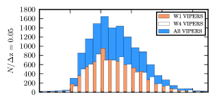 b)
b)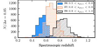
2.2 Density maps
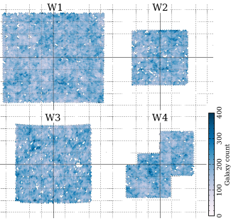
We construct the density maps for the photometrically-selected samples by counting galaxies in cells defined by the Healpix scheme with a resolution of 7′ () (Górski et al., 2005). The maps for the VIPERS-like colour selection are shown in Fig. 1. We use a survey mask provided by CFHTLS and exclude sources that fall within the halos of bright stars. For cells that fall on a mask boundary, we measure the fractional coverage using a uniformly spaced grid of test points within the cell. We use Mangle2 to test if points fall inside the mask (Swanson et al., 2008). This provides us with a weight map where is the fractional sampling for pixel . Cells that have less than 50% inclusion in the survey are removed from the map. The areas of the four fields W1, W2, W3 and W4 are 57.7, 18.6, 36.8, 19.6 . After putting galaxies in the Healpix cells, the number of pixels in the four maps are: 4787, 1592, 3045 and 1651.
With galaxies counted in cell , the over-density is computed with . The mean density in a cell, , is computed from all four fields as . The variance of , assuming Poisson statistics, is .
The clustering of foreground stars can be a significant source of systematic error on large angular scales (Ross et al., 2011a). For the CFHTLS, we can estimate the stellar contamination rate independently in each of the four fields and apply local corrections to the galaxy density. We measure the contamination rate directly in the W1 and W4 fields by counting the number of targets spectroscopically classified as stars in the VIPERS sample. We then extrapolate these rates to the W2 and W3 fields by computing the fraction of sources photometrically classified as stars and then scaling.
The total counts in a cell broken down into stars and galaxies is given by , and the stellar contamination fraction is . The values we derive are listed in Table 2. We apply the correction in the following way: and (Huterer, Knox & Nichol, 2001). The effect on the amplitude of the power spectrum is %.
A fraction of galaxies will also be misclassified as stars and removed from the sample. However, as long as the sample is representative of the full population, the power spectrum measurement will not be biased. This may not be the case in reality since misclassified galaxies may preferentially represent a subclass with a different power spectrum amplitude. We do not investigate this correction here.
| Sample | ||||
|---|---|---|---|---|
| SV: VIPERS-like | 0.70 | 13191 | 1870617 | 14099 |
| S6: | 0.56 | 2548 | 340611 | 2567 |
| S7: | 0.69 | 4969 | 613643 | 4628 |
| S8: | 0.84 | 3030 | 416897 | 3142 |
| Sample | W1 | W2 | W3 | W4 |
|---|---|---|---|---|
| SV | 0.019 | 0.056 | 0.020 | 0.044 |
| S6 | 0.013 | 0.030 | 0.010 | 0.017 |
| S7 | 0.015 | 0.042 | 0.015 | 0.032 |
| S8 | 0.017 | 0.055 | 0.019 | 0.048 |
2.3 Redshift distribution
We use the VIPERS spectroscopic redshift catalogue (internal release, version 1.1) to calibrate the redshift distribution of the photometric samples, see Table 2. In total, we use 13191 galaxies from VIPERS including 6516 from the W1 field and 6675 from the W4 field. All targets that meet the photometric selection criteria with secure redshifts are used. We select based on the quality flag zflag. Reliable redshifts have , and we take (galaxy type), (AGN type) and (serendipitous detections). The flag also has a fractional part indicating agreement with the photometric redshift on a scale from 1 to 5, where 5 indicates good agreement (within ).
We estimate the redshift distribution from the histogram of spectroscopic redshifts with a bin size of , see Fig. 2. We use the histograms directly in the analysis with linear interpolation between bin centres. The redshift distribution of the W1 and W4 samples are remarkably similar despite that these fields are well separated on the sky. We use the distributions from the two fields to test the impact of cosmic variance on our results. As we will conclude in Section 5.1, small perturbations to the redshift distribution do not strongly impact the results.
The selection function of the VIPERS survey is not uniform with target apparent flux. There are two sampling rates that we consider: first, the fraction of potential targets that are selected for observation, and second, the fraction of observed targets that give a successful redshift measurement. The first distribution is nearly uniform; the VIMOS spectrograph can place slits on 40% of the potential targets and this fraction is found to be independent of the magnitude of the source. However, we do find that the fraction of targets that have a measured redshift with qualities meeting our criteria drops from 100% at to 50% at , the flux limit of the survey. This trend may be corrected for by weighting the contribution of each galaxy in the redshift distribution by the inverse of the sampling rate. However, we find that the correction has a negligible effect on the distribution. Weighting the galaxies shifts the mean redshifts of the samples by less than . We also confirm that lowering the quality threshold of the spectroscopic sample to , which adds 11% additional sources, does not significantly alter the distribution. In Section 5.1 we consider the effect of shifting the mean redshift by to provide an overly-conservative check on the effect of uncertainties in the redshift distribution.
3 Angular Power Spectrum
From galaxy counts in an image we may infer the projected over-density of galaxies on the sky, . Typically this is an integration through a broad slice in redshift defined by a photometric galaxy selection function or simply by the limiting flux of the survey. We expand the density field in spherical harmonics and express the power in mode by the spectrum .
We may write the angular power spectrum as a projection of the three-dimensional power spectrum, . On large scales, the power spectrum evolves with the linear growth factor, . We scale the power spectrum taken at the median redshift of the sample, , as . This gives,
| (1) |
where is comoving distance. In the small angle approximation, the spherical Bessel function can be approximated as , expressed with a Dirac delta function, and we find Limber’s equation:
| (2) |
The projection kernel, , is given by,
| (3) |
A correction may be added to account for redshift space distortions although it is sizable only on large scales at that we are not sensitive to here (Thomas, Abdalla & Lahav, 2011; Ross et al., 2011b). We may now approach the deprojection problem as a deconvolution of Limber’s equation.
4 Power spectrum estimator
On large scales, the galaxy density may be described by a Gaussian random field and the distribution is fully characterised by its variance. With this assumption, the likelihood function of the observed overdensities on the sky may be written explicitly. We order the pixels of the density map and form a data vector, , and write the covariance of the data as . The likelihood function is,
| (4) |
The covariance between the overdensity in pixels and separated by an angle is given by the sum of the signal and the noise components,
| (5) |
where is the noise covariance matrix and are Legendre polynomials. The noise matrix is taken to be diagonal with Poisson elements given by . The finite resolution of the pixelised map attenuates the power spectrum by the pixel window function, , which depends on the pixel geometry (Górski et al., 2005).
We now derive a power spectrum estimator that maximises the likelihood function, . The quadratic form was introduced by Tegmark (1997) and explicit derivations have been given in Dodelson (2003, Ch. 11), Dahlen & Simons (2008) and Bond, Jaffe & Knox (1998). We give an overview here, since many variations exist.
We denote the set of parameters to be estimated by the vector . For our study, will represent a bin of the power spectrum. We begin with an initial estimate, , and intend to use an optimisation algorithm to find a better estimate, , that maximises the likelihood function. With the assumption that has a quadratic form near the peak, we may apply the Newton-Raphson root-finding method to move toward the peak of the likelihood function (Press et al., 1992), with,
| (6) |
This expression may be used iteratively to locate the peak.
We evaluate the derivative terms in Appendix A, and now simply state the final result for one iteration step:
| (7) |
| (8) |
The matrix is a mixing matrix that sets the normalisation and may be specified to form linear combinations of the bin estimates. We will use this matrix to shape the window functions. The second term in Eq. 7 subtracts the noise bias.
We see that the estimator weights the data by their covariance: . This approach has the favourable property that spatial modes contribute to the measurement with an inverse-variance weight. The weighting also appropriately ‘tapers’ the map near the mask boundary giving compact window functions in harmonic space.
We have not yet specified the parameter vector . We set to bins of the three-dimensional power spectrum and evaluate the derivative matrix in Eq. 8, as,
| (9) |
Here, we have replaced the integral in Limber’s equation (Eq. 2) with a discrete sum over with logarithmic bin width .
The expectation of the estimate is given by,
| (10) |
where we have introduced the Fisher matrix,
| (11) |
The variance of the estimate is,
| (12) |
and the window functions are .
The inverse of the Fisher matrix represents the minimum variance that we may hope to achieve on . With we see that we have an estimator that is optimal in the sense that it is unbiased and has minimum variance (Tegmark, 1997). This approach may not be practical however, because the Fisher matrix is often singular or numerically ill-conditioned. Intuitively, this reflects the fundamental limit that we cannot probe the power spectrum at scales smaller than where is the angular size of the survey.
Instead, we choose with the aim of diagonalising the covariance matrix. By factoring the Fisher matrix as , we can set . The covariance matrix is now . In practice, we compute as the square root of the Fisher matrix using a singular value decomposition (SVD) method. We also rescale to normalise the window functions such that . This approach was shown by Tegmark (1997) to result in sharper window functions than the common choice for , a diagonal matrix with .
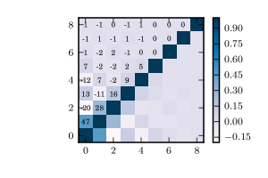
We find that the matrix is ill-conditioned when the window functions are broad, especially for the SV sample which has a wide redshift distribution. To find a stable inversion, we use a pseudo-inverse technique by keeping only the largest singular values. The consequence of using a pseudo inverse is that the covariance matrix will not be perfectly diagonalised. The covariance matrix for the VIPERS estimate after carrying out this operation is shown in Fig. 3. The choice of how many modes to keep in the pseudo-inverse affects the shape of the window functions and the scales that are probed. We find that the smaller singular values probe large scales, in the same fashion as in the SVD analyses by Eisenstein & Zaldarriaga (2001) and Maller et al. (2005). We set the scale ensuring that the resulting window functions are positive and reach the largest scales available to the survey.
The estimate and covariance model depend on the chosen fiducial cosmology through the form of the likelihood function and the projection kernel. Both the shape and normalisation of the power spectrum can be important. Although the normalisation cancels in the estimator (neglecting the noise term), it is important for the Fisher matrix and covariance. For these reasons, maximum likelihood estimators are often applied iteratively to arrive at consistent results. We explore these dependencies with simulations in the next section.
a)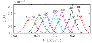 b)
b)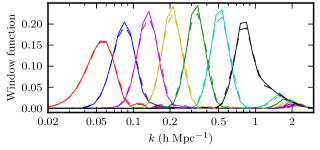
a)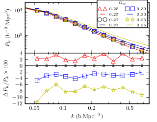 b)
b)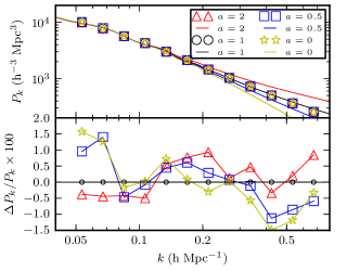
5 Simulations
5.1 Gaussian realisations
As a test of the method, we estimate the power spectrum for Gaussian realisations of the projected density field. The simulations are constructed using a CAMB power spectrum with the Halofit model (Lewis, Challinor & Lasenby, 2000; Smith et al., 2003) and projected through the VIPERS redshift distribution. With these , we use Healpix Synfast to generate simulated density maps. We produced 1000 independent maps with a resolution of 7′ (). We add noise fluctuations by drawing from a Gaussian distribution assuming a variance given by Poisson statistics with galaxies/cell. This is a higher level of noise than we find in the CFHTLS catalogue. For the geometry of the mock survey, we use the actual survey mask of the W2 field. It includes 1592 pixels covering 21 .
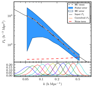
We compute the Fisher matrix in logarithmic bins from with . The results are plotted in Fig. 4. The data points are re-binned to and plotted from . The corresponding window functions are shown in the bottom panel. The data are plotted at the peaks of the window functions. On large and small scales, the window functions begin to overlap and converge as the limits set by the survey geometry are reached. On small scales, we see a secondary peak in the window function at which arises from the pixel scale of the map, see Fig. 5.
We convolve the theory power spectrum with the window functions and find that the mean of the Monte Carlo runs agrees well within a few percent. We expect that the precision is limited by the finite binning of the Fisher matrix and truncation of the window functions, but these effects are well below the statistical uncertainties. The errors computed analytically from the Fisher matrix agree with the distribution of Monte Carlo runs to within a few percent. These errors are for a single field, and so, we can expect to achieve a factor of two better with the combination of four fields.
5.2 Dependence on redshift distribution
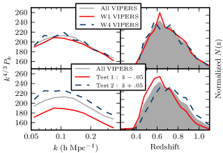
We checked the robustness of the measurement to uncertainties in the redshift distribution by repeating the analysis with different assumed distributions. The simulations were generated with the measured redshift distribution from the complete VIPERS sample, and we first re-analysed them with distributions derived from two subsamples, the redshift distribution of W1 and W4. The numbers of spectra taken in the two fields are similar and the spectroscopy covers similar areas, but, the fields are widely separated on the sky and so any differences could be attributed to cosmic variance. We compute the Fisher matrix using the two distributions and find that the projection kernels and window functions agree (Fig. 5). The bias introduced by a mismatched redshift distribution is at the percent level, below the statistical errors.
Additionally, the measured redshift distribution could be inaccurate due to sampling biases in the VIPERS survey. In Section 2.3, we concluded that the uncertainty in the mean redshift of the distribution, , is known to better than . As an overly conservative check, we examine the consequences of shifting the redshift distribution by . This was done by modulating the measured distribution of the full VIPERS sample by the linear function . The modified distributions have and , while the original sample has , see the lower panel of Fig. 6. We find that reducing by 7% lowered the derived power spectrum by 10%. Increasing by 7% increased the power spectrum by 6%. This large shift in would thus lead to a systematic error in the estimated bias factor at the level of %.
5.3 Dependence on fiducial cosmology
The dependence on the fiducial cosmology enters the analysis in two ways. First, we rely on the cosmology to model the likelihood function. In the maximum likelihood estimator, the data covariance matrix plays the role of a weight. Modifying the fiducial power spectrum changes the weighting function and could bias the estimator. We can expect that assuming the wrong matter density for example, could bias the estimator and make the variance properties sub-optimal.
The second dependence on the fiducial cosmology is through the projection kernel. In the previous section, we discussed how shifting the redshift distribution affects the amplitude of the power spectrum estimate. We can expect that varying the cosmology and the redshift-distance relation will have a similar effect.
Our Gaussian simulations were constructed using the reference CDM power spectrum with the Halofit model. To test the dependence on the cosmology, we first re-analyse the maps using fiducial power spectra with different assumed values of the matter density, taking , 0.30 and 0.35. All other parameters were held fixed at the reference values. We find that despite assuming the wrong matter density, we recover the correct shape of the power spectrum from the mean of 1000 simulation runs to within 2%, see Fig. 7, Panel a. However, it is clear that the amplitude is strongly biased. This is due to the dependence of the projection kernels on . This geometric dependence on the background cosmology dominates over any bias in the estimator due to sub-optimal weighting. These findings support an iterative approach.
Next, we check the influence of variations in the amplitude of the power spectrum at small scales. The shape of the power spectrum on small scales has developed with the aid of n-body simulations but it remains a source of systematic uncertainty. We vary the small-scale amplitude using an interpolation parameter :
| (13) |
We test a range of amplitudes with ( gives the Halofit model). We find that the estimator is remarkably robust, see Fig. 7, Panel b. The discrepancy introduced by the variation in the small-scale amplitude is less than on large scales and it is dominated by numerical uncertainties up to . This supports the conclusion that using sub-optimal weights does not significantly bias the result.
6 Results
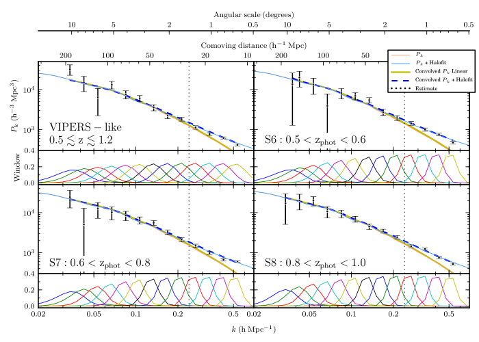
We now carry out the estimation of the power spectrum on the CFHTLS data for the VIPERS-like sample and three photometric redshift subsamples, see Fig. 8. For the analysis, a fiducial CAMB power spectrum with the Halofit model is assumed. The Fisher matrix is computed with 60 bins logarithmically spaced from with . We use a wide -range to map out the window functions but all these data are not useful for analysis. We restrict the study to 13 points from . We can go to smaller scales, although the Gaussian error estimate will not be appropriate. We use a bin size of which is appropriate choice considering the width of the survey window functions. The plotted error bars are derived from the diagonal elements of the covariance matrix found computed from Eq. 12.
For each field, we compute the normalised quantity from Eq. 7, , where indexes the fields 1-4, along with the Fisher matrix (Eq. 11). These results are then summed together, and the final combined estimate is computed by where normalised such that . This combination properly weights the data. The covariance of the estimate for the VIPERS-like sample is shown in Fig. 3. At low , neighbouring bins are nearly 50% correlated, but the matrix becomes more diagonal at larger . The limitation in diagonalising the covariance matrix comes in the inversion of . This is computed with a pseudo-inverse method. The inversion becomes easier for the narrower photometric redshift slices where a nearly perfect inversion is possible. The window functions are sharper for these redshift slices as well.
We do not run the maximum likelihood algorithm in an iterative fashion. The data do not support strong constraints on CDM parameters alone and we find that beginning with a fiducial CDM power spectrum, we have a very good fit to the data. This indicates that our starting point is already near to the peak of the (very broad) likelihood function. However, we do effectively carry out one iteration of the estimator to find the galaxy bias and set the amplitude of the fiducial power spectrum. This is necessary because the estimator and covariance do not simply scale linearly with amplitude in the presence of noise. A second run allows us to set the amplitude of the fiducial power spectrum ensuring that the error estimate is correct.
We compute a one-parameter fit to estimate the galaxy bias on linear scales. We restrict this fit to the first 9 points at . Given the measurements in vector and the convolved CDM model in vector , we find the amplitude, , that maximises the likelihood function, . The solution is given by,
| (14) |
with variance . The resulting values of the galaxy bias are listed in Table 4, where we have assumed a value of . The bias increases with redshift as expected for a flux limited survey. In fact, the amplitude of the power spectrum is not seen to change with increasing redshift, indicating that the evolution of the growth factor and the galaxy bias factors approximately cancel. We find an approximately constant error on the bias factor in each redshift range; this is simply due to the fact that the amplitude of the fiducial power spectrum (from which the errors are derived) is approximately constant.
Also in Table 4, we list the values at the best fit. The number of degrees of freedom is approximately 8. The values are lower than expected, specifically for S8 for which we find . Formally, the probability of finding with 8 degrees of freedom is . This could indicate that the covariances and, consequently the error bars, are over-estimated for this sample.

| Sample | ||
|---|---|---|
| VP: VIPERS-like | 7.2 | |
| S6: | 7.1 | |
| S7: | 5.7 | |
| S8: | 2.0 |
7 Parameter estimation
Before we may carry out a joint analysis, we must estimate the covariance between the overlapping photometric samples. We will estimate the covariance of the estimators with a Fisher matrix approach in the full-sky limit and then rescale to find the errors for our survey geometry.
We compute the covariance between two samples labelled and . To simplify the expression, we write the product of the kernel with the beam and integration step as, and the sum of the signal and noise covariance as, . It is more convenient to use the harmonic space representation, and we switch the data vector from to . The covariance matrix is diagonal: .
A component of the Fisher matrix for a single sample for two power spectrum bins, and is,
| (15) |
We can write the quadratic estimator for the power spectrum as,
| (16) |
We find the covariance between the two sample estimates to be,
| (17) | |||||
We scale by the fractional sky coverage of the survey, , which approximately accounts for the number of modes that may be probed. The small survey size also broadens the window functions, which we account for in the covariance with: .
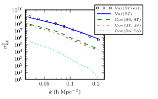
The variances for one sample computed with Eq. 17 in the full-sky limit match well with the full computation of the Fisher matrix (Eq. 12), see Fig. 9. Although, we find that the full-sky computation underestimates the variance by a factor of . This is not surprising since we have neglected the precise survey geometry. As a correction, we rescale the estimate to match the variance in the S7 slice. In Fig. 9 we also show the analytic estimates of the covariances between the three redshift slices that we may now use to perform a joint likelihood analysis.
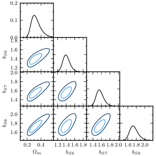
Using the sample covariances, we jointly estimate the linear galaxy bias factors of the three photometric redshift slices, S6, S7 and S8, labelled as , and along with . All other CDM parameters are held fixed and we set . We compute the likelihood of a model with the full covariance matrix. The fit is limited to the first 9 datapoints of each sample, giving a maximum of . We exhaustively evaluate the likelihood over the 4-dimensional parameter grid. Views of the likelihood surface, marginalised over pairs of parameters are shown in Fig. 10. The marginalised constraints are listed in Table 4 with 68% confidence intervals.
The joint analysis prefers a slightly higher value of , , versus the fiducial model with 0.272. Due to the correlations between parameters, this results in higher values of the galaxy bias factors than were found with the fiducial model fixed (Table 4).
8 Conclusions
The CFHTLS-Wide fields probe a significant cosmological volume at redshifts not reached by other galaxy surveys to date. We use the projected density field from photometric redshift samples to constrain the real-space power spectrum and derive constraints on the matter density and linear galaxy bias factors. These results are made possible by precise knowledge of the redshift distributions provided by preliminary results from the VIPERS survey.
The primary advantage of computing the power spectrum directly from the angular distribution, instead of using conventional spherical harmonics is that we may construct window functions in Fourier space. By optimising this, we achieve sharper constraints on the power spectrum than when we are limited to bands. This approach comes with the cost that we must adopt a fiducial power spectrum. We showed that using the wrong fiducial power spectrum, although leading to sub-optimal weights, does not significantly bias the estimate. This is true even on small scales, and we can effectively use this method to deconvolve small and large scales in Limber’s equation. Residual systematic error on the derived power spectrum is at the 1% level, well below the sensitivity of the measurement.
The deprojection does strongly depend on the assumed redshift distribution of the galaxy sample as well as the cosmology used to compute the redshift-distance relation. The cosmology dependence of the measurement makes the interpretation difficult, but to a first approximation, only the amplitude is affected; the shape of the power spectrum is recovered correctly. Thus, a converging iterative procedure can be implemented by updating the fiducial model and repeating the analysis.
There is a degeneracy between a shift in the assumed redshift distribution and the cosmological model. This is unavoidable when studying a field in projection. However, the constraints on the redshift distribution can always be improved with further observation. In our analysis, from the sampling biases present in the VIPERS spectroscopy, we estimate the uncertainty in the mean redshift to be at the 1% level. Thus, we do not expect a strong systematic error in the derived galaxy bias parameters. We do note that the observed trend of low values for the best-fit models in the higher redshift samples can arise if the covariance is overestimated. This could be a weak hint that the true mean redshift is lower than what we assume or that a modification is needed in the fiducial cosmology.
Recently, the galaxy bias was measured from the CFHTLS-Wide fields in the context of the halo model by Coupon et al. (2011). Our final two photometric redshift bins, S7 and S8, correspond with samples constructed by Coupon et al. so we are able to compare the resulting bias values. Coupon et al. constructed volume-limited samples using luminosity cuts resulting in a selection of brighter galaxies, thus we may expect their bias values to be larger. The halo model constraints of Coupon et al. (2011) give for S7, , and for S8, . These values have been scaled by 1.03 to transform from a cosmology with to which is assumed here. Our value of for the S7 sample is higher, while for the S8 sample it is lower, although both are in agreement with Coupon et al. within the 2 confidence limit. The measurements are based on different physical scales (Coupon et al. restrict the correlation function to angular scales ) and different model assumptions have been used. Thus it is reasonable to consider the measurements as independent estimates.
Our results provide a preliminary look at the large-scale structure field probed by the VIPERS colour selection and demonstrate the strengths of the VIPERS sample for clustering studies at . We anticipate promising results with the full VIPERS spectroscopic sample.
Acknowledgements
We are grateful to the VIPERS team for supporting this project. In particular, we thank Lauro Moscardini for suggestions that improved the work. We thank Jian-Hua He for carefully reading the manuscript. The computational methods used were inspired by István Szapudi’s mlhood code. Our results are derived with CosmoPy (www.ifa.hawaii.edu/cosmopy) and Healpix with Healpy (healpix.jpl.nasa.gov, code.google.com/p/healpy). We acknowledge the support of INAF through a PRIN 2008 grant. AP and KM have beed supported by the research grant of the Polish Ministry of Science Nr N N203 51 29 38. A part of this work was carried out within the framework of the European Associated Laboratory “Astrophysics Poland-France.” Based on data obtained with the European Southern Observatory Very Large Telescope, Paranal, Chile, program 182.A-0886. Based on observations obtained with MegaPrime/MegaCam, a joint project of CFHT and CEA/DAPNIA, at the Canada-France-Hawaii Telescope (CFHT) which is operated by the National Research Council (NRC) of Canada, the Institut National des Sciences de l’Univers of the Centre National de la Recherche Scientifique (CNRS) of France, and the University of Hawaii. This work is based in part on data products produced at TERAPIX and the Canadian Astronomy Data Centre as part of the Canada-France-Hawaii Telescope Legacy Survey, a collaborative project of NRC and CNRS.
Appendix A Quadratic estimator
In Section 4, we reasoned that we would apply the Newton-Raphson root-finding algorithm (Eq. 6) to locate the peak of the likelihood function (Eq. 4). We now continue and evaluate the derivatives of the likelihood function, and . We assume that the covariance of the data depends linearly on the parameters: .
The first derivative term is,
| (18) | |||||
| (19) |
Two identities have been used: and . The second derivative, or curvature, is,
We neglect the second derivative terms. To simplify, we replace the curvature by its average over an ensemble of realizations of the data. This is known as the Fisher matrix,
| (20) |
Inserting these expressions into Eq. 6, we find that one iteration step in the Newton-Raphson algorithm is given by,
| (21) | |||||
| (22) | |||||
| (23) |
The terms on the right are computed with the parameter set . We may simplify further by rewriting the trace term with,
| (24) | |||||
| (25) | |||||
| (26) |
where we use the linear dependence of on the parameters. Substituting into 23, the product of the Fisher matrix with its inverse leads to a cancellation of the terms. We are left with the final estimator in quadratic form,
| (27) |
References
- Baugh & Efstathiou (1993) Baugh C. M., Efstathiou G., 1993, MNRAS, 265, 145
- Baugh & Efstathiou (1994) —, 1994, MNRAS, 267, 323
- Blake et al. (2007) Blake C., Collister A., Bridle S., Lahav O., 2007, MNRAS, 374, 1527
- Bond, Jaffe & Knox (1998) Bond J. R., Jaffe A. H., Knox L., 1998, Phys. Rev. D, 57, 2117
- Coupon et al. (2009) Coupon J. et al., 2009, A&A, 500, 981
- Coupon et al. (2011) —, 2011, ArXiv e-prints
- Dahlen & Simons (2008) Dahlen F. A., Simons F. J., 2008, Geophysical Journal International, 174, 774
- Dodelson (2003) Dodelson S., 2003, Modern cosmology, Dodelson, S., ed.
- Dodelson & Gaztañaga (2000) Dodelson S., Gaztañaga E., 2000, MNRAS, 312, 774
- Dodelson et al. (2002) Dodelson S. et al., 2002, ApJ, 572, 140
- Efstathiou et al. (2002) Efstathiou G. et al., 2002, MNRAS, 330, L29
- Efstathiou & Moody (2001) Efstathiou G., Moody S. J., 2001, MNRAS, 325, 1603
- Eisenstein & Zaldarriaga (2001) Eisenstein D. J., Zaldarriaga M., 2001, ApJ, 546, 2
- Fu et al. (2008) Fu L. et al., 2008, A&A, 479, 9
- Gaztañaga & Baugh (1998) Gaztañaga E., Baugh C. M., 1998, MNRAS, 294, 229
- Goranova et al. (2009) Goranova Y., Hudelot P., Magnard F., et al., 2009, The CFHTLS T0006 Release. http://terapix.iap.fr/cplt/T0006-doc.pdf
- Górski et al. (2005) Górski K. M., Hivon E., Banday A. J., Wandelt B. D., Hansen F. K., Reinecke M., Bartelmann M., 2005, ApJ, 622, 759. http://healpix.jpl.nasa.gov/
- Guzzo et al. (2011) Guzzo L., et al., 2011, In preparation.
- Huterer, Knox & Nichol (2001) Huterer D., Knox L., Nichol R. C., 2001, ApJ, 555, 547
- Kilbinger et al. (2009) Kilbinger M. et al., 2009, A&A, 497, 677
- Larson et al. (2011) Larson D. et al., 2011, ApJ S., 192, 16
- Lewis, Challinor & Lasenby (2000) Lewis A., Challinor A., Lasenby A., 2000, ApJ, 538, 473
- Maddox et al. (1990) Maddox S. J., Efstathiou G., Sutherland W. J., Loveday J., 1990, MNRAS, 242, 43P
- Maller et al. (2005) Maller A. H., McIntosh D. H., Katz N., Weinberg M. D., 2005, ApJ, 619, 147
- Padmanabhan et al. (2007) Padmanabhan N. et al., 2007, MNRAS, 378, 852
- Press et al. (1992) Press W. H., Teukolsky S. A., Vetterling W. T., Flannery B. P., 1992, Numerical recipes in FORTRAN. The art of scientific computing, Press, W. H., Teukolsky, S. A., Vetterling, W. T., & Flannery, B. P. , ed.
- Ross et al. (2011a) Ross A. J. et al., 2011a, MNRAS, 417, 1350
- Ross et al. (2011b) Ross A. J., Percival W. J., Crocce M., Cabré A., Gaztañaga E., 2011b, MNRAS, 415, 2193
- Shan et al. (2011) Shan H. et al., 2011, ArXiv e-prints
- Smith et al. (2003) Smith R. E. et al., 2003, MNRAS, 341, 1311
- Swanson et al. (2008) Swanson M. E. C., Tegmark M., Hamilton A. J. S., Hill J. C., 2008, MNRAS, 387, 1391
- Szalay et al. (2003) Szalay A. S. et al., 2003, ApJ, 591, 1
- Tegmark (1997) Tegmark M., 1997, Phys. Rev. D, 55, 5895
- Tegmark et al. (2002) Tegmark M. et al., 2002, ApJ, 571, 191
- Tegmark et al. (2004) —, 2004, Phys. Rev. D, 69, 103501
- Tereno et al. (2009) Tereno I., Schimd C., Uzan J.-P., Kilbinger M., Vincent F. H., Fu L., 2009, A&A, 500, 657
- Thomas, Abdalla & Lahav (2011) Thomas S. A., Abdalla F. B., Lahav O., 2011, MNRAS, 412, 1669