Closed self-shrinking surfaces
in 3superscript3\mathbb{R}^{3} via the torus

Niels Martin Møller Niels Martin Møller, Fine Hall, Princeton University, NJ 08540. moller@math.princeton.edu
(Date: September 29, 2014)
Abstract.

We construct many closed, embedded mean curvature self-shrinking surfaces Σg23superscriptsubscriptΣ𝑔2superscript3\Sigma_{g}^{2}\subseteq\mathbb{R}^{3} of high genus g=2k𝑔2𝑘g=2k, k𝑘k\in\mathbb{N}.

Each of these shrinking solitons has isometry group equal to a dihedral group on 2g2𝑔2g elements, and comes from the ”gluing”, i.e. desingularizing the singular union, of the two known closed embedded self-shrinkers in 3superscript3\mathbb{R}^{3}: The round 2-sphere 𝕊2superscript𝕊2\mathbb{S}^{2}, and Angenent’s self-shrinking 2-torus of revolution 𝕋2superscript𝕋2\mathbb{T}^{2}. This uses the results and methods N. Kapouleas developed for minimal surfaces in [Ka97][Ka].

Key words and phrases:
Mean curvature flow, self-shrinkers, self-similarity, solitons, minimal surfaces, gluing constructions, stability theory, geodesics, spectral theory.
The author was supported partially by NSF award DMS-1311795.

1. Introduction

Recall that a smooth surface Σ23superscriptΣ2superscript3\Sigma^{2}\subseteq\mathbb{R}^{3} is a mean curvature self-shrinker if it satisfies the corresponding nonlinear elliptic self-shrinking soliton PDE:

(1.1) H(Σ)=X,νΣ2,XΣ23,formulae-sequence𝐻Σ𝑋subscript𝜈Σ2𝑋superscriptΣ2superscript3H(\Sigma)=\frac{\langle X,\nu_{\Sigma}\rangle}{2},\quad X\in\Sigma^{2}\subseteq\mathbb{R}^{3},

where H𝐻H denotes the mean curvature, X𝑋X the position vector and νΣsubscript𝜈Σ\nu_{\Sigma} is a unit length vector field normal to Σ23superscriptΣ2superscript3\Sigma^{2}\subseteq\mathbb{R}^{3}.

While important as singularity models in mean curvature flow (see e.g. [Hu90]-[Hu93] and [CM6]-[CM8]), the list of known closed, embedded surfaces satisfying Equation (1.1) is short:

  •  

    The round 2-sphere 𝕊23superscript𝕊2superscript3\mathbb{S}^{2}\subseteq\mathbb{R}^{3},

  •  

    Angenent’s (non-circular) 2-torus, in [An92].

Apart from these, there is numerical evidence for the existence of a self-shrinking ”fattened wire cube” in [Ch94], and in higher dimensions there are Lagrangian examples (generalizing the Abresch-Langer curves [AL86]), found by Anciaux in [Anc06].

One can rigorously construct closed, embedded, smooth mean curvature self-shrinkers with high genus g𝑔g, embedded in Euclidean space 3superscript3\mathbb{R}^{3}:

Theorem 1.

For every large enough even integer g=2k𝑔2𝑘g=2k, k𝑘k\in\mathbb{N}, there exists a compact, embedded, orientable, smooth surface without boundary Σg23subscriptsuperscriptΣ2𝑔superscript3\Sigma^{2}_{g}\subseteq\mathbb{R}^{3}, with the properties:

  • (i)

    ΣgsubscriptΣ𝑔\Sigma_{g} is a mean curvature self-shrinker of genus g𝑔g.

  • (ii)

    ΣgsubscriptΣ𝑔\Sigma_{g} is invariant under the dihedral symmetry group with 2g=4k2𝑔4𝑘2g=4k elements.

  • (iii)

    The sequence {Σg}subscriptΣ𝑔\{\Sigma_{g}\} converges in Hausdorff sense to the union 𝕊2𝕋2superscript𝕊2superscript𝕋2\mathbb{S}^{2}\cup\mathbb{T}^{2}, where 𝕋2superscript𝕋2\mathbb{T}^{2} is a rotationally symmetric self-shrinking torus in 3superscript3\mathbb{R}^{3}. The convergence is locally smooth away from the two intersection circles constituting 𝕊2𝕋2superscript𝕊2superscript𝕋2\mathbb{S}^{2}\cap\mathbb{T}^{2}.

This paper consists of: (1) Brief account of the construction and its important components, and (2) Proofs of the central explicit estimates of functions that for some small δ,ε>0𝛿𝜀0\delta,\varepsilon>0 in an appropriate sense are δ𝛿\delta-close to being eigenfunctions of the stability operator (corresp. δ𝛿\delta-Jacobi fields), on surfaces that are ε𝜀\varepsilon-close to being self-shrinkers (corresp. ε𝜀\varepsilon-geodesics) near a candidate for the self-shrinking torus.

The implications of such estimates are: The existence of a self-shrinking torus 𝕋2superscript𝕋2\mathbb{T}^{2} (via existence of a smooth closed geodesic loop) with useful quantitative estimates of its geometry. Hence it gives conclusions about the Dirichlet and Neumann problems of the stability operator \mathcal{L} on this ”quantitative torus”, leading to the main technical result below in Theorem 2.7 which is sufficient to prove Theorem 1.

A thorough treatment of the background and details relating to this problem, and the construction as developed for general compact minimal hypersurfaces in 333-manifolds by Nikolaos Kapouleas in [Ka97]-[Ka05] can be found in the recent [Ka11], the contents of which will not be described here (it should be noted that the highly symmetric special case enjoys significant simplifications compared to the full theory). Note that also the references [Ng06]-[Ng07], and more recently [KKMø] and [Ng11], were concerned with gluing problems for (non-compact) self-shrinkers.

Self-shrinkers are minimal surfaces in Euclidean space with respect to a conformally changed Gaussian metric g𝑔g:

(1.2) Σnn+1is a self-shrinkerH(n+1,g)(Σ)=0,gij=δijexp(|X|2/2n),Xn+1.\begin{gathered}\Sigma^{n}\subseteq\mathbb{R}^{n+1}\quad\textrm{is a self-shrinker}\quad\Longleftrightarrow\quad H_{(\mathbb{R}^{n+1},g)}(\Sigma)=0,\\ g_{ij}=\frac{\delta_{ij}}{\exp\left(|X|^{2}/2n\right)},\quad X\in\mathbb{R}^{n+1}.\end{gathered}

Recall the constructions by Nicos Kapouleas (in [Ka97]-[Ka11]), concerning desingularization of a finite collection of compact minimal surfaces in a general ambient Riemannian 333-manifold (M3,g)superscript𝑀3𝑔(M^{3},g). The conditions for the construction to work, in our situation, are the following, where the collection is identified with one immersed surface 𝒲𝒲\mathcal{W} with intersections along the (smooth) curve 𝒞¯¯𝒞\underline{\mathcal{C}}, which can have several connected components.

Conditions 1.1 ([Ka05]-[Ka11]).
  • (I)

    There are no points of triple intersection, all intersections are transverse and 𝒞¯𝒲=¯𝒞𝒲\underline{\mathcal{C}}\cap\partial\mathcal{W}=\emptyset holds.

  • (N1)

    The kernel for the linearized operator

    (1.3) =Δ+|A|2+Ric(ν,ν)on𝒲,Δsuperscript𝐴2Ric𝜈𝜈𝑜𝑛𝒲\mathcal{L}=\Delta+|A|^{2}+\operatorname{Ric}(\nu,\nu)\quad on\quad\mathcal{W},

    with Dirichlet conditions on 𝒲𝒲\partial\mathcal{W}, is trivial (unbalancing condition).

  • (N2)

    The kernel for the linearized operator \mathcal{L} on 𝒲^^𝒲\hat{\mathcal{W}}, with Dirichlet conditions on 𝒲^^𝒲\partial\hat{\mathcal{W}}, is trivial (flexibility condition).

Instead of (N1) one may substitute:

  • (N1’)

    The kernel for the linearized operator \mathcal{L} on 𝒲𝒲\mathcal{W}, with Neumann conditions on 𝒲𝒲\partial\mathcal{W}, is trivial (unbalancing condition).

Refer to caption
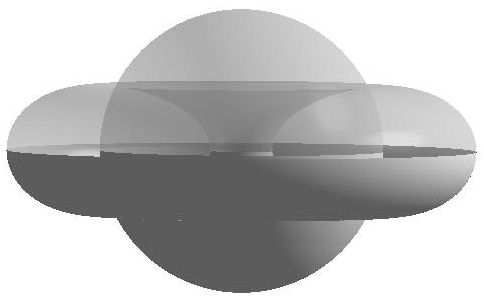
Figure 1. The closed, embedded self-similar ”toruspheres” Σg23superscriptsubscriptΣ𝑔2superscript3\Sigma_{g}^{2}\subseteq\mathbb{R}^{3} of genus g𝑔g in Theorem 1. Showing: Immersed singular configuration, before handle insertion along two intersection curves (drawn with MATLAB).

The Neumann version (N1’) of the non-degeneracy conditions will be used for the construction of the closed, embedded self-shrinkers where one solves the self-shrinker equations for graphs with the Neumann conditions over the circle of intersection of the torus and symmetry plane 𝕋2𝒫superscript𝕋2𝒫\mathbb{T}^{2}\cap\mathcal{P}, where 𝕋2superscript𝕋2\mathbb{T}^{2} denotes a self-shrinking torus. Then the closed surfaces are obtained via simple doubling, by reflection through this plane, where standard regularity theory guarantees smoothness.

Yet another important version of the above conditions, is the one obtained by imposing symmetries, say under a large (discrete) subgroup GO(3)𝐺𝑂3G\subseteq O(3), throughout the construction. Indeed, one may then restrict to verifying the non-degeneracy conditions (N1)–(N2) under the additional assumption of the symmetries in G𝐺G.

While some properties of the Jacobi fields can be deduced from the known eigenvalues and eigenfunctions for the stability operator \mathcal{L} (see e.g. [CM2]), one does not seem to obtain enough accurate information for our purposes. We show how to estimate the quantities using the (generalized) Bellman-Grönwall’s inequalities for second order Sturm-Liouville problems, and explicit test functions.

The care one needs to exercise when estimating the explicit constants, as well as the number and complexity of the barriers and test functions one needs to choose, becomes significant owing to mainly two factors: 1) The large Lipschitz constants of the PDE system (relative to the scale of the self-shrinking torus). The geometric reason that this happens is that the Gauß curvature in the metric on Angenent’s upper half-plane has a maximal value of around 30 along the candidate torus (with the maximum occurring at the point nearest to the origin in 3superscript3\mathbb{R}^{3}), giving naive characteristic conjugate distances of down to πK0.5similar-to𝜋𝐾0.5\frac{\pi}{\sqrt{K}}\sim 0.5, while the circumference of the torus is around 7similar-toabsent7\sim 7, in the metric. Hence the solutions to Jacobi’s equation can be expected to, and indeed do, oscillate several times around the circumference of 𝕋2superscript𝕋2\mathbb{T}^{2}, in a non-uniform way and yet just fall short of ”matching up” smoothly. Furthermore: 2) The location of the conjugate points on 𝕊2superscript𝕊2\mathbb{S}^{2} for the appropriate Jacobi equation is very near the singular curve 𝒞¯¯𝒞\underline{\mathcal{C}} (i.e. the boundaries of the connected components of 𝒞¯¯𝒞\mathcal{M}\setminus\underline{\mathcal{C}}), which also requires tighter estimates.

Hence it takes work to strengthen the estimates to a useful form. One device to do this is what could be called the ”sesqui”-shooting problem in Definition 2.4, for identifying the position of the torus, where ”sesqui” refers to the fact that it is a double shooting problem but with a compatibility condition linking the two: That each pair of curves always meet at a simple, explicitly known solution. Here we take the round cylinder of radius 22\sqrt{2} as reference. Since the errors are exponential in the integral of the Lipschitz constants, one may by virtue of the sesqui-shooting roughly take the square-root of the errors, which allows us to obtain bounds with explicit constants of the order of 101superscript10110^{1}102superscript10210^{2} instead of 104superscript10410^{4}.

Although reduced in volume by the above discussion, it turns out that the explicit choice of test functions (f.ex. adequate piecewise polynomial choices can easily be found using a Taylor expansion fit at selected points, deduced from a numerical solution to the PDEs), to insert into the key estimates in Section 2, still take up several pages, and is not in itself very enlightening material to include. The computational job of checking the estimates for the many low-degree polynomials is in any case best carried out using computer software. The corresponding figures throughout this paper, showing Angenent’s torus and the relevant Jacobi fields, were likewise computed and drawn in MATLAB.

Thus, the present paper does not contain the most efficient result that one could hope for, by amounting in effect to the reduction of the rigorous proof of the existence of closed self-shrinkers with genus to the still non-trivial algorithmic task of finding the zeros of several explicit low-order polynomials with integer coefficients (of course a task a computer easily manages rigorously).

2. ε𝜀\varepsilon-Geodesics, δ𝛿\delta-Jacobi Fields: A Quantitative Self-Shrinking Torus 𝕋2superscript𝕋2\mathbb{T}^{2}

2.1. Existence of 𝕋2superscript𝕋2\mathbb{T}^{2}, With Geometric Estimates

In order to later understand precisely the kernel of the stability operators, we need to establish a detailed quantitative version of the existence of Angenent’s torus. Towards the end of this section we will arrive at the basic, explicit estimates on the location and geometric quantities of such a torus, but we will first work out the explicit estimates for also the Jacobi equation before finalizing the choices in the estimate, in order to require as little as possible of the test functions.
Refer to caption
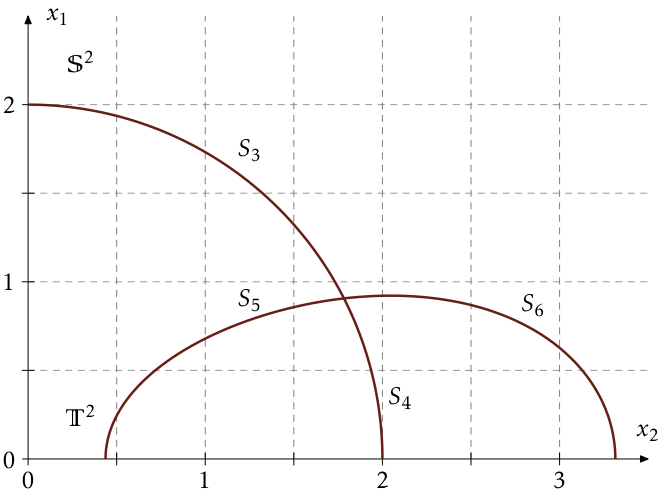
Figure 2. The connected components of 𝒲^=(𝕊2𝕋2)(𝕊2𝕋2)^𝒲superscript𝕊2superscript𝕋2superscript𝕊2superscript𝕋2\hat{\mathcal{W}}=(\mathbb{S}^{2}\cup\mathbb{T}^{2})\setminus(\mathbb{S}^{2}\cap\mathbb{T}^{2}). The self-intersecting initial surface is generated by rotation around the x1subscript𝑥1x_{1}-axis and reflection in the x2subscript𝑥2x_{2}-axis.

We note that much less complicated estimates (and ditto test functions) would ensure the mere existence, leading to a different proof of the self-shrinking ”doughnut” existence result from [An92], in the 333-dimensional case. But as explained, here we will need very precise estimates of several aspects of the geometry of 𝕋2superscript𝕋2\mathbb{T}^{2}.

Proposition 2.1.

Let εgap=103subscript𝜀gapsuperscript103\varepsilon_{\textrm{gap}}=10^{-3}. There exists a closed, embedded, self-shrinking torus of revolution 𝕋2superscript𝕋2\mathbb{T}^{2} with the following properties:

  • (1)

    The torus is (x1x1maps-tosubscript𝑥1subscript𝑥1x_{1}\mapsto-x_{1})-symmetric.

  • (2)

    𝕋2superscript𝕋2\mathbb{T}^{2} intersects the x2subscript𝑥2x_{2}-axis orthogonally at two heights a+>a>0superscript𝑎superscript𝑎0a^{+}>a^{-}>0,

    (2.1) 4034121752εgapmatrix40341217matrix52subscript𝜀gap\displaystyle\begin{matrix}\frac{4034}{1217}\end{matrix}-\begin{matrix}\frac{5}{2}\end{matrix}\varepsilon_{\textrm{gap}} <a+<40341217+52εgap,absentsuperscript𝑎matrix40341217matrix52subscript𝜀gap\displaystyle<a^{+}<\begin{matrix}\frac{4034}{1217}\end{matrix}+\begin{matrix}\frac{5}{2}\end{matrix}\varepsilon_{\textrm{gap}},
    (2.2) 716398matrix716matrix398\displaystyle\begin{matrix}\frac{7}{16}\end{matrix}-\begin{matrix}\frac{3}{98}\end{matrix} <a<716+398.absentsuperscript𝑎matrix716matrix398\displaystyle<a^{-}<\begin{matrix}\frac{7}{16}\end{matrix}+\begin{matrix}\frac{3}{98}\end{matrix}.
  • (3)

    𝕋2superscript𝕋2\mathbb{T}^{2} intersects the sphere 𝕊2superscript𝕊2\mathbb{S}^{2} of radius 2 at two points p±=(±x𝕊2,y𝕊2)superscript𝑝plus-or-minusplus-or-minussubscript𝑥superscript𝕊2subscript𝑦superscript𝕊2p^{\pm}=(\pm x_{\mathbb{S}^{2}},y_{\mathbb{S}^{2}}), where:

    (2.3) p±(±2932,4123)25εgap.subscriptnormsuperscript𝑝plus-or-minusplus-or-minusmatrix2932matrix4123superscript25subscript𝜀gap\displaystyle\left\|p^{\pm}-\left(\pm\begin{matrix}\frac{29}{32}\end{matrix},\begin{matrix}\frac{41}{23}\end{matrix}\right)\right\|_{\mathbb{R}^{2}}\leq 5\varepsilon_{\textrm{gap}}.

    Correspondingly, the angles (±e1,p±)plus-or-minussubscript𝑒1superscript𝑝plus-or-minus\angle(\pm\vec{e}_{1},p^{\pm}) from the x1subscript𝑥1x_{1}-axis satisfy:

    (2.4) |(±e1,p±)1110|120.plus-or-minussubscript𝑒1superscript𝑝plus-or-minusmatrix1110matrix120\big{|}\angle(\pm\vec{e}_{1},p^{\pm})-\begin{matrix}\frac{11}{10}\end{matrix}\big{|}\leq\begin{matrix}\frac{1}{20}\end{matrix}.
Remark 2.2.

Note that there is no assertion or proof of uniqueness of 𝕋2superscript𝕋2\mathbb{T}^{2} with these properties, although this is expected to be true.

Proof.

We first need to describe the double shooting problem (or rather ”sesqui”-shooting problem, since we remove one parameter). For this we need an elementary lemma, which can either be proved (in a weaker version) using the approximation methods described later in this section, or by analysis directly of the ODE in (2.32).

Lemma 2.3.

For each d[0,2]𝑑02d\in[0,\sqrt{2}] let γd:[0,)+×:subscript𝛾𝑑0superscript\gamma_{d}:[0,\infty)\to\mathbb{R}^{+}\times\mathbb{R} be the geodesic starting at (0,d)0𝑑(0,d) with initial derivative γd(0)=(1,0)superscriptsubscript𝛾𝑑010\gamma_{d}^{\prime}(0)=(1,0) and consider the first time t0(d)superscript𝑡0𝑑t^{0}(d) such that γdsubscript𝛾𝑑\gamma_{d} intersects the cylinder geodesic {x2=2}subscript𝑥22\{x_{2}=\sqrt{2}\}. Then the function I:[0,2][0,2]:𝐼0202I:[0,\sqrt{2}]\to[0,\sqrt{2}] given by

I(d):=x1(γs(t0(d))),assign𝐼𝑑subscript𝑥1subscript𝛾𝑠superscript𝑡0𝑑I(d):=x_{1}(\gamma_{s}(t^{0}(d))),

is continuous and strictly increasing. It satisfies the bounds:

1supd[1332,1532]I(d)54.1subscriptsupremum𝑑matrix1332matrix1532superscript𝐼𝑑541\leq\sup_{d\in[\begin{matrix}\frac{13}{32}\end{matrix},\begin{matrix}\frac{15}{32}\end{matrix}]}I^{\prime}(d)\leq\frac{5}{4}.
Definition 2.4 (”Sesqui”-Shooting Problem).
  • (i)

    Fix a>2𝑎2a>\sqrt{2}.

  • (ii)

    Let γa:[0,ta]+×:subscript𝛾𝑎0subscript𝑡𝑎superscript\gamma_{a}:[0,t_{a}]\to\mathbb{R}^{+}\times\mathbb{R} be the fully extended geodesic contained in {x10}subscript𝑥10\{x_{1}\geq 0\}, with initial conditions γa(0)=(0,a)subscript𝛾𝑎00𝑎\gamma_{a}(0)=(0,a) and γa(0)=(1,0)superscriptsubscript𝛾𝑎010\gamma_{a}^{\prime}(0)=(1,0).

  • (iii)

    By the maximum principle for (2.32), we have γa{x2=2}subscript𝛾𝑎subscript𝑥22\gamma_{a}\cap\{x_{2}=\sqrt{2}\}\neq\emptyset. Assume that the first point of γasubscript𝛾𝑎\gamma_{a} crossing 22\sqrt{2} belongs to {0<x12}0subscript𝑥12\{0<x_{1}\leq\sqrt{2}\}, and denote the time it happens by t0(a)superscript𝑡0𝑎t^{0}(a).

  • (iv)

    By the preceding Lemma, there exists a unique b(a)[0,2]𝑏𝑎02b(a)\in[0,\sqrt{2}] and s0(a)superscript𝑠0𝑎s^{0}(a) such that for γbsubscript𝛾𝑏\gamma_{b} on [0,s0]0superscript𝑠0[0,s^{0}] with γb(0)=(0,b)subscript𝛾𝑏00𝑏\gamma_{b}(0)=(0,b) and γb(0)=(1,0)superscriptsubscript𝛾𝑏010\gamma_{b}^{\prime}(0)=(1,0), we have

    γa(t0(a))=γb(s0(a)).subscript𝛾𝑎superscript𝑡0𝑎subscript𝛾𝑏superscript𝑠0𝑎\gamma_{a}(t^{0}(a))=\gamma_{b}(s^{0}(a)).
  • (iv)

    Define Φ(a)Φ𝑎\Phi(a) by

    Φ(a):=e3(γa(t0(a))×γb(s0(a))|γa(t0(a))||γb(s0(a))|,\Phi(a):=\frac{\vec{e_{3}}\cdot(\gamma^{\prime}_{a}(t^{0}(a))\times\gamma^{\prime}_{b}(s^{0}(a))}{|\gamma^{\prime}_{a}(t^{0}(a))||\gamma^{\prime}_{b}(s^{0}(a))|},

    or equivalently the oriented angle between the tangents of γasubscript𝛾𝑎\gamma_{a} and γbsubscript𝛾𝑏\gamma_{b} at the intersection point.

The following lemma is clear from the definition:

Lemma 2.5.

The function ΦΦ\Phi in Definition 2.4 is well-defined and continuous, on the open connected set of values a>2𝑎2a>\sqrt{2} with the property that the first point of intersection of γasubscript𝛾𝑎\gamma_{a} with {x2=2}subscript𝑥22\{x_{2}=\sqrt{2}\} belongs to {x1(0,2)}subscript𝑥102\{x_{1}\in(0,\sqrt{2})\}.

The strategy for the proof of the proposition will now be to prove for two different nearby pairs (a+,b+)superscript𝑎superscript𝑏(a^{+},b^{+}) and (a,b)superscript𝑎superscript𝑏(a^{-},b^{-}), that will be chosen such that they are geodesics broken at the cylinder {x2=2}subscript𝑥22\{x_{2}=\sqrt{2}\}, that:

(2.5) Φ(a+)>0,Φsuperscript𝑎0\displaystyle\Phi(a^{+})>0,
(2.6) Φ(a)<0.Φsuperscript𝑎0\displaystyle\Phi(a^{-})<0.

Existence then follows, from the intermediate value theorem, of a pair (a0,b0)superscript𝑎0superscript𝑏0(a^{0},b^{0}) such that:

(2.7) Φ(a0)=0,Φsuperscript𝑎00\displaystyle\Phi(a^{0})=0,
(2.8) a<a0<a+,superscript𝑎superscript𝑎0superscript𝑎\displaystyle a^{-}<a^{0}<a^{+},
(2.9) b<b0<b+.superscript𝑏superscript𝑏0superscript𝑏\displaystyle b^{-}<b^{0}<b^{+}.

The estimates leading to the proof of (2.5)–(2.6) will then lead to the estimates in the proposition.

Consider now a curve (parametrized by any parameter t𝑡t),

γ(t)=(x(t),y(t)).𝛾𝑡𝑥𝑡𝑦𝑡\gamma(t)=(x(t),y(t)).

Then the equation for γ𝛾\gamma to generate a self-shrinker by rotation reads:

x′′yy′′x=[yxxy2xy]((x)2+(y)2).superscript𝑥′′superscript𝑦superscript𝑦′′superscript𝑥delimited-[]𝑦superscript𝑥𝑥superscript𝑦2superscript𝑥𝑦superscriptsuperscript𝑥2superscriptsuperscript𝑦2x^{\prime\prime}y^{\prime}-y^{\prime\prime}x^{\prime}=\left[\frac{yx^{\prime}-xy^{\prime}}{2}-\frac{x^{\prime}}{y}\right]\left((x^{\prime})^{2}+(y^{\prime})^{2}\right).

We need the following simple lemma:

Lemma 2.6.

If we define the operator 1subscript1\mathcal{M}_{1} acting on C2superscript𝐶2C^{2}-functions u:I:𝑢𝐼u:I\to\mathbb{R}, for some interval I[0,]𝐼0I\subseteq[0,\infty], by

(2.10) 1(u,p):=[x1pu2+1u](1+p2),assignsubscript1𝑢𝑝delimited-[]subscript𝑥1𝑝𝑢21𝑢1superscript𝑝2\mathcal{M}_{1}(u,p):=\Big{[}\frac{x_{1}p-u}{2}+\frac{1}{u}\Big{]}\big{(}1+p^{2}\big{)},

then the function u(x1)𝑢subscript𝑥1u(x_{1}), a graph over the x1subscript𝑥1x_{1}-axis, generates a self-shrinker by rotation (around x1subscript𝑥1x_{1}) if and only if

(2.11) u′′=1(u,u).superscript𝑢′′subscript1𝑢superscript𝑢u^{\prime\prime}=\mathcal{M}_{1}(u,u^{\prime}).

Likewise for graphs over the x2subscript𝑥2x_{2}-axis, defining

(2.12) 2(f,q):=[(x221x2)qf2](1+q2),assignsubscript2𝑓𝑞delimited-[]subscript𝑥221subscript𝑥2𝑞𝑓21superscript𝑞2\mathcal{M}_{2}(f,q):=\left[\left(\frac{x_{2}}{2}-\frac{1}{x_{2}}\right)q-\frac{f}{2}\right]\left(1+q^{2}\right),

again characterizes such solutions via

(2.13) f′′=2(f,f).superscript𝑓′′subscript2𝑓superscript𝑓f^{\prime\prime}=\mathcal{M}_{2}(f,f^{\prime}).

The lemma is shown directly from the definition of a self-shrinker (see [KMø]). We now compute that:

(2.14) u1(u,p)=[121u2](1+p2),𝑢subscript1𝑢𝑝delimited-[]121superscript𝑢21superscript𝑝2\displaystyle\frac{\partial}{\partial u}\mathcal{M}_{1}(u,p)=\left[-\frac{1}{2}-\frac{1}{u^{2}}\right](1+p^{2}),
(2.15) p1(u,p)=x12(1+p2)+2p[x1pu2+1u],𝑝subscript1𝑢𝑝subscript𝑥121superscript𝑝22𝑝delimited-[]subscript𝑥1𝑝𝑢21𝑢\displaystyle\frac{\partial}{\partial p}\mathcal{M}_{1}(u,p)=\frac{x_{1}}{2}(1+p^{2})+2p\left[\frac{x_{1}p-u}{2}+\frac{1}{u}\right],
(2.16) f2(f,q)=12(1+q2),𝑓subscript2𝑓𝑞121superscript𝑞2\displaystyle\frac{\partial}{\partial f}\mathcal{M}_{2}(f,q)=-\frac{1}{2}\left(1+q^{2}\right),
(2.17) q2(f,q)=(x221x2)(1+3q2)fq.𝑞subscript2𝑓𝑞subscript𝑥221subscript𝑥213superscript𝑞2𝑓𝑞\displaystyle\frac{\partial}{\partial q}\mathcal{M}_{2}(f,q)=\left(\frac{x_{2}}{2}-\frac{1}{x_{2}}\right)(1+3q^{2})-fq.

We will first consider graphs u:[0,35]:𝑢0matrix35u:[0,\begin{matrix}\frac{3}{5}\end{matrix}]\to\mathbb{R}. Now, considering an approximate solution U𝑈U, fix the quantity ε1Tsuperscriptsubscript𝜀1𝑇\varepsilon_{1}^{T}, later to be chosen, which reflects the order of magnitude of the precision with which we wish to determine the position of 𝕋2superscript𝕋2\mathbb{T}^{2} on this interval.

(2.18) 1(U,U)1(u,u)=(Uu)u1(ξ,u)+(Uu)p1(U,ξ),subscript1𝑈superscript𝑈subscript1𝑢superscript𝑢𝑈𝑢𝑢subscript1𝜉superscript𝑢superscript𝑈superscript𝑢𝑝subscript1𝑈superscript𝜉\mathcal{M}_{1}(U,U^{\prime})-\mathcal{M}_{1}(u,u^{\prime})=(U-u)\frac{\partial}{\partial u}\mathcal{M}_{1}(\xi,u^{\prime})+(U^{\prime}-u^{\prime})\frac{\partial}{\partial p}\mathcal{M}_{1}(U,\xi^{\prime}),

for some ξ[U(x1),u(x1)]𝜉𝑈subscript𝑥1𝑢subscript𝑥1\xi\in[U(x_{1}),u(x_{1})] and ξ[U(x1),u(x1)]superscript𝜉superscript𝑈subscript𝑥1superscript𝑢subscript𝑥1\xi^{\prime}\in[U^{\prime}(x_{1}),u^{\prime}(x_{1})].

Top of the torus: x1subscript𝑥1x_{1}-graph

Assume we have the uniform estimates:

|U′′1(U,U)|ε1T,superscript𝑈′′subscript1𝑈superscript𝑈superscriptsubscript𝜀1𝑇|U^{\prime\prime}-\mathcal{M}_{1}(U,U^{\prime})|\leq\varepsilon_{1}^{T},

for some ε1Tsuperscriptsubscript𝜀1𝑇\varepsilon_{1}^{T}. Assume also the following bounds:

0x1|12+1ξ2|(1+(u(x1))2)𝑑x145x1,x1[0,35],|ξU(x1)|ε0,formulae-sequencesuperscriptsubscript0subscript𝑥1121superscript𝜉21superscriptsuperscript𝑢subscript𝑥12differential-dsubscript𝑥145subscript𝑥1formulae-sequencesubscript𝑥10matrix35𝜉𝑈subscript𝑥1subscript𝜀0\displaystyle\int_{0}^{x_{1}}\left|\frac{1}{2}+\frac{1}{\xi^{2}}\right|(1+(u^{\prime}(x_{1}))^{2})dx_{1}\leq\frac{4}{5}x_{1},\quad x_{1}\in[0,\begin{matrix}\frac{3}{5}\end{matrix}],\quad|\xi-U(x_{1})|\leq\varepsilon_{0},
0x1|x12(1+(ξ)2)+2ξ[x1ξU(x1)2+1U(x1)]|𝑑x183x12,x1[0,35],|ξU(x1)|ε0.formulae-sequencesuperscriptsubscript0subscript𝑥1subscript𝑥121superscriptsuperscript𝜉22superscript𝜉delimited-[]subscript𝑥1superscript𝜉𝑈subscript𝑥121𝑈subscript𝑥1differential-dsubscript𝑥183superscriptsubscript𝑥12formulae-sequencesubscript𝑥10matrix35superscript𝜉superscript𝑈subscript𝑥1subscript𝜀0\displaystyle\int_{0}^{x_{1}}\left|\frac{x_{1}}{2}(1+(\xi^{\prime})^{2})+2\xi^{\prime}\left[\frac{x_{1}\xi^{\prime}-U(x_{1})}{2}+\frac{1}{U(x_{1})}\right]\right|dx_{1}\leq\frac{8}{3}x_{1}^{2},\quad x_{1}\in[0,\begin{matrix}\frac{3}{5}\end{matrix}],\quad|\xi^{\prime}-U^{\prime}(x_{1})|\leq\varepsilon_{0}.

If we let φ(x1):=|U(x1)u(x1)|assign𝜑subscript𝑥1superscript𝑈subscript𝑥1superscript𝑢subscript𝑥1\varphi(x_{1}):=|U^{\prime}(x_{1})-u^{\prime}(x_{1})|, we can now estimate (recall that one has ||f||=|f′′|superscriptsuperscript𝑓superscript𝑓′′||f^{\prime}|^{\prime}|=|f^{\prime\prime}| almost everywhere):

(2.19) φ(x1)||Uu||=a.e|U′′u′′||1(U,U)1(u,u)|+ε1T|u1(ξ,u)||Uu|+|p1(U,ξ)||Uu|+ε1T|p1(U,ξ)|φ(x1)+|u1(ξ,u)|0x1φ(s)𝑑s+|u1(ξ,u)||U(0)u(0)|+ε1T.superscript𝜑subscript𝑥1superscriptsuperscript𝑈superscript𝑢a.esuperscript𝑈′′superscript𝑢′′subscript1𝑈superscript𝑈subscript1𝑢superscript𝑢superscriptsubscript𝜀1𝑇subscript𝑢subscript1𝜉superscript𝑢𝑈𝑢subscript𝑝subscript1𝑈superscript𝜉superscript𝑈superscript𝑢superscriptsubscript𝜀1𝑇subscript𝑝subscript1𝑈superscript𝜉limit-from𝜑subscript𝑥1subscript𝑢subscript1𝜉superscript𝑢limit-fromsuperscriptsubscript0subscript𝑥1𝜑𝑠differential-d𝑠subscript𝑢subscript1𝜉superscript𝑢𝑈0𝑢0superscriptsubscript𝜀1𝑇\begin{split}\varphi^{\prime}(x_{1})&\leq\left||U^{\prime}-u^{\prime}|^{\prime}\right|\overset{\textrm{a.e}}{=}|U^{\prime\prime}-u^{\prime\prime}|\\ &\leq|\mathcal{M}_{1}(U,U^{\prime})-\mathcal{M}_{1}(u,u^{\prime})|+\varepsilon_{1}^{T}\\ &\leq|\partial_{u}\mathcal{M}_{1}(\xi,u^{\prime})||U-u|+|\partial_{p}\mathcal{M}_{1}(U,\xi^{\prime})||U^{\prime}-u^{\prime}|+\varepsilon_{1}^{T}\\ &\leq|\partial_{p}\mathcal{M}_{1}(U,\xi^{\prime})|\varphi(x_{1})+|\partial_{u}\mathcal{M}_{1}(\xi,u^{\prime})|\int_{0}^{x_{1}}\varphi(s)ds+|\partial_{u}\mathcal{M}_{1}(\xi,u^{\prime})||U(0)-u(0)|+\varepsilon_{1}^{T}.\end{split}

Thus we integrate this inequality, which holds almost everywhere with respect to the Lebesgue measure, and get:

φ(x1)𝜑subscript𝑥1\displaystyle\varphi(x_{1}) φ(0)+0x1|p1(U,ξ)(s)|φ(s)𝑑s+0x1|u1(ξ,u)(t)|0tφ(s)𝑑s𝑑tabsent𝜑0superscriptsubscript0subscript𝑥1subscript𝑝subscript1𝑈superscript𝜉𝑠𝜑𝑠differential-d𝑠superscriptsubscript0subscript𝑥1subscript𝑢subscript1𝜉superscript𝑢𝑡superscriptsubscript0𝑡𝜑𝑠differential-d𝑠differential-d𝑡\displaystyle\leq\varphi(0)+\int_{0}^{x_{1}}|\partial_{p}\mathcal{M}_{1}(U,\xi^{\prime})(s)|\varphi(s)ds+\int_{0}^{x_{1}}|\partial_{u}\mathcal{M}_{1}(\xi,u^{\prime})(t)|\int_{0}^{t}\varphi(s)dsdt
+45x1|U(0)u(0)|+ε1Tx1matrix45subscript𝑥1𝑈0𝑢0superscriptsubscript𝜀1𝑇subscript𝑥1\displaystyle\quad\quad\quad+\begin{matrix}\frac{4}{5}\end{matrix}x_{1}|U(0)-u(0)|+\varepsilon_{1}^{T}x_{1}
φ(0)+45x1|U(0)u(0)|+ε1Tx1+0x1[|p1(U,ξ)(s)|+45x1]φ(s)𝑑s.absent𝜑0matrix45subscript𝑥1𝑈0𝑢0superscriptsubscript𝜀1𝑇subscript𝑥1superscriptsubscript0subscript𝑥1delimited-[]subscript𝑝subscript1𝑈superscript𝜉𝑠matrix45subscript𝑥1𝜑𝑠differential-d𝑠\displaystyle\leq\varphi(0)+\begin{matrix}\frac{4}{5}\end{matrix}x_{1}|U(0)-u(0)|+\varepsilon_{1}^{T}x_{1}+\int_{0}^{x_{1}}\Big{[}|\partial_{p}\mathcal{M}_{1}(U,\xi^{\prime})(s)|+\begin{matrix}\frac{4}{5}\end{matrix}x_{1}\Big{]}\varphi(s)ds.

We are now ready to use the integral form of Grönwall-Bellman’s inequality, namely for α(t)𝛼𝑡\alpha(t) a non-decreasing function:

tI:φ(t)α(t)+atβ(s)φ(s)𝑑stI:φ(t)α(t)exp{atβ(s)𝑑s}.:for-all𝑡𝐼formulae-sequence𝜑𝑡𝛼𝑡superscriptsubscript𝑎𝑡𝛽𝑠𝜑𝑠differential-d𝑠for-all𝑡𝐼:𝜑𝑡𝛼𝑡superscriptsubscript𝑎𝑡𝛽𝑠differential-d𝑠\forall t\in I:\varphi(t)\leq\alpha(t)+\int_{a}^{t}\beta(s)\varphi(s)ds\quad\Longrightarrow\quad\forall t\in I:\varphi(t)\leq\alpha(t)\exp\left\{\int_{a}^{t}\beta(s)ds\right\}.

Here we thus conclude from the above, that

(2.20) φ(x1)[φ(0)+45x1|U(0)u(0)|+ε1Tx1]exp{83x12+45x12},𝜑subscript𝑥1delimited-[]𝜑0matrix45subscript𝑥1𝑈0𝑢0superscriptsubscript𝜀1𝑇subscript𝑥1matrix83superscriptsubscript𝑥12matrix45superscriptsubscript𝑥12\varphi(x_{1})\leq\Big{[}\varphi(0)+\begin{matrix}\frac{4}{5}\end{matrix}x_{1}|U(0)-u(0)|+\varepsilon_{1}^{T}x_{1}\Big{]}\exp\Big{\{}\begin{matrix}\frac{8}{3}\end{matrix}x_{1}^{2}+\begin{matrix}\frac{4}{5}\end{matrix}x_{1}^{2}\Big{\}},

so that here we obtain the estimates (for φ(0)=0𝜑00\varphi(0)=0):

|U(x1)u(x1)|superscript𝑈subscript𝑥1superscript𝑢subscript𝑥1\displaystyle|U^{\prime}(x_{1})-u^{\prime}(x_{1})| 35exp(156125)(ε1T+45|U(0)u(0)|),absentmatrix35matrix156125superscriptsubscript𝜀1𝑇matrix45𝑈0𝑢0\displaystyle\leq\begin{matrix}\frac{3}{5}\end{matrix}\exp(\begin{matrix}\frac{156}{125}\end{matrix})(\varepsilon_{1}^{T}+\begin{matrix}\frac{4}{5}\end{matrix}|U(0)-u(0)|),
|U(x1)u(x1)|𝑈subscript𝑥1𝑢subscript𝑥1\displaystyle|U(x_{1})-u(x_{1})| |U(0)u(0)|+(ε1T+45|U(0)u(0)|)035sexp(5215s2)𝑑sabsent𝑈0𝑢0superscriptsubscript𝜀1𝑇matrix45𝑈0𝑢0superscriptsubscript0matrix35𝑠matrix5215superscript𝑠2differential-d𝑠\displaystyle\leq|U(0)-u(0)|+(\varepsilon_{1}^{T}+\begin{matrix}\frac{4}{5}\end{matrix}|U(0)-u(0)|)\int_{0}^{\begin{matrix}\frac{3}{5}\end{matrix}}s\exp\big{(}\begin{matrix}\frac{52}{15}\end{matrix}s^{2}\big{)}ds
=|U(0)u(0)|+15104(exp(5215(35)2)1)(ε1T+45|U(0)u(0)|)absent𝑈0𝑢0matrix15104matrix5215superscriptmatrix3521superscriptsubscript𝜀1𝑇matrix45𝑈0𝑢0\displaystyle=|U(0)-u(0)|+\begin{matrix}\frac{15}{104}\end{matrix}\big{(}\exp\big{(}\begin{matrix}\frac{52}{15}\end{matrix}(\begin{matrix}\frac{3}{5}\end{matrix})^{2}\big{)}-1\big{)}(\varepsilon_{1}^{T}+\begin{matrix}\frac{4}{5}\end{matrix}|U(0)-u(0)|)
2380|U(0)u(0)|+925ε1T.absentmatrix2380𝑈0𝑢0matrix925superscriptsubscript𝜀1𝑇\displaystyle\leq\begin{matrix}\frac{23}{80}\end{matrix}|U(0)-u(0)|+\begin{matrix}\frac{9}{25}\end{matrix}\varepsilon_{1}^{T}.

Top of the torus: x2subscript𝑥2x_{2}-graph to the sphere

We continue with the next part, which is graphical over the x2subscript𝑥2x_{2}-axis. In this region we again let ψ(x2):=|Ff|assign𝜓subscript𝑥2superscript𝐹superscript𝑓\psi(x_{2}):=|F^{\prime}-f^{\prime}|. Here we will assume the estimate

(2.21) |F′′2(F,F)|ε2T,superscript𝐹′′subscript2𝐹superscript𝐹superscriptsubscript𝜀2𝑇|F^{\prime\prime}-\mathcal{M}_{2}(F,F^{\prime})|\leq\varepsilon_{2}^{T},

and furthermore the estimates on x2[y𝕊2,uT(3/5)]subscript𝑥2subscript𝑦superscript𝕊2subscript𝑢𝑇35x_{2}\in[y_{\mathbb{S}^{2}},u_{T}(3/5)]

Iu(2)=x2uT(3/5)|12(1+(F)2)|𝑑x2138x22,subscriptsuperscript𝐼2𝑢superscriptsubscriptsubscript𝑥2subscript𝑢𝑇35121superscriptsuperscript𝐹2differential-dsubscript𝑥2matrix138matrixsubscript𝑥22\displaystyle I^{(2)}_{u}=\int_{x_{2}}^{u_{T}(3/5)}\left|\frac{1}{2}(1+(F^{\prime})^{2})\right|dx_{2}\leq\begin{matrix}\frac{13}{8}\end{matrix}-\begin{matrix}\frac{x_{2}}{2}\end{matrix},
Ip(2)=x2uT(3/5)|(x221x2)(1+3(ξ)2)F(x2)ξ|𝑑x274910(x2y𝕊2)2.subscriptsuperscript𝐼2𝑝superscriptsubscriptsubscript𝑥2subscript𝑢𝑇35subscript𝑥221subscript𝑥213superscriptsuperscript𝜉2𝐹subscript𝑥2superscript𝜉differential-dsubscript𝑥2matrix74matrix910superscriptsubscript𝑥2subscript𝑦superscript𝕊22\displaystyle I^{(2)}_{p}=\int_{x_{2}}^{u_{T}(3/5)}\left|\left(\frac{x_{2}}{2}-\frac{1}{x_{2}}\right)(1+3(\xi^{\prime})^{2})-F(x_{2})\xi^{\prime}\right|dx_{2}\leq\begin{matrix}\frac{7}{4}\end{matrix}-\begin{matrix}\frac{9}{10}\end{matrix}\left(x_{2}-y_{\mathbb{S}^{2}}\right)^{2}.

We can then estimate as follows:

ψ(x2)superscript𝜓subscript𝑥2\displaystyle\psi^{\prime}(x_{2}) |u2||Ff|+|p2||Ff|+ε2Tabsentsubscript𝑢subscript2𝐹𝑓subscript𝑝subscript2superscript𝐹superscript𝑓superscriptsubscript𝜀2𝑇\displaystyle\leq\left|\partial_{u}\mathcal{M}_{2}\right||F-f|+\left|\partial_{p}\mathcal{M}_{2}\right||F^{\prime}-f^{\prime}|+\varepsilon_{2}^{T}
|u2|x2aψ(s)𝑑s+|p2|ψ(x2)+|u2||F(a)f(a)|+ε2T,absentsubscript𝑢subscript2superscriptsubscriptsubscript𝑥2𝑎𝜓𝑠differential-d𝑠subscript𝑝subscript2𝜓subscript𝑥2subscript𝑢subscript2𝐹𝑎𝑓𝑎superscriptsubscript𝜀2𝑇\displaystyle\leq\left|\partial_{u}\mathcal{M}_{2}\right|\int_{x_{2}}^{a}\psi(s)ds+\left|\partial_{p}\mathcal{M}_{2}\right|\psi(x_{2})+\left|\partial_{u}\mathcal{M}_{2}\right||F(a)-f(a)|+\varepsilon_{2}^{T},

which integrates to

(2.22) ψ(x2)𝜓subscript𝑥2absent\displaystyle\psi(x_{2})\leq x2uT(3/5)[|p2|+138x22]ψ(s)𝑑s+(138x22)|F(uT(3/5))f(uT(3/5))|superscriptsubscriptsubscript𝑥2subscript𝑢𝑇35delimited-[]subscript𝑝subscript2matrix138matrixsubscript𝑥22𝜓𝑠differential-d𝑠matrix138matrixsubscript𝑥22𝐹subscript𝑢𝑇35𝑓subscript𝑢𝑇35\displaystyle\int_{x_{2}}^{u_{T}(3/5)}\left[|\partial_{p}\mathcal{M}_{2}|+\begin{matrix}\frac{13}{8}\end{matrix}-\begin{matrix}\frac{x_{2}}{2}\end{matrix}\right]\psi(s)ds+(\begin{matrix}\frac{13}{8}\end{matrix}-\begin{matrix}\frac{x_{2}}{2}\end{matrix})|F({u_{T}(3/5)})-f({u_{T}(3/5)})|
(2.23) +ε2T(uT(3/5)x2)+ψ(a),superscriptsubscript𝜀2𝑇subscript𝑢𝑇35subscript𝑥2𝜓𝑎\displaystyle\qquad+\varepsilon_{2}^{T}(u_{T}(3/5)-x_{2})+\psi(a),

so that, again by Grönwall-Bellman,

ψ(x2)𝜓subscript𝑥2absent\displaystyle\psi(x_{2})\leq [(138x22)|F(a)f(a)|+|F(a)f(a)|+ε2T(uT(3/5)x2)]×\displaystyle\Big{[}(\begin{matrix}\frac{13}{8}\end{matrix}-\begin{matrix}\frac{x_{2}}{2}\end{matrix})|F(a)-f(a)|+|F^{\prime}(a)-f^{\prime}(a)|+\varepsilon_{2}^{T}(u_{T}(3/5)-x_{2})\Big{]}\times
exp{74910(x2y𝕊2)2+(138x22)(uT(3/5)x2)}.matrix74matrix910superscriptsubscript𝑥2subscript𝑦superscript𝕊22matrix138matrixsubscript𝑥22subscript𝑢𝑇35subscript𝑥2\displaystyle\exp\left\{\begin{matrix}\frac{7}{4}\end{matrix}-\begin{matrix}\frac{9}{10}\end{matrix}\left(x_{2}-y_{\mathbb{S}^{2}}\right)^{2}+\left(\begin{matrix}\frac{13}{8}\end{matrix}-\begin{matrix}\frac{x_{2}}{2}\end{matrix}\right)\left(u_{T}(3/5)-x_{2}\right)\right\}.

The endpoint estimates for |F(x2)f(x2)|superscript𝐹subscript𝑥2superscript𝑓subscript𝑥2|F^{\prime}(x_{2})-f^{\prime}(x_{2})| are thus:

ψ(y𝕊2)𝜓subscript𝑦superscript𝕊2\displaystyle\psi(y_{\mathbb{S}^{2}}) 594|F(uT(3/5))f(uT(3/5))|+545|F(uT(3/5))f(uT(3/5))|+37720ε2Tabsentmatrix594𝐹subscript𝑢𝑇35𝑓subscript𝑢𝑇35matrix545superscript𝐹subscript𝑢𝑇35superscript𝑓subscript𝑢𝑇35matrix37720superscriptsubscript𝜀2𝑇\displaystyle\leq\begin{matrix}\frac{59}{4}\end{matrix}|F(u_{T}(3/5))-f(u_{T}(3/5))|+\begin{matrix}\frac{54}{5}\end{matrix}|F^{\prime}(u_{T}(3/5))-f^{\prime}(u_{T}(3/5))|+\begin{matrix}\frac{377}{20}\end{matrix}\varepsilon_{2}^{T}
594|U(F(uT(3/5)))u(f(uT(3/5)))||U(F(ξ))|+545|U(F(uT(3/5)))u(f(uT(3/5)))||U(F(uT(3/5)))||u(f(uT(3/5)))|+37720ε2Tabsentmatrix594𝑈𝐹subscript𝑢𝑇35𝑢𝑓subscript𝑢𝑇35superscript𝑈𝐹𝜉matrix545superscript𝑈𝐹subscript𝑢𝑇35superscript𝑢𝑓subscript𝑢𝑇35superscript𝑈𝐹subscript𝑢𝑇35superscript𝑢𝑓subscript𝑢𝑇35matrix37720superscriptsubscript𝜀2𝑇\displaystyle\leq\begin{matrix}\frac{59}{4}\end{matrix}\frac{|U(F(u_{T}(3/5)))-u(f(u_{T}(3/5)))|}{|U^{\prime}(F(\xi))|}+\begin{matrix}\frac{54}{5}\end{matrix}\frac{|U^{\prime}(F(u_{T}(3/5)))-u^{\prime}(f(u_{T}(3/5)))|}{|U^{\prime}(F(u_{T}(3/5)))||u^{\prime}(f(u_{T}(3/5)))|}+\begin{matrix}\frac{377}{20}\end{matrix}\varepsilon_{2}^{T}
5941011(925ε1T+2380|U(0)u(0)|)+545(1011)235exp(156125)(ε1T+45|U(0)u(0)|)+37720ε2Tabsentmatrix594matrix1011matrix925superscriptsubscript𝜀1𝑇matrix2380𝑈0𝑢0matrix545superscriptmatrix10112matrix35matrix156125superscriptsubscript𝜀1𝑇matrix45𝑈0𝑢0matrix37720superscriptsubscript𝜀2𝑇\displaystyle\leq\begin{matrix}\frac{59}{4}\end{matrix}\begin{matrix}\frac{10}{11}\end{matrix}\left(\begin{matrix}\frac{9}{25}\end{matrix}\varepsilon_{1}^{T}+\begin{matrix}\frac{23}{80}\end{matrix}|U(0)-u(0)|\right)+\begin{matrix}\frac{54}{5}\end{matrix}\left(\begin{matrix}\frac{10}{11}\end{matrix}\right)^{2}\begin{matrix}\frac{3}{5}\end{matrix}\exp(\begin{matrix}\frac{156}{125}\end{matrix})(\varepsilon_{1}^{T}+\begin{matrix}\frac{4}{5}\end{matrix}|U(0)-u(0)|)+\begin{matrix}\frac{377}{20}\end{matrix}\varepsilon_{2}^{T}
27|U(0)u(0)|+34ε1T+19ε2T.absent27𝑈0𝑢034superscriptsubscript𝜀1𝑇19superscriptsubscript𝜀2𝑇\displaystyle\leq 27|U(0)-u(0)|+34\varepsilon_{1}^{T}+19\varepsilon_{2}^{T}.

Integrating the above estimate for ψ(x2)𝜓subscript𝑥2\psi(x_{2}), we also get:

|F(y𝕊2)f(y𝕊2)|𝐹subscript𝑦superscript𝕊2𝑓subscript𝑦superscript𝕊2absent\displaystyle|F(y_{\mathbb{S}^{2}})-f(y_{\mathbb{S}^{2}})|\leq (1+638)|F(uT(3/5))f(uT(3/5))|+8320|F(uT(3/5))f(uT(3/5))|+13720ε2T1matrix638𝐹subscript𝑢𝑇35𝑓subscript𝑢𝑇35matrix8320superscript𝐹subscript𝑢𝑇35superscript𝑓subscript𝑢𝑇35matrix13720superscriptsubscript𝜀2𝑇\displaystyle(1+\begin{matrix}\frac{63}{8}\end{matrix})|F(u_{T}(3/5))-f(u_{T}(3/5))|+\begin{matrix}\frac{83}{20}\end{matrix}|F^{\prime}(u_{T}(3/5))-f^{\prime}(u_{T}(3/5))|+\begin{matrix}\frac{137}{20}\end{matrix}\varepsilon_{2}^{T}
\displaystyle\leq 12|U(0)u(0)|+15ε1T+7ε2T.12𝑈0𝑢015superscriptsubscript𝜀1𝑇7superscriptsubscript𝜀2𝑇\displaystyle 12|U(0)-u(0)|+15\varepsilon_{1}^{T}+7\varepsilon_{2}^{T}.

Top of the torus, x2subscript𝑥2x_{2}-graph from sphere to cylinder

We consider the region between the sphere and cylinder, and let again ψ(x2):=|Ff|assign𝜓subscript𝑥2superscript𝐹superscript𝑓\psi(x_{2}):=|F^{\prime}-f^{\prime}|. Here we will assume the estimate

(2.24) |F′′2(F,F)|ε3T,superscript𝐹′′subscript2𝐹superscript𝐹superscriptsubscript𝜀3𝑇|F^{\prime\prime}-\mathcal{M}_{2}(F,F^{\prime})|\leq\varepsilon_{3}^{T},

and furthermore the estimates on x2[y𝕊2,2]subscript𝑥2subscript𝑦superscript𝕊22x_{2}\in[y_{\mathbb{S}^{2}},\sqrt{2}]

Iu(2)=x2y𝕊2|12(1+(F)2)|𝑑x214(y𝕊2x2),subscriptsuperscript𝐼2𝑢superscriptsubscriptsubscript𝑥2subscript𝑦superscript𝕊2121superscriptsuperscript𝐹2differential-dsubscript𝑥2matrix14subscript𝑦superscript𝕊2subscript𝑥2\displaystyle I^{(2)}_{u}=\int_{x_{2}}^{y_{\mathbb{S}^{2}}}\left|\frac{1}{2}(1+(F^{\prime})^{2})\right|dx_{2}\leq\begin{matrix}\frac{1}{4}\end{matrix}(y_{\mathbb{S}^{2}}-x_{2}),
Ip(2)=x2y𝕊2|(x221x2)(1+3(ξ)2)F(x2)ξ|𝑑x22750(y𝕊2x2).subscriptsuperscript𝐼2𝑝superscriptsubscriptsubscript𝑥2subscript𝑦superscript𝕊2subscript𝑥221subscript𝑥213superscriptsuperscript𝜉2𝐹subscript𝑥2superscript𝜉differential-dsubscript𝑥2matrix2750subscript𝑦superscript𝕊2subscript𝑥2\displaystyle I^{(2)}_{p}=\int_{x_{2}}^{y_{\mathbb{S}^{2}}}\left|\left(\frac{x_{2}}{2}-\frac{1}{x_{2}}\right)(1+3(\xi^{\prime})^{2})-F(x_{2})\xi^{\prime}\right|dx_{2}\leq\begin{matrix}\frac{27}{50}\end{matrix}(y_{\mathbb{S}^{2}}-x_{2}).

We estimate as follows:

ψ(x2)superscript𝜓subscript𝑥2\displaystyle\psi^{\prime}(x_{2}) |u2||Ff|+|p2||Ff|+ε2Tabsentsubscript𝑢subscript2𝐹𝑓subscript𝑝subscript2superscript𝐹superscript𝑓superscriptsubscript𝜀2𝑇\displaystyle\leq\left|\partial_{u}\mathcal{M}_{2}\right||F-f|+\left|\partial_{p}\mathcal{M}_{2}\right||F^{\prime}-f^{\prime}|+\varepsilon_{2}^{T}
|u2|x2y𝕊2ψ(s)𝑑s+|p2|ψ(x2)+|u2||F(y𝕊2)f(y𝕊2)|+ε3T,absentsubscript𝑢subscript2superscriptsubscriptsubscript𝑥2subscript𝑦superscript𝕊2𝜓𝑠differential-d𝑠subscript𝑝subscript2𝜓subscript𝑥2subscript𝑢subscript2𝐹subscript𝑦superscript𝕊2𝑓subscript𝑦superscript𝕊2superscriptsubscript𝜀3𝑇\displaystyle\leq\left|\partial_{u}\mathcal{M}_{2}\right|\int_{x_{2}}^{y_{\mathbb{S}^{2}}}\psi(s)ds+\left|\partial_{p}\mathcal{M}_{2}\right|\psi(x_{2})+\left|\partial_{u}\mathcal{M}_{2}\right||F(y_{\mathbb{S}^{2}})-f(y_{\mathbb{S}^{2}})|+\varepsilon_{3}^{T},

which integrates to:

(2.25) ψ(x2)𝜓subscript𝑥2absent\displaystyle\psi(x_{2})\leq ψ(y𝕊2)+x2y𝕊2[|p2|+14(y𝕊2x2)]ψ(s)𝑑s+14(y𝕊2x2)|F(y𝕊2)f(y𝕊2)|+ε3T(y𝕊2x2),𝜓subscript𝑦superscript𝕊2superscriptsubscriptsubscript𝑥2subscript𝑦superscript𝕊2delimited-[]subscript𝑝subscript2matrix14subscript𝑦superscript𝕊2subscript𝑥2𝜓𝑠differential-d𝑠matrix14subscript𝑦superscript𝕊2subscript𝑥2𝐹subscript𝑦superscript𝕊2𝑓subscript𝑦superscript𝕊2superscriptsubscript𝜀3𝑇subscript𝑦superscript𝕊2subscript𝑥2\displaystyle\psi(y_{\mathbb{S}^{2}})+\int_{x_{2}}^{y_{\mathbb{S}^{2}}}\left[|\partial_{p}\mathcal{M}_{2}|+\begin{matrix}\frac{1}{4}\end{matrix}(y_{\mathbb{S}^{2}}-x_{2})\right]\psi(s)ds+\begin{matrix}\frac{1}{4}\end{matrix}(y_{\mathbb{S}^{2}}-x_{2})|F(y_{\mathbb{S}^{2}})-f(y_{\mathbb{S}^{2}})|+\varepsilon_{3}^{T}(y_{\mathbb{S}^{2}}-x_{2}),

so that, again by Grönwall-Bellman,

ψ(x2)𝜓subscript𝑥2absent\displaystyle\psi(x_{2})\leq [14(y𝕊2x2)|F(y𝕊2)f(y𝕊2)|+|F(y𝕊2)f(y𝕊2)|+ε3T(y𝕊2x2)]×\displaystyle\Big{[}\begin{matrix}\frac{1}{4}\end{matrix}(y_{\mathbb{S}^{2}}-x_{2})|F(y_{\mathbb{S}^{2}})-f(y_{\mathbb{S}^{2}})|+|F^{\prime}(y_{\mathbb{S}^{2}})-f^{\prime}(y_{\mathbb{S}^{2}})|+\varepsilon_{3}^{T}(y_{\mathbb{S}^{2}}-x_{2})\Big{]}\times
exp{2750(y𝕊2x2)+14(y𝕊2x2)2}.matrix2750subscript𝑦superscript𝕊2subscript𝑥2matrix14superscriptsubscript𝑦superscript𝕊2subscript𝑥22\displaystyle\exp\left\{\begin{matrix}\frac{27}{50}\end{matrix}(y_{\mathbb{S}^{2}}-x_{2})+\begin{matrix}\frac{1}{4}\end{matrix}(y_{\mathbb{S}^{2}}-x_{2})^{2}\right\}.

Inserting the previous estimate gives:

ψ(2)𝜓2\displaystyle\psi(\sqrt{2}) 18|F(y𝕊2)f(y𝕊2)|+43|F(y𝕊2)f(y𝕊2)|+12ε3Tabsentmatrix18𝐹subscript𝑦superscript𝕊2𝑓subscript𝑦superscript𝕊2matrix43superscript𝐹subscript𝑦superscript𝕊2superscript𝑓subscript𝑦superscript𝕊2matrix12superscriptsubscript𝜀3𝑇\displaystyle\leq\begin{matrix}\frac{1}{8}\end{matrix}|F(y_{\mathbb{S}^{2}})-f(y_{\mathbb{S}^{2}})|+\begin{matrix}\frac{4}{3}\end{matrix}|F^{\prime}(y_{\mathbb{S}^{2}})-f^{\prime}(y_{\mathbb{S}^{2}})|+\begin{matrix}\frac{1}{2}\end{matrix}\varepsilon_{3}^{T}
18(12|U(0)u(0)|+15ε1T+7ε2T)+43(27|U(0)u(0)|+34ε1T+19ε2T)+12ε3T.absentmatrix1812𝑈0𝑢015superscriptsubscript𝜀1𝑇7superscriptsubscript𝜀2𝑇matrix4327𝑈0𝑢034superscriptsubscript𝜀1𝑇19superscriptsubscript𝜀2𝑇matrix12superscriptsubscript𝜀3𝑇\displaystyle\leq\begin{matrix}\frac{1}{8}\end{matrix}\left(12|U(0)-u(0)|+15\varepsilon_{1}^{T}+7\varepsilon_{2}^{T}\right)+\begin{matrix}\frac{4}{3}\end{matrix}\left(27|U(0)-u(0)|+34\varepsilon_{1}^{T}+19\varepsilon_{2}^{T}\right)+\begin{matrix}\frac{1}{2}\end{matrix}\varepsilon_{3}^{T}.

Hence, we finally obtain the estimate:

|F(2)f(2)|superscript𝐹2superscript𝑓2\displaystyle|F^{\prime}(\sqrt{2})-f^{\prime}(\sqrt{2})| 36|U(0)u(0)|+45ε1T+25ε2T+12ε3T.absent36𝑈0𝑢045superscriptsubscript𝜀1𝑇25superscriptsubscript𝜀2𝑇matrix12superscriptsubscript𝜀3𝑇\displaystyle\leq 36|U(0)-u(0)|+45\varepsilon_{1}^{T}+25\varepsilon_{2}^{T}+\begin{matrix}\frac{1}{2}\end{matrix}\varepsilon_{3}^{T}.

Integrating the estimates, we also get:

|F(y𝕊2)f(y𝕊2)|𝐹subscript𝑦superscript𝕊2𝑓subscript𝑦superscript𝕊2absent\displaystyle|F(y_{\mathbb{S}^{2}})-f(y_{\mathbb{S}^{2}})|\leq (1+150)|F(y𝕊2)f(y𝕊2)|+3380|F(y𝕊2)f(y𝕊2)|+225ε3T1matrix150𝐹subscript𝑦superscript𝕊2𝑓subscript𝑦superscript𝕊2matrix3380superscript𝐹subscript𝑦superscript𝕊2superscript𝑓subscript𝑦superscript𝕊2matrix225superscriptsubscript𝜀3𝑇\displaystyle(1+\begin{matrix}\frac{1}{50}\end{matrix})|F(y_{\mathbb{S}^{2}})-f(y_{\mathbb{S}^{2}})|+\begin{matrix}\frac{33}{80}\end{matrix}|F^{\prime}(y_{\mathbb{S}^{2}})-f^{\prime}(y_{\mathbb{S}^{2}})|+\begin{matrix}\frac{2}{25}\end{matrix}\varepsilon_{3}^{T}
\displaystyle\leq 24|U(0)u(0)|+30ε1T+15ε2T+225ε3T.24𝑈0𝑢030superscriptsubscript𝜀1𝑇15superscriptsubscript𝜀2𝑇matrix225superscriptsubscript𝜀3𝑇\displaystyle 24|U(0)-u(0)|+30\varepsilon_{1}^{T}+15\varepsilon_{2}^{T}+\begin{matrix}\frac{2}{25}\end{matrix}\varepsilon_{3}^{T}.

Bottom of the torus: x1subscript𝑥1x_{1}-graph from the plane

Assume uniform estimates:

|U′′1(U,U)|ε1B,superscript𝑈′′subscript1𝑈superscript𝑈subscriptsuperscript𝜀𝐵1|U^{\prime\prime}-\mathcal{M}_{1}(U,U^{\prime})|\leq\varepsilon^{B}_{1},

for some ε1Bsuperscriptsubscript𝜀1𝐵\varepsilon_{1}^{B}. Assume also, for the argument, the following bounds (for x1[0,12]subscript𝑥10matrix12x_{1}\in[0,\begin{matrix}\frac{1}{2}\end{matrix}]):

0x1|12+1ξ2|(1+(u(x1))2)𝑑x1295x1+120,|ξU(x1)|ε0,formulae-sequencesuperscriptsubscript0subscript𝑥1121superscript𝜉21superscriptsuperscript𝑢subscript𝑥12differential-dsubscript𝑥1295subscript𝑥1120𝜉𝑈subscript𝑥1subscript𝜀0\displaystyle\int_{0}^{x_{1}}\left|\frac{1}{2}+\frac{1}{\xi^{2}}\right|(1+(u^{\prime}(x_{1}))^{2})dx_{1}\leq\frac{29}{5}x_{1}+\frac{1}{20},\quad|\xi-U(x_{1})|\leq\varepsilon_{0},
0x1|x12(1+(ξ)2)+2ξ[x1ξU(x1)2+1U(x1)]|𝑑x14x12+15x1,|ξU(x1)|ε0.formulae-sequencesuperscriptsubscript0subscript𝑥1subscript𝑥121superscriptsuperscript𝜉22superscript𝜉delimited-[]subscript𝑥1superscript𝜉𝑈subscript𝑥121𝑈subscript𝑥1differential-dsubscript𝑥14superscriptsubscript𝑥1215subscript𝑥1superscript𝜉superscript𝑈subscript𝑥1subscript𝜀0\displaystyle\int_{0}^{x_{1}}\left|\frac{x_{1}}{2}(1+(\xi^{\prime})^{2})+2\xi^{\prime}\left[\frac{x_{1}\xi^{\prime}-U(x_{1})}{2}+\frac{1}{U(x_{1})}\right]\right|dx_{1}\leq 4x_{1}^{2}+\frac{1}{5}x_{1},\quad|\xi^{\prime}-U^{\prime}(x_{1})|\leq\varepsilon_{0}.

As always, we get with φ(x)=|U(x)u(x)|𝜑𝑥superscript𝑈𝑥superscript𝑢𝑥\varphi(x)=|U^{\prime}(x)-u^{\prime}(x)|:

φ(x1)𝜑subscript𝑥1\displaystyle\varphi(x_{1}) φ(0)+0x1|p1(U,ξ)(s)|φ(s)𝑑s+0x1|u1(ξ,u)(t)|0tφ(s)𝑑s𝑑tabsent𝜑0superscriptsubscript0subscript𝑥1subscript𝑝subscript1𝑈superscript𝜉𝑠𝜑𝑠differential-d𝑠superscriptsubscript0subscript𝑥1subscript𝑢subscript1𝜉superscript𝑢𝑡superscriptsubscript0𝑡𝜑𝑠differential-d𝑠differential-d𝑡\displaystyle\leq\varphi(0)+\int_{0}^{x_{1}}|\partial_{p}\mathcal{M}_{1}(U,\xi^{\prime})(s)|\varphi(s)ds+\int_{0}^{x_{1}}|\partial_{u}\mathcal{M}_{1}(\xi,u^{\prime})(t)|\int_{0}^{t}\varphi(s)dsdt
+(295x1+120)|U(0)u(0)|+ε1Bx1matrix295subscript𝑥1matrix120𝑈0𝑢0superscriptsubscript𝜀1𝐵subscript𝑥1\displaystyle\quad\quad\quad+(\begin{matrix}\frac{29}{5}\end{matrix}x_{1}+\begin{matrix}\frac{1}{20}\end{matrix})|U(0)-u(0)|+\varepsilon_{1}^{B}x_{1}
φ(0)+(295x1+120)|U(0)u(0)|+ε1Bx1+0x1[|p1(U,ξ)(s)|+295x1+120]φ(s)𝑑s.absent𝜑0matrix295subscript𝑥1matrix120𝑈0𝑢0superscriptsubscript𝜀1𝐵subscript𝑥1superscriptsubscript0subscript𝑥1delimited-[]subscript𝑝subscript1𝑈superscript𝜉𝑠matrix295subscript𝑥1matrix120𝜑𝑠differential-d𝑠\displaystyle\leq\varphi(0)+(\begin{matrix}\frac{29}{5}\end{matrix}x_{1}+\begin{matrix}\frac{1}{20}\end{matrix})|U(0)-u(0)|+\varepsilon_{1}^{B}x_{1}+\int_{0}^{x_{1}}\Big{[}|\partial_{p}\mathcal{M}_{1}(U,\xi^{\prime})(s)|+\begin{matrix}\frac{29}{5}\end{matrix}x_{1}+\begin{matrix}\frac{1}{20}\end{matrix}\Big{]}\varphi(s)ds.

Using once again Grönwall-Bellman’s inequality,

(2.26) φ(x1)[φ(0)+(295x1+120)|U(0)u(0)|+ε1Bx1]exp{295x12+x120+4x12+15x1},𝜑subscript𝑥1delimited-[]𝜑0matrix295subscript𝑥1matrix120𝑈0𝑢0superscriptsubscript𝜀1𝐵subscript𝑥1matrix295subscriptsuperscript𝑥21matrixsubscript𝑥1204superscriptsubscript𝑥12matrix15subscript𝑥1\varphi(x_{1})\leq\Big{[}\varphi(0)+(\begin{matrix}\frac{29}{5}\end{matrix}x_{1}+\begin{matrix}\frac{1}{20}\end{matrix})|U(0)-u(0)|+\varepsilon_{1}^{B}x_{1}\Big{]}\exp\Big{\{}\begin{matrix}\frac{29}{5}\end{matrix}x^{2}_{1}+\begin{matrix}\frac{x_{1}}{20}\end{matrix}+4x_{1}^{2}+\begin{matrix}\frac{1}{5}\end{matrix}x_{1}\Big{\}},

and we obtain the estimates (for φ(0)=0𝜑00\varphi(0)=0):

|U(x1)u(x1)|superscript𝑈subscript𝑥1superscript𝑢subscript𝑥1\displaystyle|U^{\prime}(x_{1})-u^{\prime}(x_{1})| [(295x1+120)|U(0)u(0)|+ε1Bx1]exp{495x12+x14}absentdelimited-[]matrix295subscript𝑥1matrix120𝑈0𝑢0superscriptsubscript𝜀1𝐵subscript𝑥1matrix495subscriptsuperscript𝑥21matrixsubscript𝑥14\displaystyle\leq\Big{[}(\begin{matrix}\frac{29}{5}\end{matrix}x_{1}+\begin{matrix}\frac{1}{20}\end{matrix})|U(0)-u(0)|+\varepsilon_{1}^{B}x_{1}\Big{]}\exp\Big{\{}\begin{matrix}\frac{49}{5}\end{matrix}x^{2}_{1}+\begin{matrix}\frac{x_{1}}{4}\end{matrix}\Big{\}}
|U(12)u(12)|superscript𝑈matrix12superscript𝑢matrix12\displaystyle|U^{\prime}(\begin{matrix}\frac{1}{2}\end{matrix})-u^{\prime}(\begin{matrix}\frac{1}{2}\end{matrix})| 39|U(0)u(0)|+285ε1B,absent39𝑈0𝑢0matrix285subscriptsuperscript𝜀𝐵1\displaystyle\leq 39|U(0)-u(0)|+\begin{matrix}\frac{28}{5}\end{matrix}\varepsilon^{B}_{1},
|U(x1)u(x1)|𝑈subscript𝑥1𝑢subscript𝑥1\displaystyle|U(x_{1})-u(x_{1})| |U(0)u(0)|(1+0x1(295s+120)exp{495s2+s4}𝑑s)absent𝑈0𝑢01superscriptsubscript0subscript𝑥1matrix295𝑠matrix120matrix495superscript𝑠2matrix𝑠4differential-d𝑠\displaystyle\leq|U(0)-u(0)|\left(1+\int_{0}^{x_{1}}(\begin{matrix}\frac{29}{5}\end{matrix}s+\begin{matrix}\frac{1}{20}\end{matrix})\exp\Big{\{}\begin{matrix}\frac{49}{5}\end{matrix}s^{2}+\begin{matrix}\frac{s}{4}\end{matrix}\Big{\}}ds\right)
+ε1B0x1sexp{495s2+s4}𝑑ssubscriptsuperscript𝜀𝐵1superscriptsubscript0subscript𝑥1𝑠matrix495superscript𝑠2matrix𝑠4differential-d𝑠\displaystyle+\varepsilon^{B}_{1}\int_{0}^{x_{1}}s\exp\Big{\{}\begin{matrix}\frac{49}{5}\end{matrix}s^{2}+\begin{matrix}\frac{s}{4}\end{matrix}\Big{\}}ds
|U(12)u(12)|𝑈matrix12𝑢matrix12\displaystyle|U(\begin{matrix}\frac{1}{2}\end{matrix})-u(\begin{matrix}\frac{1}{2}\end{matrix})| 235|U(0)u(0)|+35ε1B.absentmatrix235𝑈0𝑢0matrix35subscriptsuperscript𝜀𝐵1\displaystyle\leq\begin{matrix}\frac{23}{5}\end{matrix}|U(0)-u(0)|+\begin{matrix}\frac{3}{5}\end{matrix}\varepsilon^{B}_{1}.

Bottom: x2subscript𝑥2x_{2}-graph to cylinder

We continue with the next part, which is graphical over the x2subscript𝑥2x_{2}-axis. In this region we again let ψ(x2)=ψB(x2):=|Ff|𝜓subscript𝑥2subscript𝜓𝐵subscript𝑥2assignsuperscript𝐹superscript𝑓\psi(x_{2})=\psi_{B}(x_{2}):=|F^{\prime}-f^{\prime}|. Here we will assume the estimate

(2.27) |F′′2(F,F)|ε2B,superscript𝐹′′subscript2𝐹superscript𝐹subscriptsuperscript𝜀𝐵2|F^{\prime\prime}-\mathcal{M}_{2}(F,F^{\prime})|\leq\varepsilon^{B}_{2},

and furthermore the estimates on x2[a0,2]subscript𝑥2subscript𝑎02x_{2}\in[a_{0},\sqrt{2}] (where |a02839|ε0subscript𝑎0matrix2839subscript𝜀0|a_{0}-\begin{matrix}\frac{28}{39}\end{matrix}|\leq\varepsilon_{0}).

Iu(2)=a0x2|12(1+(F)2)|𝑑x21625x237,subscriptsuperscript𝐼2𝑢superscriptsubscriptsubscript𝑎0subscript𝑥2121superscriptsuperscript𝐹2differential-dsubscript𝑥21625subscript𝑥237\displaystyle I^{(2)}_{u}=\int_{a_{0}}^{x_{2}}\left|\frac{1}{2}(1+(F^{\prime})^{2})\right|dx_{2}\leq\frac{16}{25}x_{2}-\frac{3}{7},
Ip(2)=a0x2|(x221x2)(1+3(ξ)2)F(x2)ξ|𝑑x29101110(x232)2.subscriptsuperscript𝐼2𝑝superscriptsubscriptsubscript𝑎0subscript𝑥2subscript𝑥221subscript𝑥213superscriptsuperscript𝜉2𝐹subscript𝑥2superscript𝜉differential-dsubscript𝑥29101110superscriptsubscript𝑥2322\displaystyle I^{(2)}_{p}=\int_{a_{0}}^{x_{2}}\left|\left(\frac{x_{2}}{2}-\frac{1}{x_{2}}\right)(1+3(\xi^{\prime})^{2})-F(x_{2})\xi^{\prime}\right|dx_{2}\leq\frac{9}{10}-\frac{11}{10}\left(x_{2}-\frac{3}{2}\right)^{2}.

We can then estimate as follows:

ψ(x2)superscript𝜓subscript𝑥2\displaystyle\psi^{\prime}(x_{2}) |u2||Ff|+|p2||Ff|+ε2Babsentsubscript𝑢subscript2𝐹𝑓subscript𝑝subscript2superscript𝐹superscript𝑓superscriptsubscript𝜀2𝐵\displaystyle\leq\left|\partial_{u}\mathcal{M}_{2}\right||F-f|+\left|\partial_{p}\mathcal{M}_{2}\right||F^{\prime}-f^{\prime}|+\varepsilon_{2}^{B}
|u2|ax2ψ(s)𝑑s+|p2|ψ(x2)+|u2||F(a)f(a)|+ε2B,absentsubscript𝑢subscript2superscriptsubscript𝑎subscript𝑥2𝜓𝑠differential-d𝑠subscript𝑝subscript2𝜓subscript𝑥2subscript𝑢subscript2𝐹𝑎𝑓𝑎superscriptsubscript𝜀2𝐵\displaystyle\leq\left|\partial_{u}\mathcal{M}_{2}\right|\int_{a}^{x_{2}}\psi(s)ds+\left|\partial_{p}\mathcal{M}_{2}\right|\psi(x_{2})+\left|\partial_{u}\mathcal{M}_{2}\right||F(a)-f(a)|+\varepsilon_{2}^{B},

which integrates to

(2.28) ψ(x2)𝜓subscript𝑥2absent\displaystyle\psi(x_{2})\leq a0x2[|p2|+1625x237]ψ(s)𝑑s+(1625x237)|F(a0)f(a0)|+ε2B(x2a0)+ψ(a).superscriptsubscriptsubscript𝑎0subscript𝑥2delimited-[]subscript𝑝subscript2matrix1625subscript𝑥2matrix37𝜓𝑠differential-d𝑠matrix1625subscript𝑥2matrix37𝐹subscript𝑎0𝑓subscript𝑎0superscriptsubscript𝜀2𝐵subscript𝑥2subscript𝑎0𝜓𝑎\displaystyle\int_{a_{0}}^{x_{2}}\left[|\partial_{p}\mathcal{M}_{2}|+\begin{matrix}\frac{16}{25}\end{matrix}x_{2}-\begin{matrix}\frac{3}{7}\end{matrix}\right]\psi(s)ds+(\begin{matrix}\frac{16}{25}\end{matrix}x_{2}-\begin{matrix}\frac{3}{7}\end{matrix})|F({a_{0}})-f({a_{0}})|+\varepsilon_{2}^{B}(x_{2}-a_{0})+\psi(a).

By Grönwall-Bellman,

ψ(x2)𝜓subscript𝑥2absent\displaystyle\psi(x_{2})\leq [(1625x237)|F(a)f(a)|+|F(a)f(a)|+ε2B(x2a0)]×\displaystyle\Big{[}(\begin{matrix}\frac{16}{25}\end{matrix}x_{2}-\begin{matrix}\frac{3}{7}\end{matrix})|F(a)-f(a)|+|F^{\prime}(a)-f^{\prime}(a)|+\varepsilon_{2}^{B}(x_{2}-a_{0})\Big{]}\times
exp{9101110(x232)2+(x2a0)(1625x237)}matrix910matrix1110superscriptsubscript𝑥2matrix322subscript𝑥2subscript𝑎0matrix1625subscript𝑥2matrix37\displaystyle\exp\left\{\begin{matrix}\frac{9}{10}\end{matrix}-\begin{matrix}\frac{11}{10}\end{matrix}\left(x_{2}-\begin{matrix}\frac{3}{2}\end{matrix}\right)^{2}+\left(x_{2}-a_{0}\right)\left(\begin{matrix}\frac{16}{25}\end{matrix}x_{2}-\begin{matrix}\frac{3}{7}\end{matrix}\right)\right\}
138|F(a0)f(a0)|+175|F(a0)f(a0)|+6929ε2Babsentmatrix138𝐹subscript𝑎0𝑓subscript𝑎0matrix175superscript𝐹subscript𝑎0superscript𝑓subscript𝑎0matrix6929subscriptsuperscript𝜀𝐵2\displaystyle\leq\begin{matrix}\frac{13}{8}\end{matrix}|F(a_{0})-f(a_{0})|+\begin{matrix}\frac{17}{5}\end{matrix}|F^{\prime}(a_{0})-f^{\prime}(a_{0})|+\begin{matrix}\frac{69}{29}\end{matrix}\varepsilon^{B}_{2}
138|U(F(a0))u(f(a0))||U(F(ξ))|+175|U(F(a0))u(f(a0))||U(F(a0))||u(f(a0))|+6929ε2Babsentmatrix138𝑈𝐹subscript𝑎0𝑢𝑓subscript𝑎0superscript𝑈𝐹𝜉matrix175superscript𝑈𝐹subscript𝑎0superscript𝑢𝑓subscript𝑎0superscript𝑈𝐹subscript𝑎0superscript𝑢𝑓subscript𝑎0matrix6929subscriptsuperscript𝜀𝐵2\displaystyle\leq\begin{matrix}\frac{13}{8}\end{matrix}\frac{|U(F(a_{0}))-u(f(a_{0}))|}{|U^{\prime}(F(\xi))|}+\begin{matrix}\frac{17}{5}\end{matrix}\frac{|U^{\prime}(F(a_{0}))-u^{\prime}(f(a_{0}))|}{|U^{\prime}(F(a_{0}))||u^{\prime}(f(a_{0}))|}+\begin{matrix}\frac{69}{29}\end{matrix}\varepsilon^{B}_{2}
1381012(35ε1B+235|U(0)u(0)|)+175(1012)2(285ε1B+39|U(0)u(0)|)+6929ε2Babsentmatrix138matrix1012matrix35subscriptsuperscript𝜀𝐵1matrix235𝑈0𝑢0matrix175superscriptmatrix10122matrix285superscriptsubscript𝜀1𝐵39𝑈0𝑢0matrix6929subscriptsuperscript𝜀𝐵2\displaystyle\leq\begin{matrix}\frac{13}{8}\end{matrix}\begin{matrix}\frac{10}{12}\end{matrix}\left(\begin{matrix}\frac{3}{5}\end{matrix}\varepsilon^{B}_{1}+\begin{matrix}\frac{23}{5}\end{matrix}|U(0)-u(0)|\right)+\begin{matrix}\frac{17}{5}\end{matrix}\left(\begin{matrix}\frac{10}{12}\end{matrix}\right)^{2}(\begin{matrix}\frac{28}{5}\end{matrix}\varepsilon_{1}^{B}+39|U(0)-u(0)|)+\begin{matrix}\frac{69}{29}\end{matrix}\varepsilon^{B}_{2}
100|U(0)u(0)|+15ε1B+52ε2B.absent100𝑈0𝑢015subscriptsuperscript𝜀𝐵1matrix52subscriptsuperscript𝜀𝐵2\displaystyle\leq 100|U(0)-u(0)|+15\varepsilon^{B}_{1}+\begin{matrix}\frac{5}{2}\end{matrix}\varepsilon^{B}_{2}.

Integrating the first line of this estimate, we also get:

|F(2)f(2)|𝐹2𝑓2absent\displaystyle|F(\sqrt{2})-f(\sqrt{2})|\leq (1+2350)|F(a0)f(a0)|+149|F(a0)f(a0)|+23ε21matrix2350𝐹subscript𝑎0𝑓subscript𝑎0matrix149superscript𝐹subscript𝑎0superscript𝑓subscript𝑎0matrix23subscript𝜀2\displaystyle(1+\begin{matrix}\frac{23}{50}\end{matrix})|F(a_{0})-f(a_{0})|+\begin{matrix}\frac{14}{9}\end{matrix}|F^{\prime}(a_{0})-f^{\prime}(a_{0})|+\begin{matrix}\frac{2}{3}\end{matrix}\varepsilon_{2}
\displaystyle\leq 48|U(0)u(0)|+7ε1B+23ε2B.48𝑈0𝑢07subscriptsuperscript𝜀𝐵1matrix23subscriptsuperscript𝜀𝐵2\displaystyle 48|U(0)-u(0)|+7\varepsilon^{B}_{1}+\begin{matrix}\frac{2}{3}\end{matrix}\varepsilon^{B}_{2}.

Hence one arranges that for the test functions γup,γlow:[0,1]×+:subscript𝛾upsubscript𝛾low01subscript\gamma_{\textrm{up}},\gamma_{\textrm{low}}:[0,1]\to\mathbb{R}\times\mathbb{R}_{+}:

(2.29) γdown(0)=(0,4034121752εud)subscript𝛾down00matrix40341217matrix52subscript𝜀ud\displaystyle\gamma_{\textrm{down}}(0)=(0,\begin{matrix}\frac{4034}{1217}\end{matrix}-\begin{matrix}\frac{5}{2}\end{matrix}\varepsilon_{\textrm{ud}})
(2.30) γup(0)=(0,40341217+52εud).subscript𝛾up00matrix40341217matrix52subscript𝜀ud\displaystyle\gamma_{\textrm{up}}(0)=(0,\begin{matrix}\frac{4034}{1217}\end{matrix}+\begin{matrix}\frac{5}{2}\end{matrix}\varepsilon_{\textrm{ud}}).

Then, as explained earlier, the intermediate value theorem applied to the sesqui-shooting problem implies the existence of the torus with the estimates (2.1)–(2.2).

To see Property (3), we recall that

(2.31) |F(y𝕊2)f(y𝕊2)|31725|U(0)u(0)|+11ε1+275ε2,𝐹subscript𝑦superscript𝕊2𝑓subscript𝑦superscript𝕊2matrix31725𝑈0𝑢011subscript𝜀1matrix275subscript𝜀2|F(y_{\mathbb{S}^{2}})-f(y_{\mathbb{S}^{2}})|\leq\begin{matrix}\frac{317}{25}\end{matrix}|U(0)-u(0)|+11\varepsilon_{1}+\begin{matrix}\frac{27}{5}\end{matrix}\varepsilon_{2},

from which the estimate (2.3) follows.

2.2. The Stability Operator \mathcal{L} on Subsets of 𝕊2superscript𝕊2\mathbb{S}^{2} and 𝕋2superscript𝕋2\mathbb{T}^{2}

Recall the self-shrinker equation for a smooth oriented surface S3𝑆superscript3S\subseteq\mathbb{R}^{3} to be a self-shrinker (shrinking towards the origin with singular time T=1𝑇1T=1) is

(2.32) HS(X)12XνS(X)=0,subscript𝐻𝑆𝑋matrix12𝑋subscript𝜈𝑆𝑋0H_{S}(\vec{X})-\begin{matrix}\frac{1}{2}\end{matrix}\vec{X}\cdot\vec{\nu}_{S}(\vec{X})=0,

for each XS𝑋𝑆\vec{X}\in S, where by convention HS=1nκisubscript𝐻𝑆superscriptsubscript1𝑛subscript𝜅𝑖H_{S}=\sum_{1}^{n}\kappa_{i} is the sum of the signed principal curvatures w.r.t. the chosen normal νSsubscript𝜈𝑆\vec{\nu}_{S} (i.e. H=2𝐻2H=2 for the sphere with outward pointing ν𝜈\vec{\nu}). We have normalized Equation (2.32) so that T=1𝑇1T=1 is the singular time.

For a smooth normal variation Xtsubscript𝑋𝑡\vec{X}_{t} determined by a function u𝑢u via Xt=X0+tuνSsubscript𝑋𝑡subscript𝑋0𝑡𝑢subscript𝜈𝑆X_{t}=X_{0}+tu\vec{\nu}_{S}, where X0subscript𝑋0\vec{X}_{0} parametrizes S𝑆S, the pointwise linear change in (minus) the quantity on the left hand side in (2.32) is given by the stability operator (see the Appendix, and also [CM6]-[CM7] for more properties of this operator)

(2.33) Su=ΔSu+|AS|2u12(XSuu).subscript𝑆𝑢subscriptΔ𝑆𝑢superscriptsubscript𝐴𝑆2𝑢matrix12𝑋subscript𝑆𝑢𝑢\mathcal{L}_{S}u=\Delta_{S}u+|A_{S}|^{2}u-\begin{matrix}\frac{1}{2}\end{matrix}\left(\vec{X}\cdot\nabla_{S}u-u\right).

We are now ready to prove the main technical theorem in this paper, concerning the kernel on the connected components (with boundaries) of

(𝕊2𝕋2)(𝕊2𝕋2),superscript𝕊2superscript𝕋2superscript𝕊2superscript𝕋2(\mathbb{S}^{2}\cup\mathbb{T}^{2})\setminus(\mathbb{S}^{2}\cap\mathbb{T}^{2}),

where 𝕋2superscript𝕋2\mathbb{T}^{2} is the accurately estimated ”quantitative” torus.

Theorem 2.7.

There exists N>0𝑁0N>0 large enough that for the below six surfaces with boundary S1,,𝒮6subscript𝑆1subscript𝒮6S_{1},\ldots,\mathcal{S}_{6},

kerSi={0}fori=1,,6[w/ indicated boundary conditions],formulae-sequencekernelsubscriptsubscript𝑆𝑖0for𝑖16[w/ indicated boundary conditions]\ker\mathcal{L}_{S_{i}}=\{0\}\quad\textrm{for}\quad i=1,\ldots,6\quad\textrm{[w/ indicated boundary conditions]},

when imposing at least N𝑁N-fold rotational symmetry:

  • (1)

    The surfaces S1=𝕊2{x10}subscript𝑆1superscript𝕊2subscript𝑥10S_{1}=\mathbb{S}^{2}\cap\{x_{1}\geq 0\} and S2=𝕋2{x10}subscript𝑆2superscript𝕋2subscript𝑥10S_{2}=\mathbb{T}^{2}\cap\{x_{1}\geq 0\} [Neumann conditions].

  • (2)

    The components S3subscript𝑆3S_{3} and S4subscript𝑆4S_{4} of {x10}𝕊2(𝕊2𝕋2)subscript𝑥10superscript𝕊2superscript𝕊2superscript𝕋2\{x_{1}\geq 0\}\cap\mathbb{S}^{2}\setminus(\mathbb{S}^{2}\cap\mathbb{T}^{2}) [Neumann conditions on {x1=0}subscript𝑥10\{x_{1}=0\}, Dirichlet conditions elsewhere].

  • (3)

    The components S5subscript𝑆5S_{5} and S6subscript𝑆6S_{6} of {x10}𝕋2(𝕊2𝕋2)subscript𝑥10superscript𝕋2superscript𝕊2superscript𝕋2\{x_{1}\geq 0\}\cap\mathbb{T}^{2}\setminus(\mathbb{S}^{2}\cap\mathbb{T}^{2}) [Neumann conditions on {x1=0}subscript𝑥10\{x_{1}=0\}, Dirichlet conditions elsewhere].

Recall first the variational characterization of shrinkers, as critical points of the functional

(2.34) A(Σ)=Σe|X(p)|2/4𝑑A(p).𝐴ΣsubscriptΣsuperscript𝑒superscript𝑋𝑝24differential-d𝐴𝑝A(\Sigma)=\int_{\Sigma}e^{-|X(p)|^{2}/4}dA(p).

As exploited in [KKMø] in the planar case, the conjugation identity connecting the stability operator in the Gaussian density to the linearized operator in (2.33) can be useful for the analysis. The general identity on any surface in 3superscript3\mathbb{R}^{3} is stated in the following lemma.

Lemma 2.8.

Let Σ23superscriptΣ2superscript3\Sigma^{2}\subseteq\mathbb{R}^{3} be a smooth self-shrinker. Then the following conjugation identity holds for the stability operator on ΣΣ\Sigma:

(2.35) =e|X|28(Δ+|A|2|X|2+|X|216+1)e|X|28.superscript𝑒superscript𝑋28Δsuperscript𝐴2superscript𝑋2superscriptsuperscript𝑋perpendicular-to2161superscript𝑒superscript𝑋28\mathcal{L}=e^{\frac{|X|^{2}}{8}}\Big{(}\Delta+|A|^{2}-\frac{|X|^{2}+|X^{\perp}|^{2}}{16}+1\Big{)}e^{\frac{-|X|^{2}}{8}}.
Proof of Lemma 2.8.

By an elementary computation using Appendix C in [KKMø] and noting that |X|=2|H|superscript𝑋perpendicular-to2𝐻|X^{\perp}|=2|H|. ∎

We let ω=(x)2+(y)2𝜔superscriptsuperscript𝑥2superscriptsuperscript𝑦2\omega=(x^{\prime})^{2}+(y^{\prime})^{2} and express functions on the surface of rotation in coordinates as v=v(t,θ)𝑣𝑣𝑡𝜃v=v(t,\theta) and get for the intrinsic Laplacian that

Δ=1yωt(yωt)+1y22θ2.Δ1𝑦𝜔𝑡𝑦𝜔𝑡1superscript𝑦2superscript2superscript𝜃2\Delta=\frac{1}{y\sqrt{\omega}}\frac{\partial}{\partial t}\Big{(}\frac{y}{\sqrt{\omega}}\frac{\partial}{\partial t}\Big{)}+\frac{1}{y^{2}}\frac{\partial^{2}}{\partial\theta^{2}}.

The square of the second fundamental form is

(2.36) |A|2superscript𝐴2\displaystyle|A|^{2} =1ω3[(x′′yy′′x)2+(x)2ω2y2]absent1superscript𝜔3delimited-[]superscriptsuperscript𝑥′′superscript𝑦superscript𝑦′′superscript𝑥2superscriptsuperscript𝑥2superscript𝜔2superscript𝑦2\displaystyle=\frac{1}{\omega^{3}}\left[(x^{\prime\prime}y^{\prime}-y^{\prime\prime}x^{\prime})^{2}+\frac{(x^{\prime})^{2}\omega^{2}}{y^{2}}\right]
(2.37) =1ω[(yxxy2xy)2+(x)2y2],absent1𝜔delimited-[]superscript𝑦superscript𝑥𝑥superscript𝑦2superscript𝑥𝑦2superscriptsuperscript𝑥2superscript𝑦2\displaystyle=\frac{1}{\omega}\left[\left(\frac{yx^{\prime}-xy^{\prime}}{2}-\frac{x^{\prime}}{y}\right)^{2}+\frac{(x^{\prime})^{2}}{y^{2}}\right],

Recall that

Ke2wg0=e2ω(Δg0ω+Kg0),subscript𝐾superscript𝑒2𝑤subscript𝑔0superscript𝑒2𝜔subscriptΔsubscript𝑔0𝜔subscript𝐾subscript𝑔0K_{e^{2w}g_{0}}=e^{-2\omega}\left(-\Delta_{g_{0}}\omega+K_{g_{0}}\right),

so that the Gauß curvature of Angenent’s metric is

KAng=ex2+y22y2(1+1y2)subscript𝐾Angsuperscript𝑒matrixsuperscript𝑥2superscript𝑦22superscript𝑦211superscript𝑦2K_{\textrm{Ang}}=\frac{e^{\begin{matrix}\frac{x^{2}+y^{2}}{2}\end{matrix}}}{y^{2}}\left(1+\frac{1}{y^{2}}\right)

The remaining terms in the expression for the stability operator give:

12Xv+12v=12xx+yyωvt+12v.matrix12𝑋𝑣matrix12𝑣matrix12𝑥superscript𝑥𝑦superscript𝑦𝜔𝑣𝑡matrix12𝑣-\begin{matrix}\frac{1}{2}\end{matrix}X\cdot\operatorname{\nabla}v+\begin{matrix}\frac{1}{2}\end{matrix}v=-\begin{matrix}\frac{1}{2}\end{matrix}\frac{xx^{\prime}+yy^{\prime}}{\omega}\frac{\partial v}{\partial t}+\begin{matrix}\frac{1}{2}\end{matrix}v.

By virtue of rotational symmetry, the equation v=0𝑣0\mathcal{L}v=0 separates, and we expand v𝑣v by its Fourier series on each radial circle:

(2.38) v(t,θ)=mvm(t)eimθ,𝑣𝑡𝜃subscript𝑚subscript𝑣𝑚𝑡superscript𝑒𝑖𝑚𝜃v(t,\theta)=\sum_{m\in\mathbb{Z}}v_{m}(t)e^{im\theta},

and thus the equations we study are

(2.39) mvm=0,subscript𝑚subscript𝑣𝑚0\mathcal{L}_{m}v_{m}=0,

for the appropriate boundary conditions (e.g. Dirichlet or Neumann), where

(2.40) mvm=1yωt(yωt)vm12xx+yyωvm+(|A|2+12m2y2)vm.subscript𝑚subscript𝑣𝑚1𝑦𝜔𝑡𝑦𝜔𝑡subscript𝑣𝑚matrix12𝑥superscript𝑥𝑦superscript𝑦𝜔superscriptsubscript𝑣𝑚superscript𝐴2matrix12superscript𝑚2superscript𝑦2subscript𝑣𝑚\begin{split}\mathcal{L}_{m}v_{m}=&\frac{1}{y\sqrt{\omega}}\frac{\partial}{\partial t}\Big{(}\frac{y}{\sqrt{\omega}}\frac{\partial}{\partial t}\Big{)}v_{m}-\begin{matrix}\frac{1}{2}\end{matrix}\frac{xx^{\prime}+yy^{\prime}}{\omega}v_{m}^{\prime}+\Big{(}|A|^{2}+\begin{matrix}\frac{1}{2}\end{matrix}-\frac{m^{2}}{y^{2}}\Big{)}v_{m}.\end{split}

Observing how the size of the 0th order coefficient improves with increasing symmetry, we thus immediately conclude the following proposition:

Proposition 2.9.

On the compact surface of revolution Sγsubscript𝑆𝛾S_{\gamma} with boundary, generated by the curve γ𝛾\gamma, we let:

(2.41) M0(γ):=suppγ[y(p)12+|A(p)|2].assignsubscript𝑀0𝛾subscriptsupremum𝑝𝛾delimited-[]𝑦𝑝matrix12superscript𝐴𝑝2M_{0}(\gamma):=\sup_{p\in\gamma}\Big{[}y(p)\sqrt{\begin{matrix}\frac{1}{2}\end{matrix}+|A(p)|^{2}}\Big{]}.

Then the unique solutions to each of the above Sturm-Liouville problems (with the above-mentioned appropriate boundary condition for each case) are:

(2.42) vm0,for allmM0(γ).formulae-sequencesubscript𝑣𝑚0for all𝑚subscript𝑀0𝛾v_{m}\equiv 0,\quad\textrm{for all}\quad m\geq M_{0}(\gamma).
Proof.

This follows immediately from an application of the usual maximum principle in one variable. ∎

The usage of the preceding proposition is now via the assumption of k𝑘k-dihedral symmetry, which is built into the entire construction. It then follows, that only such Fourier modes m𝑚m in the separation Equation (2.38) satisfying kmconditional𝑘𝑚k\mid m may appear in the decomposition. Hence by restricting to large enough values of k𝑘k,

(2.43) kmaxiM0(γi),𝑘subscript𝑖subscript𝑀0subscript𝛾𝑖k\geq\max_{i}\>M_{0}(\gamma_{i}),

and correspondingly large genus g𝑔g, then by virtue of Proposition 2.9, there can be assumed to be no m>0𝑚0m>0 modes in the decomposition. Note of course, that since m=0𝑚0m=0 modes are k𝑘k-symmetric for any k𝑘k (i.e. amounting to the tautology k0)k\mid 0), the argument does not apply to m=0𝑚0m=0, and presence of this mode must be considered separately.

We now therefore focus solely on the m=0𝑚0m=0 mode. Recalling the second variation formula for the energy of a curve, we get:

(2.44) d2ds2A(Σ)superscript𝑑2𝑑superscript𝑠2𝐴Σ\displaystyle\frac{d^{2}}{ds^{2}}A(\Sigma) =d2ds2Σe|X|24𝑑A3absentsuperscript𝑑2𝑑superscript𝑠2subscriptΣsuperscript𝑒superscript𝑋24differential-dsubscript𝐴superscript3\displaystyle=\frac{d^{2}}{ds^{2}}\int_{\Sigma}e^{-\frac{|X|^{2}}{4}}dA_{\mathbb{R}^{3}}
(2.45) =(ff)e|X|24𝑑A3absent𝑓𝑓superscript𝑒superscript𝑋24differential-dsubscript𝐴superscript3\displaystyle=-\int(f\mathcal{L}f)e^{\frac{|X|^{2}}{4}}dA_{\mathbb{R}^{3}}
(2.46) =d2dv2(vol(𝕊n1)LengthAng)absentsuperscript𝑑2𝑑superscript𝑣2volsuperscript𝕊𝑛1subscriptLengthAng\displaystyle=\frac{d^{2}}{dv^{2}}\left(\mathrm{vol}(\mathbb{S}^{n-1})\mathrm{Length}_{\mathrm{Ang}}\right)
(2.47) =vol(𝕊n1)DVdtR(γ,V)γ,V𝑑tabsentvolsuperscript𝕊𝑛1𝐷𝑉𝑑𝑡𝑅superscript𝛾𝑉superscript𝛾𝑉differential-d𝑡\displaystyle=\mathrm{vol}(\mathbb{S}^{n-1})\int\left\langle-\frac{DV}{dt}-R(\gamma^{\prime},V)\gamma^{\prime},V\right\rangle dt
(2.48) =vol(𝕊n1)abg(g′′+KAngg)𝑑t,absentvolsuperscript𝕊𝑛1superscriptsubscript𝑎𝑏𝑔superscript𝑔′′subscript𝐾Ang𝑔differential-d𝑡\displaystyle=-\mathrm{vol}(\mathbb{S}^{n-1})\int_{a}^{b}g(g^{\prime\prime}+K_{\mathrm{Ang}}g)dt,

where dA3𝑑subscript𝐴superscript3dA_{\mathbb{R}^{3}} means the surface measure induced by the standard Euclidean metric.

Note that we can therefore rewrite the m=0𝑚0m=0 equation in terms of v~0=ωv0subscript~𝑣0𝜔subscript𝑣0\tilde{v}_{0}=\sqrt{\omega}v_{0}, if we simultaneously parametrize by unit length w.r.t. to the Angenent half-plane metric, to obtain:

(2.49) v~0′′+KAngv~0=1ω0v0=0.superscriptsubscript~𝑣0′′subscript𝐾Angsubscript~𝑣01𝜔subscript0subscript𝑣00\tilde{v}_{0}^{\prime\prime}+K_{\textrm{Ang}}\tilde{v}_{0}=\frac{1}{\sqrt{\omega}}\mathcal{L}_{0}v_{0}=0.

That is, of course, the well-known Jacobi equation for the geodesic γ𝛾\gamma. Since ω>0𝜔0\sqrt{\omega}>0, Dirichlet conditions for v0subscript𝑣0v_{0} correspond exactly to Dirichlet conditions for v~0subscript~𝑣0\tilde{v}_{0}. Note that since, by symmetry,

(2.50) ωt(t0)=0,whenγ(t0){x1=0},formulae-sequence𝜔𝑡subscript𝑡00when𝛾subscript𝑡0subscript𝑥10\frac{\partial\sqrt{\omega}}{\partial t}(t_{0})=0,\quad\textrm{when}\quad\gamma(t_{0})\in\{x_{1}=0\},

imposing Neumann conditions on {x1=0}subscript𝑥10\{x_{1}=0\} is also equivalent for v0subscript𝑣0v_{0} and v~0subscript~𝑣0\tilde{v}_{0}.

Refer to caption
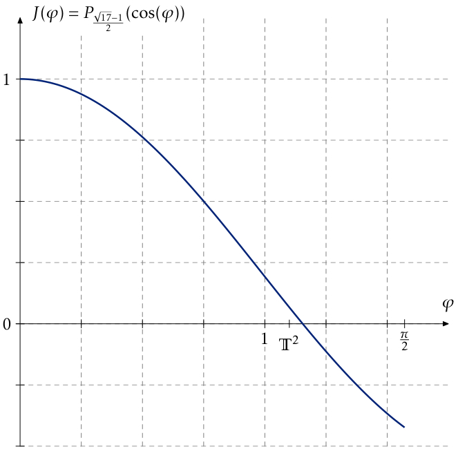
Figure 3. Jacobi field J𝐽J on S3𝕊2subscript𝑆3superscript𝕊2S_{3}\subseteq\mathbb{S}^{2}, with Neumann condition on {x=0}𝑥0\{x=0\}. Drawn w.r.t. polar coordinates around (0,1)01(0,1), where φ𝜑\varphi is the angle out from the x2subscript𝑥2x_{2}-axis in Figure 2. Point of intersection with 𝕋2superscript𝕋2\mathbb{T}^{2} indicated.
Refer to caption
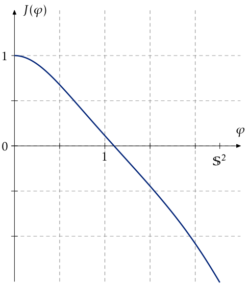
Figure 4. Jacobi field J𝐽J on S5𝕋2subscript𝑆5superscript𝕋2S_{5}\subseteq\mathbb{T}^{2}, with Neumann condition on {x=0}𝑥0\{x=0\}. Drawn w.r.t. polar coordinates around (0,1)01(0,1), where φ𝜑\varphi is the angle out from the x2subscript𝑥2x_{2}-axis in Figure 2. Point of intersection with 𝕊2superscript𝕊2\mathbb{S}^{2} indicated.
Refer to caption
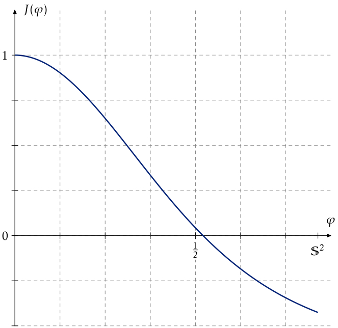
Figure 5. Jacobi field J𝐽J on S6𝕋2subscript𝑆6superscript𝕋2S_{6}\subseteq\mathbb{T}^{2}, with Neumann condition on {x=0}𝑥0\{x=0\}. Drawn w.r.t. polar coordinates around (0,1)01(0,1), where φ𝜑\varphi is the angle out from the x2subscript𝑥2x_{2}-axis in Figure 2. Point of intersection with 𝕊2superscript𝕊2\mathbb{S}^{2} indicated.
Lemma 2.10.

For graphs of the form (x1,u(x1))subscript𝑥1𝑢subscript𝑥1(x_{1},u(x_{1})) the operator 0subscript0\mathcal{L}_{0} specializes to ω=1+(u)2𝜔1superscriptsuperscript𝑢2\omega=1+(u^{\prime})^{2}, and

ω0v𝜔subscript0𝑣\displaystyle\omega\mathcal{L}_{0}v =v′′x12(1+(u)2)v+[(ux1u21u)2+1u2+1+(u)22]v,absentsuperscript𝑣′′subscript𝑥121superscriptsuperscript𝑢2superscript𝑣delimited-[]superscript𝑢subscript𝑥1superscript𝑢21𝑢21superscript𝑢21superscriptsuperscript𝑢22𝑣\displaystyle=v^{\prime\prime}-\frac{x_{1}}{2}\left(1+(u^{\prime})^{2}\right)v^{\prime}+\left[\left(\frac{u-x_{1}u^{\prime}}{2}-\frac{1}{u}\right)^{2}+\frac{1}{u^{2}}+\frac{1+(u^{\prime})^{2}}{2}\right]v,
=:v′′+P(x1,u,u)v+Q(x1,u,u)v,\displaystyle=:v^{\prime\prime}+P(x_{1},u,u^{\prime})v^{\prime}+Q(x_{1},u,u^{\prime})v,

when u𝑢u is a solution to the shrinker equation.

For solution graphs of the form (f(x2),x2)𝑓subscript𝑥2subscript𝑥2(f(x_{2}),x_{2}) we have ω=1+(f)2𝜔1superscriptsuperscript𝑓2\omega=1+(f^{\prime})^{2} and the formula is:

ω0g𝜔subscript0𝑔\displaystyle\omega\mathcal{L}_{0}g =g′′+[1x2x22](1+(f)2)g+[(x2ff2fx2)2+(f)2x22+1+(f)22]gabsentsuperscript𝑔′′delimited-[]1subscript𝑥2subscript𝑥221superscriptsuperscript𝑓2superscript𝑔delimited-[]superscriptsubscript𝑥2superscript𝑓𝑓2superscript𝑓subscript𝑥22superscriptsuperscript𝑓2superscriptsubscript𝑥221superscriptsuperscript𝑓22𝑔\displaystyle=g^{\prime\prime}+\left[\frac{1}{x_{2}}-\frac{x_{2}}{2}\right]\left(1+(f^{\prime})^{2}\right)g^{\prime}+\left[\left(\frac{x_{2}f^{\prime}-f}{2}-\frac{f^{\prime}}{x_{2}}\right)^{2}+\frac{(f^{\prime})^{2}}{x_{2}^{2}}+\frac{1+(f^{\prime})^{2}}{2}\right]g
=:g′′+R(x2,f,f)g+S(x2,f,f)g.\displaystyle=:g^{\prime\prime}+R(x_{2},f,f^{\prime})g^{\prime}+S(x_{2},f,f^{\prime})g.

Let us as a preliminary consideration note that the mean curvature H𝐻H has rotational symmetry, and is an eigenfunction with eigenvalue 111 (see [CM2]):

(2.51) H=H,𝐻𝐻\mathcal{L}H=H,

and Neumann conditions on {x1=0}subscript𝑥10\{x_{1}=0\}. The profile of 𝕋2superscript𝕋2\mathbb{T}^{2} is convex as shown in [KMø], and thus since the sign of the mean curvature changes only at points of tangential contact with a straight line from the origin, we see that on 𝕋2superscript𝕋2\mathbb{T}^{2} the function Hγ𝐻𝛾H\circ\gamma has exactly one zero.

By Sturm-Liouville theory, we now conclude from (2.51) that a solution to the Neumann problem for 0subscript0\mathcal{L}_{0}, if it exists, needs to have at least two zeros in the interval. However, it of course turns out there are no such non-trivial fields with Neumann conditions, which is what we now will apply more detailed analysis to show.

2.2.1. Surfaces contained in 𝕊2superscript𝕊2\mathbb{S}^{2}

For surfaces contained in 𝕊2superscript𝕊2\mathbb{S}^{2} it is of natural convenience to use polar coordinates. Recall that a curve (ρ,φ),φ=arctan(x/z)𝜌𝜑𝜑𝑥𝑧(\rho,\varphi),\varphi=\arctan(x/z) in the xz𝑥𝑧xz-plane generated by a function ρ(φ)𝜌𝜑\rho(\varphi) that generates a smooth solution to the self-shrinker equation (2.32) satisfies:

(2.52) ρ′′(φ)=1ρ{ρ2+2(ρ)2+[1ρ22ρρtanφ](ρ2+(ρ)2)}.superscript𝜌′′𝜑1𝜌superscript𝜌22superscriptsuperscript𝜌2delimited-[]1superscript𝜌22superscript𝜌𝜌𝜑superscript𝜌2superscriptsuperscript𝜌2\rho^{\prime\prime}(\varphi)=\frac{1}{\rho}\left\{\rho^{2}+2(\rho^{\prime})^{2}+\Big{[}1-\frac{\rho^{2}}{2}-\frac{\rho^{\prime}}{\rho\tan\varphi}\Big{]}\big{(}\rho^{2}+(\rho^{\prime})^{2}\big{)}\right\}.

A function w𝑤w giving a (via a unit normal w.r.t. Euclidean length) variation field, must thus on 𝕊2superscript𝕊2\mathbb{S}^{2} satisfy the equation (see Appendix A in [KKMø])

(2.53) w′′+1tanφw+4w=0,superscript𝑤′′1𝜑superscript𝑤4𝑤0w^{\prime\prime}+\frac{1}{\tan\varphi}w^{\prime}+4w=0,

with appropriate boundary conditions. The substitution x=cos(φ)𝑥𝜑x=\cos(\varphi) in (2.53) gives Legendre’s differential equation, and the solution is:

w(φ)=C1Pl0(cosφ)+C2Ql0(cosφ),𝑤𝜑subscript𝐶1subscript𝑃subscript𝑙0𝜑subscript𝐶2subscript𝑄subscript𝑙0𝜑w(\varphi)=C_{1}P_{l_{0}}(\cos\varphi)+C_{2}Q_{l_{0}}(\cos\varphi),

where Plsubscript𝑃𝑙P_{l} and Qlsubscript𝑄𝑙Q_{l} are respectively the Legendre functions of the first and second kind, and l0=(171)/2subscript𝑙01712l_{0}=(\sqrt{17}-1)/2 is the positive root of l(l+1)=4𝑙𝑙14l(l+1)=4.

For the surface S1𝕊2subscript𝑆1superscript𝕊2S_{1}\subseteq\mathbb{S}^{2}, which is generated by rotation of the radius 2 quarter-circle, the boundary conditions in the theorem are w(0)=0superscript𝑤00w^{\prime}(0)=0 and w(π2)=0superscript𝑤matrix𝜋20w^{\prime}(\begin{matrix}\frac{\pi}{2}\end{matrix})=0. But since Ql0(cosφ)subscript𝑄subscript𝑙0𝜑Q_{l_{0}}(\cos\varphi) has a pole at φ=0𝜑0\varphi=0, we see that C2=0subscript𝐶20C_{2}=0. Thus, if we normalize w𝑤w so that C1=1subscript𝐶11C_{1}=1, we have by the first condition that w=Pl0(cosφ)𝑤subscript𝑃subscript𝑙0𝜑w=P_{l_{0}}(\cos\varphi). However,

(2.54) dPl0(cosφ)dφφ=π2=π217+1Γ(1174)Γ(5+174)0,\frac{dP_{l_{0}}(\cos\varphi)}{d\varphi}_{\mid\varphi=\begin{matrix}\frac{\pi}{2}\end{matrix}}=\frac{\sqrt{\pi}}{2}\frac{\sqrt{17}+1}{\Gamma\left(\frac{1-\sqrt{17}}{4}\right)\Gamma\left(\frac{5+\sqrt{17}}{4}\right)}\neq 0,

and hence there is no such Neumann mode. By the preceding, we therefore conclude that under N𝑁N-fold symmetry, for a large enough N>0𝑁0N>0,

(2.55) kerS1={0},onS1=𝕊2{x10}[Neumann conditions].formulae-sequencekernelsubscriptsubscript𝑆10onsubscript𝑆1superscript𝕊2subscript𝑥10[Neumann conditions]\ker\mathcal{L}_{S_{1}}=\{0\},\quad\textrm{on}\quad S_{1}=\mathbb{S}^{2}\cap\{x_{1}\geq 0\}\quad\textrm{[Neumann conditions]}.

As for the surface S3𝕊2subscript𝑆3superscript𝕊2S_{3}\subseteq\mathbb{S}^{2}, which we let for definiteness be the component such that (2,0)S320subscript𝑆3(2,0)\in S_{3}, again C1=1subscript𝐶11C_{1}=1 and C2=0subscript𝐶20C_{2}=0. Now, since by (2.4),

(2.56) Pl0(cos((e1,p+)))Pl0(cos(1110+120))1200>0,subscript𝑃subscript𝑙0subscript𝑒1superscript𝑝subscript𝑃subscript𝑙0matrix1110matrix120matrix12000P_{l_{0}}(\cos(\angle(\vec{e_{1}},p^{+})))\geq P_{l_{0}}(\cos(\begin{matrix}\frac{11}{10}\end{matrix}+\begin{matrix}\frac{1}{20}\end{matrix}))\geq\begin{matrix}\frac{1}{200}\end{matrix}>0,

we conclude again

(2.57) kerS3={0}[Dirichlet conditions].kernelsubscriptsubscript𝑆30[Dirichlet conditions]\ker\mathcal{L}_{S_{3}}=\{0\}\quad\textrm{[Dirichlet conditions]}.

For S4𝕊2subscript𝑆4superscript𝕊2S_{4}\subseteq\mathbb{S}^{2}, the component with (0,2)S402subscript𝑆4(0,2)\in S_{4}, we see that with w(π2)=0superscript𝑤matrix𝜋20w^{\prime}(\begin{matrix}\frac{\pi}{2}\end{matrix})=0 and fixing w(π2)=1𝑤matrix𝜋21w(\begin{matrix}\frac{\pi}{2}\end{matrix})=1,

(C1C2)=(Pl0(cos(π2))Ql0(cos(π2))ddφPl0(cos(π2))ddφPl0(cos(π2)))1(10)matrixsubscript𝐶1subscript𝐶2superscriptmatrixsubscript𝑃subscript𝑙0matrix𝜋2subscript𝑄subscript𝑙0matrix𝜋2matrix𝑑𝑑𝜑subscript𝑃subscript𝑙0matrix𝜋2matrix𝑑𝑑𝜑subscript𝑃subscript𝑙0matrix𝜋21matrix10\begin{pmatrix}C_{1}\\ C_{2}\end{pmatrix}=\begin{pmatrix}P_{l_{0}}(\cos(\begin{matrix}\frac{\pi}{2}\end{matrix}))&Q_{l_{0}}(\cos(\begin{matrix}\frac{\pi}{2}\end{matrix}))\\ \begin{matrix}\frac{d}{d\varphi}\end{matrix}P_{l_{0}}(\cos(\begin{matrix}\frac{\pi}{2}\end{matrix}))&\begin{matrix}\frac{d}{d\varphi}\end{matrix}P_{l_{0}}(\cos(\begin{matrix}\frac{\pi}{2}\end{matrix}))\end{pmatrix}^{-1}\begin{pmatrix}1\\ 0\end{pmatrix}

such that with these constants

w((e1,p+))w(1110)100εgap>12>0.𝑤subscript𝑒1superscript𝑝𝑤matrix1110100subscript𝜀gapmatrix120w(\angle(\vec{e_{1}},p^{+}))\geq w(\begin{matrix}\frac{11}{10}\end{matrix})-100\varepsilon_{\textrm{gap}}>\begin{matrix}\frac{1}{2}\end{matrix}>0.

Thus on the surface S4subscript𝑆4S_{4} with Neumann and Dirichlet conditions as in the statement of the theorem, we also conclude

(2.58) kerS4={0}[Neumann on {x1=0}, Dirichlet on S4𝕋2].kernelsubscriptsubscript𝑆40[Neumann on {x1=0}, Dirichlet on S4𝕋2]\ker\mathcal{L}_{S_{4}}=\{0\}\quad\textrm{[Neumann on $\{x_{1}=0\}$, Dirichlet on $S_{4}\cap\mathbb{T}^{2}$]}.

2.2.2. Surfaces Contained in 𝕋2superscript𝕋2\mathbb{T}^{2}

In this section we will show that the Jacobi fields with Neumann conditions u0(0)=0superscriptsubscript𝑢000u_{0}^{\prime}(0)=0 (and normalized to u0(0)=1subscript𝑢001u_{0}(0)=1), propagated from respectively the top and the bottom of the torus 𝕋2superscript𝕋2\mathbb{T}^{2} from Section 2 have the following end-point values at the point where 𝕋2superscript𝕋2\mathbb{T}^{2} intersects the round 2-sphere of radius 222:

(2.59) (u0(ttop)u0(ttop))=(2250±10εgap3750±10εgap)matrixsubscript𝑢0subscript𝑡topsuperscriptsubscript𝑢0subscript𝑡topmatrixplus-or-minusmatrix225010subscript𝜀gapmissing-subexpressionplus-or-minusmatrix375010subscript𝜀gap\begin{pmatrix}u_{0}(t_{\textrm{top}})\\ u_{0}^{\prime}(t_{\textrm{top}})\end{pmatrix}=\begin{pmatrix}-\begin{matrix}\frac{22}{50}\end{matrix}\pm 10\varepsilon_{\mathrm{gap}}\\ \hbox{}\\ -\begin{matrix}\frac{37}{50}\end{matrix}\pm 10\varepsilon_{\mathrm{gap}}\end{pmatrix}

and

(2.60) (u0(tbot)u0(tbot))=(7750±10εgap8450±10εgap,)matrixsubscript𝑢0subscript𝑡botsuperscriptsubscript𝑢0subscript𝑡botmatrixplus-or-minusmatrix775010subscript𝜀gapmissing-subexpressionplus-or-minusmatrix845010subscript𝜀gap\begin{pmatrix}u_{0}(t_{\textrm{bot}})\\ u_{0}^{\prime}(t_{\textrm{bot}})\end{pmatrix}=\begin{pmatrix}-\begin{matrix}\frac{77}{50}\end{matrix}\pm 10\varepsilon_{\mathrm{gap}}\\ \hbox{}\\ -\begin{matrix}\frac{84}{50}\end{matrix}\pm 10\varepsilon_{\mathrm{gap}},\end{pmatrix}

where the notation is meant to imply that each component is contained in the corresponding intervals arising from both choices of sign.

This means firstly that the Dirichlet problems on each part (w/ Neumann conditions on 𝒫𝒫\mathcal{P}) have trivial kernel, that is:

(2.61) kerS5={0}[Neumann on {x1=0}, Dirichlet on S5𝕊2],kernelsubscriptsubscript𝑆50[Neumann on {x1=0}, Dirichlet on S5𝕊2]\displaystyle\ker\mathcal{L}_{S_{5}}=\{0\}\quad\textrm{[Neumann on $\{x_{1}=0\}$, Dirichlet on $S_{5}\cap\mathbb{S}^{2}$]},
(2.62) kerS6={0}[Neumann on {x1=0}, Dirichlet on S6𝕊2].kernelsubscriptsubscript𝑆60[Neumann on {x1=0}, Dirichlet on S6𝕊2]\displaystyle\ker\mathcal{L}_{S_{6}}=\{0\}\quad\textrm{[Neumann on $\{x_{1}=0\}$, Dirichlet on $S_{6}\cap\mathbb{S}^{2}$]}.

Secondly, note that non-triviality of the kernel of \mathcal{L} on 𝕋2{x10}superscript𝕋2subscript𝑥10\mathbb{T}^{2}\cap\{x_{1}\geq 0\} with Neumann conditions has now been reduced to the conditions

αu0(ttop)=βu0(ttop),𝛼subscript𝑢0subscript𝑡top𝛽subscript𝑢0subscript𝑡top\displaystyle\alpha u_{0}(t_{\textrm{top}})=\beta u_{0}(t_{\textrm{top}}),
αu0(ttop)=βu0(tbot),𝛼superscriptsubscript𝑢0subscript𝑡top𝛽superscriptsubscript𝑢0subscript𝑡bot\displaystyle\alpha u_{0}^{\prime}(t_{\textrm{top}})=-\beta u_{0}^{\prime}(t_{\textrm{bot}}),

for a non-zero pair (α,β)𝛼𝛽(\alpha,\beta) or in other words, singularity of the matrix 𝒩𝒩\mathcal{N}:

(2.63) 𝒩:=(u0(ttop)u0(tbot)u0(ttop)u0(tbot)).assign𝒩matrixsubscript𝑢0subscript𝑡topsubscript𝑢0subscript𝑡botsuperscriptsubscript𝑢0subscript𝑡topsuperscriptsubscript𝑢0subscript𝑡bot\mathcal{N}:=\begin{pmatrix}u_{0}(t_{\textrm{top}})&-u_{0}(t_{\textrm{bot}})\\ u_{0}^{\prime}(t_{\textrm{top}})&u_{0}^{\prime}(t_{\textrm{bot}})\end{pmatrix}.

But in fact from (2.59)–(2.60) we see

(2.64) det𝒩95>0,𝒩matrix950\det\mathcal{N}\geq\begin{matrix}\frac{9}{5}\end{matrix}>0,

so we finally conclude that also

kerS2={0}[Neumann on {x1=0}.kernelsubscriptsubscript𝑆20[Neumann on {x1=0}\ker\mathcal{L}_{S_{2}}=\{0\}\quad\textrm{[Neumann on $\{x_{1}=0\}$}.

To show the required estimates of the Jacobi fields, we consider first an approximate solution V𝑉V to the linearized equation on the approximate curve ΓΓ\Gamma from the previous section.

Top: x1subscript𝑥1x_{1}-graph (Jacobi Equation)

Let us consider the first part of ΓΓ\Gamma, graphical over the x1subscript𝑥1x_{1}-axis, on x1[0,35]subscript𝑥10matrix35x_{1}\in[0,\begin{matrix}\frac{3}{5}\end{matrix}]. Here, we have the expressions (recall Lemma 2.10 for the definition of P𝑃P an Q𝑄Q).

|2P(x1,ξ,U)|=0,subscript2𝑃subscript𝑥1𝜉superscript𝑈0\displaystyle\left|\partial_{2}P(x_{1},\xi,U^{\prime})\right|=0,
|3P(x1,u,ξ)|=|x1ξ|,subscript3𝑃subscript𝑥1𝑢superscript𝜉subscript𝑥1superscript𝜉\displaystyle\left|\partial_{3}P(x_{1},u,\xi^{\prime})\right|=|x_{1}\xi^{\prime}|,
|2Q(x1,ξ,U)|=2|(ξx1U21ξ)(12+1ξ2)1ξ3|,subscript2𝑄subscript𝑥1𝜉superscript𝑈2𝜉subscript𝑥1superscript𝑈21𝜉121superscript𝜉21superscript𝜉3\displaystyle\left|\partial_{2}Q(x_{1},\xi,U^{\prime})\right|=2\left|\left(\frac{\xi-x_{1}U^{\prime}}{2}-\frac{1}{\xi}\right)\left(\frac{1}{2}+\frac{1}{\xi^{2}}\right)-\frac{1}{\xi^{3}}\right|,
|3Q(x1,u,ξ)|=|x1(ux1ξ21u)ξ|.subscript3𝑄subscript𝑥1𝑢superscript𝜉subscript𝑥1𝑢subscript𝑥1superscript𝜉21𝑢superscript𝜉\displaystyle\left|\partial_{3}Q(x_{1},u,\xi^{\prime})\right|=\left|x_{1}\left(\frac{u-x_{1}\xi^{\prime}}{2}-\frac{1}{u}\right)-\xi^{\prime}\right|.

Assume for a small δ1T>0superscriptsubscript𝛿1𝑇0\delta_{1}^{T}>0 the uniform bounds:

(2.65) |V′′+P(x1,U,U)V+Q(x1,U,U)V|δ1T,superscript𝑉′′𝑃subscript𝑥1𝑈superscript𝑈superscript𝑉𝑄subscript𝑥1𝑈superscript𝑈𝑉superscriptsubscript𝛿1𝑇\displaystyle\left|V^{\prime\prime}+P(x_{1},U,U^{\prime})V^{\prime}+Q(x_{1},U,U^{\prime})V\right|\leq\delta_{1}^{T},
(2.66) |3P(x1,u,ξ)||v|+|3Q(x1,u,ξ)||v|x1(2x12+3),subscript3𝑃subscript𝑥1𝑢superscript𝜉superscript𝑣subscript3𝑄subscript𝑥1𝑢superscript𝜉𝑣subscript𝑥12superscriptsubscript𝑥123\displaystyle\left|\partial_{3}P(x_{1},u,\xi^{\prime})\right||v^{\prime}|+\left|\partial_{3}Q(x_{1},u,\xi^{\prime})\right||v|\leq x_{1}(2x_{1}^{2}+3),
(2.67) |2Q(x1,ξ,U)||v|8532x12.subscript2𝑄subscript𝑥1𝜉superscript𝑈𝑣matrix85matrix32superscriptsubscript𝑥12\displaystyle\left|\partial_{2}Q(x_{1},\xi,U^{\prime})\right||v|\leq\begin{matrix}\frac{8}{5}\end{matrix}-\begin{matrix}\frac{3}{2}\end{matrix}x_{1}^{2}.

We let Φ(x1):=|V(x1)v(x1)|assignΦsubscript𝑥1superscript𝑉subscript𝑥1superscript𝑣subscript𝑥1\Phi(x_{1}):=|V^{\prime}(x_{1})-v^{\prime}(x_{1})| and estimate:

Φ(x1)superscriptΦsubscript𝑥1\displaystyle\Phi^{\prime}(x_{1}) ||Vv||=a.e|V′′v′′|absentsuperscriptsuperscript𝑉superscript𝑣a.esuperscript𝑉′′superscript𝑣′′\displaystyle\leq\left||V^{\prime}-v^{\prime}|^{\prime}\right|\overset{\textrm{a.e}}{=}|V^{\prime\prime}-v^{\prime\prime}|
|P(x1,U,U)VP(x1,u,u)v|+|Q(x1,U,U)VQ(x1,u,u)v|+δ1Tabsent𝑃subscript𝑥1𝑈superscript𝑈superscript𝑉𝑃subscript𝑥1𝑢superscript𝑢superscript𝑣𝑄subscript𝑥1𝑈superscript𝑈𝑉𝑄subscript𝑥1𝑢superscript𝑢𝑣superscriptsubscript𝛿1𝑇\displaystyle\leq\left|P(x_{1},U,U^{\prime})V^{\prime}-P(x_{1},u,u^{\prime})v^{\prime}\right|+\left|Q(x_{1},U,U^{\prime})V-Q(x_{1},u,u^{\prime})v\right|+\delta_{1}^{T}
|P(x1,U,U)||Vv|+|P(x1,U,U)P(x1,u,u)||v|absent𝑃subscript𝑥1𝑈superscript𝑈superscript𝑉superscript𝑣𝑃subscript𝑥1𝑈superscript𝑈𝑃subscript𝑥1𝑢superscript𝑢superscript𝑣\displaystyle\leq\left|P(x_{1},U,U^{\prime})\right||V^{\prime}-v^{\prime}|+\left|P(x_{1},U,U^{\prime})-P(x_{1},u,u^{\prime})\right||v^{\prime}|
+|Q(x1,U,U)||Vv|+|Q(x1,U,U)Q(x1,u,u)||v|+δ1T𝑄subscript𝑥1𝑈superscript𝑈𝑉𝑣𝑄subscript𝑥1𝑈superscript𝑈𝑄subscript𝑥1𝑢superscript𝑢𝑣superscriptsubscript𝛿1𝑇\displaystyle\qquad+\left|Q(x_{1},U,U^{\prime})\right||V-v|+\left|Q(x_{1},U,U^{\prime})-Q(x_{1},u,u^{\prime})\right||v|+\delta_{1}^{T}
|P(x1,U,U)||Vv|+|Q(x1,U,U)||Vv|absent𝑃subscript𝑥1𝑈superscript𝑈superscript𝑉superscript𝑣𝑄subscript𝑥1𝑈superscript𝑈𝑉𝑣\displaystyle\leq\left|P(x_{1},U,U^{\prime})\right||V^{\prime}-v^{\prime}|+\left|Q(x_{1},U,U^{\prime})\right||V-v|
+(|3P(x1,u,ξ)||v|+|3Q(x1,u,ξ)||v|)|Uu|subscript3𝑃subscript𝑥1𝑢superscript𝜉superscript𝑣subscript3𝑄subscript𝑥1𝑢superscript𝜉𝑣superscript𝑈superscript𝑢\displaystyle\qquad+\left(\left|\partial_{3}P(x_{1},u,\xi^{\prime})\right||v^{\prime}|+\left|\partial_{3}Q(x_{1},u,\xi^{\prime})\right||v|\right)|U^{\prime}-u^{\prime}|
+(|2P(x1,ξ,U)||v|+|2Q(x1,ξ,U)||v|)|Uu|+δ1Tcancelsubscript2𝑃subscript𝑥1𝜉superscript𝑈superscript𝑣subscript2𝑄subscript𝑥1𝜉superscript𝑈𝑣𝑈𝑢superscriptsubscript𝛿1𝑇\displaystyle\qquad+\left(\cancel{\left|\partial_{2}P(x_{1},\xi,U^{\prime})\right|}|v^{\prime}|+\left|\partial_{2}Q(x_{1},\xi,U^{\prime})\right||v|\right)|U-u|+\delta_{1}^{T}
|P(x1,U,U)|Φ(x1)+|Q(x1,U,U)|0x1Φ(s)𝑑s+|Q(x1,U,U)||V(0)v(0)|absent𝑃subscript𝑥1𝑈superscript𝑈Φsubscript𝑥1𝑄subscript𝑥1𝑈superscript𝑈superscriptsubscript0subscript𝑥1Φ𝑠differential-d𝑠𝑄subscript𝑥1𝑈superscript𝑈𝑉0𝑣0\displaystyle\leq\left|P(x_{1},U,U^{\prime})\right|\Phi(x_{1})+\left|Q(x_{1},U,U^{\prime})\right|\int_{0}^{x_{1}}\Phi(s)ds+\left|Q(x_{1},U,U^{\prime})\right||V(0)-v(0)|
+x1(2x12+3)|U(x1)u(x1)|+(8532x12)|U(x1)u(x1)|+δ1T.subscript𝑥12superscriptsubscript𝑥123superscript𝑈subscript𝑥1superscript𝑢subscript𝑥1matrix85matrix32superscriptsubscript𝑥12𝑈subscript𝑥1𝑢subscript𝑥1superscriptsubscript𝛿1𝑇\displaystyle\qquad+x_{1}(2x_{1}^{2}+3)|U^{\prime}(x_{1})-u^{\prime}(x_{1})|+(\begin{matrix}\frac{8}{5}\end{matrix}-\begin{matrix}\frac{3}{2}\end{matrix}x_{1}^{2})|U(x_{1})-u(x_{1})|+\delta_{1}^{T}.

We integrate on [0,x1]0subscript𝑥1[0,x_{1}] to get:

Φ(x1)Φsubscript𝑥1absent\displaystyle\Phi(x_{1})\leq 0x1[|P(s,U,U)|+0x1|Q(t,U,U)|𝑑t]Φ(s)𝑑s+(0x1|Q(s,U,U)|𝑑s)|V(0)v(0)|superscriptsubscript0subscript𝑥1delimited-[]𝑃𝑠𝑈superscript𝑈superscriptsubscript0subscript𝑥1𝑄𝑡𝑈superscript𝑈differential-d𝑡Φ𝑠differential-d𝑠superscriptsubscript0subscript𝑥1𝑄𝑠𝑈superscript𝑈differential-d𝑠𝑉0𝑣0\displaystyle\int_{0}^{x_{1}}\left[\left|P(s,U,U^{\prime})\right|+\int_{0}^{x_{1}}\left|Q(t,U,U^{\prime})\right|dt\right]\Phi(s)ds+\left(\int_{0}^{x_{1}}\left|Q(s,U,U^{\prime})\right|ds\right)|V(0)-v(0)|
+0x1s(2s2+3)|U(s)u(s)|𝑑s+0x1(8532s2)|U(s)u(s)|𝑑s+δ1Tx1.superscriptsubscript0subscript𝑥1𝑠2superscript𝑠23superscript𝑈𝑠superscript𝑢𝑠differential-d𝑠superscriptsubscript0subscript𝑥1matrix85matrix32superscript𝑠2𝑈𝑠𝑢𝑠differential-d𝑠subscriptsuperscript𝛿𝑇1subscript𝑥1\displaystyle\quad+\int_{0}^{x_{1}}s(2s^{2}+3)|U^{\prime}(s)-u^{\prime}(s)|ds+\int_{0}^{x_{1}}(\begin{matrix}\frac{8}{5}\end{matrix}-\begin{matrix}\frac{3}{2}\end{matrix}s^{2})|U(s)-u(s)|ds+\delta^{T}_{1}x_{1}.

Recall the estimates for |U(s)u(s)|superscript𝑈𝑠superscript𝑢𝑠|U^{\prime}(s)-u^{\prime}(s)|, which lead to:

0x1s(2s2+3)|U(s)u(s)|𝑑ssuperscriptsubscript0subscript𝑥1𝑠2superscript𝑠23superscript𝑈𝑠superscript𝑢𝑠differential-d𝑠\displaystyle\int_{0}^{x_{1}}s(2s^{2}+3)|U^{\prime}(s)-u^{\prime}(s)|ds [45|U(0)u(0)|+ε1T]0x1s2(2s2+3)exp{5215s2}𝑑sabsentdelimited-[]matrix45𝑈0𝑢0superscriptsubscript𝜀1𝑇superscriptsubscript0subscript𝑥1superscript𝑠22superscript𝑠23matrix5215superscript𝑠2differential-d𝑠\displaystyle\leq\left[\begin{matrix}\frac{4}{5}\end{matrix}|U(0)-u(0)|+\varepsilon_{1}^{T}\right]\int_{0}^{x_{1}}s^{2}(2s^{2}+3)\exp\Big{\{}\begin{matrix}\frac{52}{15}\end{matrix}s^{2}\Big{\}}ds
920|U(0)u(0)|+1425ε1T.absentmatrix920𝑈0𝑢0matrix1425subscriptsuperscript𝜀𝑇1\displaystyle\leq\begin{matrix}\frac{9}{20}\end{matrix}|U(0)-u(0)|+\begin{matrix}\frac{14}{25}\end{matrix}\varepsilon^{T}_{1}.

Note also that from the estimates for |Uu|𝑈𝑢|U-u| from |Uu|superscript𝑈superscript𝑢|U^{\prime}-u^{\prime}|, we have already once estimated the integral of the latter. We now need the sizes of these elementary Gaussian double integrals:

035(8532x12)(1+0x14s5exp{5215s2}𝑑s)𝑑x12325,superscriptsubscript0matrix35matrix85matrix32superscriptsubscript𝑥121superscriptsubscript0subscript𝑥1matrix4𝑠5matrix5215superscript𝑠2differential-d𝑠differential-dsubscript𝑥12325\displaystyle\int_{0}^{\begin{matrix}\frac{3}{5}\end{matrix}}(\begin{matrix}\frac{8}{5}\end{matrix}-\begin{matrix}\frac{3}{2}\end{matrix}x_{1}^{2})\left(1+\int_{0}^{x_{1}}\begin{matrix}\frac{4s}{5}\end{matrix}\exp\Big{\{}\begin{matrix}\frac{52}{15}\end{matrix}s^{2}\Big{\}}ds\right)dx_{1}\leq\frac{23}{25},
035(8532x12)0x1sexp{5215s2}𝑑s𝑑x17100.superscriptsubscript0matrix35matrix85matrix32superscriptsubscript𝑥12superscriptsubscript0subscript𝑥1𝑠matrix5215superscript𝑠2differential-d𝑠differential-dsubscript𝑥17100\displaystyle\int_{0}^{\begin{matrix}\frac{3}{5}\end{matrix}}(\begin{matrix}\frac{8}{5}\end{matrix}-\begin{matrix}\frac{3}{2}\end{matrix}x_{1}^{2})\int_{0}^{x_{1}}s\exp\Big{\{}\begin{matrix}\frac{52}{15}\end{matrix}s^{2}\Big{\}}dsdx_{1}\leq\frac{7}{100}.

Thus

035(8532s2)|U(s)u(s)|𝑑s2325|U(0)u(0)|+7100ε1T.superscriptsubscript0matrix35matrix85matrix32superscript𝑠2𝑈𝑠𝑢𝑠differential-d𝑠matrix2325𝑈0𝑢0matrix7100subscriptsuperscript𝜀𝑇1\int_{0}^{\begin{matrix}\frac{3}{5}\end{matrix}}(\begin{matrix}\frac{8}{5}\end{matrix}-\begin{matrix}\frac{3}{2}\end{matrix}s^{2})|U(s)-u(s)|ds\leq\begin{matrix}\frac{23}{25}\end{matrix}|U(0)-u(0)|+\begin{matrix}\frac{7}{100}\end{matrix}\varepsilon^{T}_{1}.

Now, we will furthermore assume the following bounds on the test functions, pertaining to the approximation by ε𝜀\varepsilon-geodesics:

(2.68) 0x1|P(s,U,U)|𝑑s0x1s(75s2+710)𝑑s720x12(x12+1),superscriptsubscript0subscript𝑥1𝑃𝑠𝑈superscript𝑈differential-d𝑠superscriptsubscript0subscript𝑥1𝑠matrix75superscript𝑠2matrix710differential-d𝑠matrix720superscriptsubscript𝑥12superscriptsubscript𝑥121\displaystyle\int_{0}^{x_{1}}|P(s,U,U^{\prime})|ds\leq\int_{0}^{x_{1}}s(\begin{matrix}\frac{7}{5}\end{matrix}s^{2}+\begin{matrix}\frac{7}{10}\end{matrix})ds\leq\begin{matrix}\frac{7}{20}\end{matrix}x_{1}^{2}(x_{1}^{2}+1),
(2.69) 0x1|Q(s,U,U)|𝑑s0x1(165s2+52)𝑑s1615x13+52x1.superscriptsubscript0subscript𝑥1𝑄𝑠𝑈superscript𝑈differential-d𝑠superscriptsubscript0subscript𝑥1matrix165superscript𝑠2matrix52differential-d𝑠matrix1615superscriptsubscript𝑥13matrix52subscript𝑥1\displaystyle\int_{0}^{x_{1}}\left|Q(s,U,U^{\prime})\right|ds\leq\int_{0}^{x_{1}}(\begin{matrix}\frac{16}{5}\end{matrix}s^{2}+\begin{matrix}\frac{5}{2}\end{matrix})ds\leq\begin{matrix}\frac{16}{15}\end{matrix}x_{1}^{3}+\begin{matrix}\frac{5}{2}\end{matrix}x_{1}.

Applying Grönwall-Bellman again, to these new estimates, we see, using also that V(0)=v(0)=1𝑉0𝑣01V(0)=v(0)=1 by assumption:

Φ(x1)Φsubscript𝑥1absent\displaystyle\Phi(x_{1})\leq [0x1s(2s2+3)|U(s)u(s)|ds+0x1(8532s2)|U(s)u(s)|ds+δ1Tx1]×\displaystyle\left[\int_{0}^{x_{1}}s(2s^{2}+3)|U^{\prime}(s)-u^{\prime}(s)|ds+\int_{0}^{x_{1}}(\begin{matrix}\frac{8}{5}\end{matrix}-\begin{matrix}\frac{3}{2}\end{matrix}s^{2})|U(s)-u(s)|ds+\delta^{T}_{1}x_{1}\right]\times
exp{0x1|P(s,U,U)|𝑑s+x10x1|Q(s,U,U)|𝑑s}superscriptsubscript0subscript𝑥1𝑃𝑠𝑈superscript𝑈differential-d𝑠subscript𝑥1superscriptsubscript0subscript𝑥1𝑄𝑠𝑈superscript𝑈differential-d𝑠\displaystyle\qquad\exp\left\{\int_{0}^{x_{1}}\left|P(s,U,U^{\prime})\right|ds+x_{1}\int_{0}^{x_{1}}\left|Q(s,U,U^{\prime})\right|ds\right\}
\displaystyle\leq [137100|U(0)u(0)|+63100ε1T+35δ1T]×\displaystyle\left[\begin{matrix}\frac{137}{100}\end{matrix}|U(0)-u(0)|+\begin{matrix}\frac{63}{100}\end{matrix}\varepsilon^{T}_{1}+\begin{matrix}\frac{3}{5}\end{matrix}\delta^{T}_{1}\right]\times
exp{720x12(x12+1)+1615x14+52x12}.matrix720superscriptsubscript𝑥12superscriptsubscript𝑥121matrix1615superscriptsubscript𝑥14matrix52superscriptsubscript𝑥12\displaystyle\qquad\exp\left\{\begin{matrix}\frac{7}{20}\end{matrix}x_{1}^{2}(x_{1}^{2}+1)+\begin{matrix}\frac{16}{15}\end{matrix}x_{1}^{4}+\begin{matrix}\frac{5}{2}\end{matrix}x_{1}^{2}\right\}.

Thus

|V(35)v(35)|235|U(0)u(0)|+115ε1T+5125δ1T,superscript𝑉matrix35superscript𝑣matrix35matrix235𝑈0𝑢0matrix115superscriptsubscript𝜀1𝑇matrix5125superscriptsubscript𝛿1𝑇\displaystyle|V^{\prime}(\begin{matrix}\frac{3}{5}\end{matrix})-v^{\prime}(\begin{matrix}\frac{3}{5}\end{matrix})|\leq\begin{matrix}\frac{23}{5}\end{matrix}|U(0)-u(0)|+\begin{matrix}\frac{11}{5}\end{matrix}\varepsilon_{1}^{T}+\begin{matrix}\frac{51}{25}\end{matrix}\delta_{1}^{T},
|V(35)v(35)|1310|U(0)u(0)|+35ε1T+1150δ1T.𝑉matrix35𝑣matrix35matrix1310𝑈0𝑢0matrix35superscriptsubscript𝜀1𝑇matrix1150superscriptsubscript𝛿1𝑇\displaystyle|V(\begin{matrix}\frac{3}{5}\end{matrix})-v(\begin{matrix}\frac{3}{5}\end{matrix})|\leq\begin{matrix}\frac{13}{10}\end{matrix}|U(0)-u(0)|+\begin{matrix}\frac{3}{5}\end{matrix}\varepsilon_{1}^{T}+\begin{matrix}\frac{11}{50}\end{matrix}\delta_{1}^{T}.

Here, the last estimate followed by integrating the estimates above, and using again that V(0)=v(0)𝑉0𝑣0V(0)=v(0).

Top: x2subscript𝑥2x_{2}-graph to the sphere (Jacobi Equation)

We consider the next part of ΓΓ\Gamma, graphical over the x2subscript𝑥2x_{2}-axis in the region [y𝕊2,uT(3/5)]subscript𝑦superscript𝕊2subscript𝑢𝑇35[y_{\mathbb{S}^{2}},u_{T}(3/5)] (in the backwards direction). Here, we have the expressions:

|2R(x2,ξ,F)|=0,subscript2𝑅subscript𝑥2𝜉superscript𝐹0\displaystyle\left|\partial_{2}R(x_{2},\xi,F^{\prime})\right|=0,
|3R(x2,f,ξ)|=2|1x2x22||ξ|,subscript3𝑅subscript𝑥2𝑓superscript𝜉21subscript𝑥2subscript𝑥22superscript𝜉\displaystyle\left|\partial_{3}R(x_{2},f,\xi^{\prime})\right|=2\left|\frac{1}{x_{2}}-\frac{x_{2}}{2}\right||\xi^{\prime}|,
|2S(x2,ξ,F)|=|(1x2x22)F+ξ2|,subscript2𝑆subscript𝑥2𝜉superscript𝐹1subscript𝑥2subscript𝑥22superscript𝐹𝜉2\displaystyle\left|\partial_{2}S(x_{2},\xi,F^{\prime})\right|=\left|\left(\frac{1}{x_{2}}-\frac{x_{2}}{2}\right)F^{\prime}+\frac{\xi}{2}\right|,
|3S(x2,f,ξ)|=|(1x2x22)(x2ξf)+4ξx22|.subscript3𝑆subscript𝑥2𝑓superscript𝜉1subscript𝑥2subscript𝑥22subscript𝑥2superscript𝜉𝑓4superscript𝜉superscriptsubscript𝑥22\displaystyle\left|\partial_{3}S(x_{2},f,\xi^{\prime})\right|=\left|\left(\frac{1}{x_{2}}-\frac{x_{2}}{2}\right)(x_{2}\xi^{\prime}-f)+\frac{4\xi^{\prime}}{x_{2}^{2}}\right|.

Assume for a small δ2T>0superscriptsubscript𝛿2𝑇0\delta_{2}^{T}>0 the uniform bounds:

(2.70) |G′′+R(x2,F,F)G+S(x2,F,F)G|δ2T,superscript𝐺′′𝑅subscript𝑥2𝐹superscript𝐹superscript𝐺𝑆subscript𝑥2𝐹superscript𝐹𝐺superscriptsubscript𝛿2𝑇\displaystyle\left|G^{\prime\prime}+R(x_{2},F,F^{\prime})G^{\prime}+S(x_{2},F,F^{\prime})G\right|\leq\delta_{2}^{T},
(2.71) |3R(x2,u,ξ)||g|+|3S(x2,f,ξ)||g|310+3320(x2y𝕊2)5subscript3𝑅subscript𝑥2𝑢superscript𝜉superscript𝑔subscript3𝑆subscript𝑥2𝑓superscript𝜉𝑔matrix310matrix3320superscriptsubscript𝑥2subscript𝑦superscript𝕊25\displaystyle\left|\partial_{3}R(x_{2},u,\xi^{\prime})\right||g^{\prime}|+\left|\partial_{3}S(x_{2},f,\xi^{\prime})\right||g|\leq\begin{matrix}\frac{3}{10}\end{matrix}+\begin{matrix}\frac{33}{20}\end{matrix}\left(x_{2}-y_{\mathbb{S}^{2}}\right)^{5}
(2.72) |2S(x2,ξ,U)||g|η(x2),subscript2𝑆subscript𝑥2𝜉superscript𝑈𝑔𝜂subscript𝑥2\displaystyle\left|\partial_{2}S(x_{2},\xi,U^{\prime})\right||g|\leq\eta(x_{2}),

where

(2.73) η(x2)={41200310(x2y𝕊2)2,x2[y𝕊2,52],3452(x2y𝕊2)+2110(x2y𝕊2)2,x2[52,uT(3/5)].𝜂subscript𝑥2casesmatrix41200310superscriptsubscript𝑥2subscript𝑦superscript𝕊22subscript𝑥2subscript𝑦superscript𝕊2matrix52matrix34matrix52subscript𝑥2subscript𝑦superscript𝕊2matrix2110superscriptsubscript𝑥2subscript𝑦superscript𝕊22subscript𝑥2matrix52subscript𝑢𝑇35\eta(x_{2})=\begin{cases}\begin{matrix}\frac{41}{200}\end{matrix}-\frac{3}{10}\left(x_{2}-y_{\mathbb{S}^{2}}\right)^{2},\quad&x_{2}\in[y_{\mathbb{S}^{2}},\begin{matrix}\frac{5}{2}\end{matrix}],\\ \begin{matrix}\frac{3}{4}\end{matrix}-\begin{matrix}\frac{5}{2}\end{matrix}\left(x_{2}-y_{\mathbb{S}^{2}}\right)+\begin{matrix}\frac{21}{10}\end{matrix}\left(x_{2}-y_{\mathbb{S}^{2}}\right)^{2},\quad&x_{2}\in[\begin{matrix}\frac{5}{2}\end{matrix},u_{T}(3/5)].\end{cases}

We let Ψ(x2):=|G(x2)g(x2)|assignΨsubscript𝑥2superscript𝐺subscript𝑥2superscript𝑔subscript𝑥2\Psi(x_{2}):=|G^{\prime}(x_{2})-g^{\prime}(x_{2})| and estimate:

Ψ(x2)superscriptΨsubscript𝑥2\displaystyle\Psi^{\prime}(x_{2}) ||Gg||=a.e|G′′g′′|absentsuperscriptsuperscript𝐺superscript𝑔a.esuperscript𝐺′′superscript𝑔′′\displaystyle\leq\left||G^{\prime}-g^{\prime}|^{\prime}\right|\overset{\textrm{a.e}}{=}|G^{\prime\prime}-g^{\prime\prime}|
|R(x2,F,F)GR(x2,f,f)g|+|S(x2,F,F)GS(x2,f,f)g|+δ2Tabsent𝑅subscript𝑥2𝐹superscript𝐹superscript𝐺𝑅subscript𝑥2𝑓superscript𝑓superscript𝑔𝑆subscript𝑥2𝐹superscript𝐹𝐺𝑆subscript𝑥2𝑓superscript𝑓𝑔superscriptsubscript𝛿2𝑇\displaystyle\leq\left|R(x_{2},F,F^{\prime})G^{\prime}-R(x_{2},f,f^{\prime})g^{\prime}\right|+\left|S(x_{2},F,F^{\prime})G-S(x_{2},f,f^{\prime})g\right|+\delta_{2}^{T}
|R(x2,F,F)||Gg|+|R(x2,F,F)R(x2,f,f)||g|absent𝑅subscript𝑥2𝐹superscript𝐹superscript𝐺superscript𝑔𝑅subscript𝑥2𝐹superscript𝐹𝑅subscript𝑥2𝑓superscript𝑓superscript𝑔\displaystyle\leq\left|R(x_{2},F,F^{\prime})\right||G^{\prime}-g^{\prime}|+\left|R(x_{2},F,F^{\prime})-R(x_{2},f,f^{\prime})\right||g^{\prime}|
+|S(x2,F,F)||Gg|+|S(x2,F,F)S(x2,f,f)||g|+δ2T𝑆subscript𝑥2𝐹superscript𝐹𝐺𝑔𝑆subscript𝑥2𝐹superscript𝐹𝑆subscript𝑥2𝑓superscript𝑓𝑔superscriptsubscript𝛿2𝑇\displaystyle\qquad+\left|S(x_{2},F,F^{\prime})\right||G-g|+\left|S(x_{2},F,F^{\prime})-S(x_{2},f,f^{\prime})\right||g|+\delta_{2}^{T}
|R(x2,F,F)||Gg|+|S(x2,F,F)||Gg|absent𝑅subscript𝑥2𝐹superscript𝐹superscript𝐺superscript𝑔𝑆subscript𝑥2𝐹superscript𝐹𝐺𝑔\displaystyle\leq\left|R(x_{2},F,F^{\prime})\right||G^{\prime}-g^{\prime}|+\left|S(x_{2},F,F^{\prime})\right||G-g|
+(|3R(x2,f,ξ)||g|+|3S(x2,f,ξ)||g|)|Ff|subscript3𝑅subscript𝑥2𝑓superscript𝜉superscript𝑔subscript3𝑆subscript𝑥2𝑓superscript𝜉𝑔superscript𝐹superscript𝑓\displaystyle\qquad+\left(\left|\partial_{3}R(x_{2},f,\xi^{\prime})\right||g^{\prime}|+\left|\partial_{3}S(x_{2},f,\xi^{\prime})\right||g|\right)|F^{\prime}-f^{\prime}|
+|2S(x2,ξ,F)||g||Ff|+δ2Tsubscript2𝑆subscript𝑥2𝜉superscript𝐹𝑔𝐹𝑓superscriptsubscript𝛿2𝑇\displaystyle\qquad+\left|\partial_{2}S(x_{2},\xi,F^{\prime})\right||g||F-f|+\delta_{2}^{T}
|R(x2,F,F)|Ψ(x2)+|S(x2,F,F)|uT(3/5)x2Ψ(s)𝑑s+|S(x2,F,F)||G(uT(3/5))g(uT(3/5))|absent𝑅subscript𝑥2𝐹superscript𝐹Ψsubscript𝑥2𝑆subscript𝑥2𝐹superscript𝐹superscriptsubscriptsubscript𝑢𝑇35subscript𝑥2Ψ𝑠differential-d𝑠𝑆subscript𝑥2𝐹superscript𝐹𝐺subscript𝑢𝑇35𝑔subscript𝑢𝑇35\displaystyle\leq\left|R(x_{2},F,F^{\prime})\right|\Psi(x_{2})+\left|S(x_{2},F,F^{\prime})\right|\int_{u_{T}(3/5)}^{x_{2}}\Psi(s)ds+\left|S(x_{2},F,F^{\prime})\right||G(u_{T}(3/5))-g(u_{T}(3/5))|
+[310+3320(x2y𝕊2)5]|F(x2)f(x2)|+η(x2)|F(x2)f(x2)|+δ2T.delimited-[]matrix310matrix3320superscriptsubscript𝑥2subscript𝑦superscript𝕊25superscript𝐹subscript𝑥2superscript𝑓subscript𝑥2𝜂subscript𝑥2𝐹subscript𝑥2𝑓subscript𝑥2superscriptsubscript𝛿2𝑇\displaystyle\qquad+\left[\begin{matrix}\frac{3}{10}\end{matrix}+\begin{matrix}\frac{33}{20}\end{matrix}\left(x_{2}-y_{\mathbb{S}^{2}}\right)^{5}\right]|F^{\prime}(x_{2})-f^{\prime}(x_{2})|+\eta(x_{2})|F(x_{2})-f(x_{2})|+\delta_{2}^{T}.

We integrate on [x2,uT(3/5)]subscript𝑥2subscript𝑢𝑇35[x_{2},u_{T}(3/5)] to get:

Ψ(x2)Ψsubscript𝑥2absent\displaystyle\Psi(x_{2})\leq x2uT(3/5)[|R(s,F,F)|+x2uT(3/5)|S(t,F,F)|𝑑t]Ψ(s)𝑑ssuperscriptsubscriptsubscript𝑥2subscript𝑢𝑇35delimited-[]𝑅𝑠𝐹superscript𝐹superscriptsubscriptsubscript𝑥2subscript𝑢𝑇35𝑆𝑡𝐹superscript𝐹differential-d𝑡Ψ𝑠differential-d𝑠\displaystyle\int_{x_{2}}^{u_{T}(3/5)}\left[\left|R(s,F,F^{\prime})\right|+\int_{x_{2}}^{u_{T}(3/5)}\left|S(t,F,F^{\prime})\right|dt\right]\Psi(s)ds
+(x2uT(3/5)|S(s,F,F)|𝑑s)|G(uT(3/5))g(uT(3/5))|superscriptsubscriptsubscript𝑥2subscript𝑢𝑇35𝑆𝑠𝐹superscript𝐹differential-d𝑠𝐺subscript𝑢𝑇35𝑔subscript𝑢𝑇35\displaystyle\quad+\left(\int_{x_{2}}^{u_{T}(3/5)}\left|S(s,F,F^{\prime})\right|ds\right)|G(u_{T}(3/5))-g(u_{T}(3/5))|
+x2uT(3/5)[310+3320(sy𝕊2)5]|F(s)f(s)|𝑑s+x2uT(3/5)η(s)|F(s)f(s)|𝑑ssuperscriptsubscriptsubscript𝑥2subscript𝑢𝑇35delimited-[]matrix310matrix3320superscript𝑠subscript𝑦superscript𝕊25superscript𝐹𝑠superscript𝑓𝑠differential-d𝑠superscriptsubscriptsubscript𝑥2subscript𝑢𝑇35𝜂𝑠𝐹𝑠𝑓𝑠differential-d𝑠\displaystyle\quad+\int_{x_{2}}^{u_{T}(3/5)}\left[\begin{matrix}\frac{3}{10}\end{matrix}+\begin{matrix}\frac{33}{20}\end{matrix}\left(s-y_{\mathbb{S}^{2}}\right)^{5}\right]|F^{\prime}(s)-f^{\prime}(s)|ds+\int_{x_{2}}^{u_{T}(3/5)}\eta(s)|F(s)-f(s)|ds
+|G(uT(3/5))g(uT(3/5))|+δ2T(uT(3/5)x2).superscript𝐺subscript𝑢𝑇35superscript𝑔subscript𝑢𝑇35superscriptsubscript𝛿2𝑇subscript𝑢𝑇35subscript𝑥2\displaystyle\quad+|G^{\prime}(u_{T}(3/5))-g^{\prime}(u_{T}(3/5))|+\delta_{2}^{T}(u_{T}(3/5)-x_{2}).

Recall, we have above shown the estimates:

|F(x2)f(x2)|[(138x22)|F(uT(3/5))f(uT(3/5))|+|F(uT(3/5))f(uT(3/5))|\displaystyle|F^{\prime}(x_{2})-f^{\prime}(x_{2})|\leq\Big{[}(\begin{matrix}\frac{13}{8}\end{matrix}-\begin{matrix}\frac{x_{2}}{2}\end{matrix})|F(u_{T}(3/5))-f(u_{T}(3/5))|+|F^{\prime}(u_{T}(3/5))-f^{\prime}(u_{T}(3/5))|
+ε2T(uT(3/5)x2)]exp{74910(x2y𝕊2)2+(138x22)(uT(3/5)x2)},\displaystyle\qquad\qquad\qquad\qquad\qquad+\varepsilon_{2}^{T}(u_{T}(3/5)-x_{2})\Big{]}\exp\left\{\begin{matrix}\frac{7}{4}\end{matrix}-\begin{matrix}\frac{9}{10}\end{matrix}\left(x_{2}-y_{\mathbb{S}^{2}}\right)^{2}+\left(\begin{matrix}\frac{13}{8}\end{matrix}-\begin{matrix}\frac{x_{2}}{2}\end{matrix}\right)\left(u_{T}(3/5)-x_{2}\right)\right\},
|F(uT(3/5))f(uT(3/5))|1012(925ε1T+2380|U(0)u(0)|),𝐹subscript𝑢𝑇35𝑓subscript𝑢𝑇35matrix1012matrix925superscriptsubscript𝜀1𝑇matrix2380𝑈0𝑢0\displaystyle|F(u_{T}(3/5))-f(u_{T}(3/5))|\leq\begin{matrix}\frac{10}{12}\end{matrix}\left(\begin{matrix}\frac{9}{25}\end{matrix}\varepsilon_{1}^{T}+\begin{matrix}\frac{23}{80}\end{matrix}|U(0)-u(0)|\right),
|F(uT(3/5))f(uT(3/5))|(1012)2(ε1T+45|U(0)u(0)|).superscript𝐹subscript𝑢𝑇35superscript𝑓subscript𝑢𝑇35superscriptmatrix10122superscriptsubscript𝜀1𝑇matrix45𝑈0𝑢0\displaystyle|F^{\prime}(u_{T}(3/5))-f^{\prime}(u_{T}(3/5))|\leq\left(\begin{matrix}\frac{10}{12}\end{matrix}\right)^{2}(\varepsilon_{1}^{T}+\begin{matrix}\frac{4}{5}\end{matrix}|U(0)-u(0)|).

We therefore get the bound:

y𝕊2uT(3/5)[310+3320(sy𝕊2)5]|F(s)f(s)|𝑑s8025|U(0)u(0)|+6ε1T+2710ε2T.superscriptsubscriptsubscript𝑦superscript𝕊2subscript𝑢𝑇35delimited-[]matrix310matrix3320superscript𝑠subscript𝑦superscript𝕊25superscript𝐹𝑠superscript𝑓𝑠differential-d𝑠matrix8025𝑈0𝑢06superscriptsubscript𝜀1𝑇matrix2710superscriptsubscript𝜀2𝑇\displaystyle\int_{y_{\mathbb{S}^{2}}}^{u_{T}(3/5)}\left[\begin{matrix}\frac{3}{10}\end{matrix}+\begin{matrix}\frac{33}{20}\end{matrix}\left(s-y_{\mathbb{S}^{2}}\right)^{5}\right]|F^{\prime}(s)-f^{\prime}(s)|ds\leq\begin{matrix}\frac{80}{25}\end{matrix}|U(0)-u(0)|+6\varepsilon_{1}^{T}+\begin{matrix}\frac{27}{10}\end{matrix}\varepsilon_{2}^{T}.

Again, we will need the sizes of some elementary Gaussian double integrals:

y𝕊2uT(3/5)η(x2)(1+x2uT(3/5)(138s2)exp{74910(sy𝕊2)2+(138s2)(uT(3/5)s)}𝑑s)𝑑x22950superscriptsubscriptsubscript𝑦superscript𝕊2subscript𝑢𝑇35𝜂subscript𝑥21superscriptsubscriptsubscript𝑥2subscript𝑢𝑇35matrix138matrix𝑠2matrix74matrix910superscript𝑠subscript𝑦superscript𝕊22matrix138matrix𝑠2subscript𝑢𝑇35𝑠differential-d𝑠differential-dsubscript𝑥2matrix2950\displaystyle\int_{y_{\mathbb{S}^{2}}}^{u_{T}(3/5)}\eta(x_{2})\left(1+\int_{x_{2}}^{u_{T}(3/5)}(\begin{matrix}\frac{13}{8}\end{matrix}-\begin{matrix}\frac{s}{2}\end{matrix})\exp\left\{\begin{matrix}\frac{7}{4}\end{matrix}-\begin{matrix}\frac{9}{10}\end{matrix}\left(s-y_{\mathbb{S}^{2}}\right)^{2}+\left(\begin{matrix}\frac{13}{8}\end{matrix}-\begin{matrix}\frac{s}{2}\end{matrix}\right)\left(u_{T}(3/5)-s\right)\right\}ds\right)dx_{2}\leq\begin{matrix}\frac{29}{50}\end{matrix}
y𝕊2uT(3/5)x2uT(3/5)η(x2)exp{74910(sy𝕊2)2+(138s2)(uT(3/5)s)}𝑑s𝑑x22950,superscriptsubscriptsubscript𝑦superscript𝕊2subscript𝑢𝑇35superscriptsubscriptsubscript𝑥2subscript𝑢𝑇35𝜂subscript𝑥2matrix74matrix910superscript𝑠subscript𝑦superscript𝕊22matrix138matrix𝑠2subscript𝑢𝑇35𝑠differential-d𝑠differential-dsubscript𝑥2matrix2950\displaystyle\int_{y_{\mathbb{S}^{2}}}^{u_{T}(3/5)}\int_{x_{2}}^{u_{T}(3/5)}\eta(x_{2})\exp\left\{\begin{matrix}\frac{7}{4}\end{matrix}-\begin{matrix}\frac{9}{10}\end{matrix}\left(s-y_{\mathbb{S}^{2}}\right)^{2}+\left(\begin{matrix}\frac{13}{8}\end{matrix}-\begin{matrix}\frac{s}{2}\end{matrix}\right)\left(u_{T}(3/5)-s\right)\right\}dsdx_{2}\leq\begin{matrix}\frac{29}{50}\end{matrix},
y𝕊2uT(3/5)x2uT(3/5)η(x2)(uT(3/5)s)exp{74910(sy𝕊2)2+(138s2)(uT(3/5)s)}𝑑s𝑑x21950.superscriptsubscriptsubscript𝑦superscript𝕊2subscript𝑢𝑇35superscriptsubscriptsubscript𝑥2subscript𝑢𝑇35𝜂subscript𝑥2subscript𝑢𝑇35𝑠matrix74matrix910superscript𝑠subscript𝑦superscript𝕊22matrix138matrix𝑠2subscript𝑢𝑇35𝑠differential-d𝑠differential-dsubscript𝑥2matrix1950\displaystyle\int_{y_{\mathbb{S}^{2}}}^{u_{T}(3/5)}\int_{x_{2}}^{u_{T}(3/5)}\eta(x_{2})(u_{T}(3/5)-s)\exp\left\{\begin{matrix}\frac{7}{4}\end{matrix}-\begin{matrix}\frac{9}{10}\end{matrix}\left(s-y_{\mathbb{S}^{2}}\right)^{2}+\left(\begin{matrix}\frac{13}{8}\end{matrix}-\begin{matrix}\frac{s}{2}\end{matrix}\right)\left(u_{T}(3/5)-s\right)\right\}dsdx_{2}\leq\begin{matrix}\frac{19}{50}\end{matrix}.

Thus

y𝕊2uT(3/5)η(x2)|F(x2)f(x2)|𝑑x212|U(0)u(0)|+2950ε1T+1950ε2T.superscriptsubscriptsubscript𝑦superscript𝕊2subscript𝑢𝑇35𝜂subscript𝑥2𝐹subscript𝑥2𝑓subscript𝑥2differential-dsubscript𝑥2matrix12𝑈0𝑢0matrix2950superscriptsubscript𝜀1𝑇matrix1950superscriptsubscript𝜀2𝑇\int_{y_{\mathbb{S}^{2}}}^{u_{T}(3/5)}\eta(x_{2})|F(x_{2})-f(x_{2})|dx_{2}\leq\begin{matrix}\frac{1}{2}\end{matrix}|U(0)-u(0)|+\begin{matrix}\frac{29}{50}\end{matrix}\varepsilon_{1}^{T}+\begin{matrix}\frac{19}{50}\end{matrix}\varepsilon_{2}^{T}.

Assume once again bounds for the ε𝜀\varepsilon-geodesics:

(2.74) x2uT(3/5)|R(s,F,F)|𝑑s1625x22+2210x21825,superscriptsubscriptsubscript𝑥2subscript𝑢𝑇35𝑅𝑠𝐹superscript𝐹differential-d𝑠matrix1625superscriptsubscript𝑥22matrix2210subscript𝑥2matrix1825\displaystyle\int_{x_{2}}^{u_{T}(3/5)}|R(s,F,F^{\prime})|ds\leq-\begin{matrix}\frac{16}{25}\end{matrix}x_{2}^{2}+\begin{matrix}\frac{22}{10}\end{matrix}x_{2}-\begin{matrix}\frac{18}{25}\end{matrix},
(2.75) x2uT(3/5)|S(s,F,F)|𝑑s27100x22+725x2+1910.superscriptsubscriptsubscript𝑥2subscript𝑢𝑇35𝑆𝑠𝐹superscript𝐹differential-d𝑠matrix27100superscriptsubscript𝑥22matrix725subscript𝑥2matrix1910\displaystyle\int_{x_{2}}^{u_{T}(3/5)}\left|S(s,F,F^{\prime})\right|ds\leq-\begin{matrix}\frac{27}{100}\end{matrix}x_{2}^{2}+\begin{matrix}\frac{7}{25}\end{matrix}x_{2}+\begin{matrix}\frac{19}{10}\end{matrix}.

By Grönwall-Bellman with the new estimates, we see:

Ψ(x2)Ψsubscript𝑥2absent\displaystyle\Psi(x_{2})\leq [(x2uT(3/5)|S(s,F,F)|ds)|G(uT(3/5))g(uT(3/5))|\displaystyle\Bigg{[}\left(\int_{x_{2}}^{u_{T}(3/5)}\left|S(s,F,F^{\prime})\right|ds\right)|G(u_{T}(3/5))-g(u_{T}(3/5))|
+x2uT(3/5)[310+3320(x2y𝕊2)5]|F(s)f(s)|𝑑ssuperscriptsubscriptsubscript𝑥2subscript𝑢𝑇35delimited-[]matrix310matrix3320superscriptsubscript𝑥2subscript𝑦superscript𝕊25superscript𝐹𝑠superscript𝑓𝑠differential-d𝑠\displaystyle\qquad+\int_{x_{2}}^{u_{T}(3/5)}\left[\begin{matrix}\frac{3}{10}\end{matrix}+\begin{matrix}\frac{33}{20}\end{matrix}\left(x_{2}-y_{\mathbb{S}^{2}}\right)^{5}\right]|F^{\prime}(s)-f^{\prime}(s)|ds
+x2uT(3/5)η(x2)|F(s)f(s)|ds+δ2T(uT(3/5)x2)+|G(uT(3/5))g(uT(3/5))|]×\displaystyle\qquad+\int_{x_{2}}^{u_{T}(3/5)}\eta(x_{2})|F(s)-f(s)|ds+\delta^{T}_{2}(u_{T}(3/5)-x_{2})+|G^{\prime}(u_{T}(3/5))-g^{\prime}(u_{T}(3/5))|\Bigg{]}\times
exp{x2uT(3/5)|R(s,F,F)|𝑑s+(uT(3/5)x2)x2uT(3/5)|S(s,F,F)|𝑑s}superscriptsubscriptsubscript𝑥2subscript𝑢𝑇35𝑅𝑠𝐹superscript𝐹differential-d𝑠subscript𝑢𝑇35subscript𝑥2superscriptsubscriptsubscript𝑥2subscript𝑢𝑇35𝑆𝑠𝐹superscript𝐹differential-d𝑠\displaystyle\quad\exp\left\{\int_{x_{2}}^{u_{T}(3/5)}\left|R(s,F,F^{\prime})\right|ds+(u_{T}(3/5)-x_{2})\int_{x_{2}}^{u_{T}(3/5)}\left|S(s,F,F^{\prime})\right|ds\right\}
\displaystyle\leq 24[3120(1310|U(0)u(0)|+35ε1T+1150δ1T)+8025|U(0)u(0)|+6ε1T+2710ε2T\displaystyle 24\Big{[}\begin{matrix}\frac{31}{20}\end{matrix}\left(\begin{matrix}\frac{13}{10}\end{matrix}|U(0)-u(0)|+\begin{matrix}\frac{3}{5}\end{matrix}\varepsilon_{1}^{T}+\begin{matrix}\frac{11}{50}\end{matrix}\delta_{1}^{T}\right)+\begin{matrix}\frac{80}{25}\end{matrix}|U(0)-u(0)|+6\varepsilon_{1}^{T}+\begin{matrix}\frac{27}{10}\end{matrix}\varepsilon_{2}^{T}
+12|U(0)u(0)|+2950ε1T+1950ε2T+(49164123)δ2T+235|U(0)u(0)|+115ε1T+5125δ1T|u(35)|].\displaystyle\quad+\begin{matrix}\frac{1}{2}\end{matrix}|U(0)-u(0)|+\begin{matrix}\frac{29}{50}\end{matrix}\varepsilon_{1}^{T}+\begin{matrix}\frac{19}{50}\end{matrix}\varepsilon_{2}^{T}+(\begin{matrix}\frac{49}{16}\end{matrix}-\begin{matrix}\frac{41}{23}\end{matrix})\delta^{T}_{2}+\frac{\begin{matrix}\frac{23}{5}\end{matrix}|U(0)-u(0)|+\begin{matrix}\frac{11}{5}\end{matrix}\varepsilon_{1}^{T}+\begin{matrix}\frac{51}{25}\end{matrix}\delta_{1}^{T}}{|u^{\prime}(\begin{matrix}\frac{3}{5}\end{matrix})|}\Big{]}.

As before, we thus have the estimate:

|Ψ(y𝕊2)|=|G(y𝕊2)g(y𝕊2)|237|U(0)u(0)|+228ε1T+74ε2T+53δ1T+31δ2T,Ψsubscript𝑦superscript𝕊2superscript𝐺subscript𝑦superscript𝕊2superscript𝑔subscript𝑦superscript𝕊2237𝑈0𝑢0228superscriptsubscript𝜀1𝑇74superscriptsubscript𝜀2𝑇53superscriptsubscript𝛿1𝑇31subscriptsuperscript𝛿𝑇2\displaystyle|\Psi(y_{\mathbb{S}^{2}})|=|G^{\prime}(y_{\mathbb{S}^{2}})-g^{\prime}(y_{\mathbb{S}^{2}})|\leq 237|U(0)-u(0)|+228\varepsilon_{1}^{T}+74\varepsilon_{2}^{T}+53\delta_{1}^{T}+31\delta^{T}_{2},

where we used 1/|u(35)|9101superscript𝑢matrix35matrix9101/|u^{\prime}(\begin{matrix}\frac{3}{5}\end{matrix})|\leq\begin{matrix}\frac{9}{10}\end{matrix}. By integration, we can again accurately estimate the C0\|\cdot\|_{C^{0}}-norm, although here it suffices to use a simple supremum bound on the integrand:

|G(y𝕊2)g(y𝕊2)|𝐺subscript𝑦superscript𝕊2𝑔subscript𝑦superscript𝕊2\displaystyle|G(y_{\mathbb{S}^{2}})-g(y_{\mathbb{S}^{2}})| |G(uT(3/5))g(uT(3/5))|+|y𝕊2uT(3/5)||Ψ(y𝕊2)|absent𝐺subscript𝑢𝑇35𝑔subscript𝑢𝑇35subscript𝑦superscript𝕊2subscript𝑢𝑇35Ψsubscript𝑦superscript𝕊2\displaystyle\leq|G(u_{T}(3/5))-g(u_{T}(3/5))|+|y_{\mathbb{S}^{2}}-u_{T}(3/5)||\Psi(y_{\mathbb{S}^{2}})|
=1310|U(0)u(0)|+35ε1T+1150δ1T+1310(237|U(0)u(0)|+228ε1T+74ε2T+53δ1T+31δ2T)absentmatrix1310𝑈0𝑢0matrix35superscriptsubscript𝜀1𝑇matrix1150superscriptsubscript𝛿1𝑇matrix1310237𝑈0𝑢0228superscriptsubscript𝜀1𝑇74superscriptsubscript𝜀2𝑇53superscriptsubscript𝛿1𝑇31subscriptsuperscript𝛿𝑇2\displaystyle=\begin{matrix}\frac{13}{10}\end{matrix}|U(0)-u(0)|+\begin{matrix}\frac{3}{5}\end{matrix}\varepsilon_{1}^{T}+\begin{matrix}\frac{11}{50}\end{matrix}\delta_{1}^{T}+\begin{matrix}\frac{13}{10}\end{matrix}\left(237|U(0)-u(0)|+228\varepsilon_{1}^{T}+74\varepsilon_{2}^{T}+53\delta_{1}^{T}+31\delta^{T}_{2}\right)
310|U(0)u(0)|+297ε1T+97ε2T+70δ1T+41δ2T.absent310𝑈0𝑢0297superscriptsubscript𝜀1𝑇97superscriptsubscript𝜀2𝑇70superscriptsubscript𝛿1𝑇41subscriptsuperscript𝛿𝑇2\displaystyle\leq 310|U(0)-u(0)|+297\varepsilon_{1}^{T}+97\varepsilon_{2}^{T}+70\delta_{1}^{T}+41\delta^{T}_{2}.

Bottom: x1subscript𝑥1x_{1}-graph (Jacobi Equation)

Let us consider the first part of ΓΓ\Gamma, graphical over the x1subscript𝑥1x_{1}-axis. Here, we have the expressions:

|2P(x1,ξ,U)|=0,subscript2𝑃subscript𝑥1𝜉superscript𝑈0\displaystyle\left|\partial_{2}P(x_{1},\xi,U^{\prime})\right|=0,
|3P(x1,u,ξ)|=|x1ξ|,subscript3𝑃subscript𝑥1𝑢superscript𝜉subscript𝑥1superscript𝜉\displaystyle\left|\partial_{3}P(x_{1},u,\xi^{\prime})\right|=|x_{1}\xi^{\prime}|,
|2Q(x1,ξ,U)|=2|(ξx1U21ξ)(12+1ξ2)1ξ3|,subscript2𝑄subscript𝑥1𝜉superscript𝑈2𝜉subscript𝑥1superscript𝑈21𝜉121superscript𝜉21superscript𝜉3\displaystyle\left|\partial_{2}Q(x_{1},\xi,U^{\prime})\right|=2\left|\left(\frac{\xi-x_{1}U^{\prime}}{2}-\frac{1}{\xi}\right)\left(\frac{1}{2}+\frac{1}{\xi^{2}}\right)-\frac{1}{\xi^{3}}\right|,
|3Q(x1,u,ξ)|=|x1(ux1ξ21u)ξ|.subscript3𝑄subscript𝑥1𝑢superscript𝜉subscript𝑥1𝑢subscript𝑥1superscript𝜉21𝑢superscript𝜉\displaystyle\left|\partial_{3}Q(x_{1},u,\xi^{\prime})\right|=\left|x_{1}\left(\frac{u-x_{1}\xi^{\prime}}{2}-\frac{1}{u}\right)-\xi^{\prime}\right|.

Assume for a small δ1B>0superscriptsubscript𝛿1𝐵0\delta_{1}^{B}>0 the uniform bounds:

(2.76) |V′′+P(x1,U,U)V+Q(x1,U,U)V|δ1B,superscript𝑉′′𝑃subscript𝑥1𝑈superscript𝑈superscript𝑉𝑄subscript𝑥1𝑈superscript𝑈𝑉superscriptsubscript𝛿1𝐵\displaystyle\left|V^{\prime\prime}+P(x_{1},U,U^{\prime})V^{\prime}+Q(x_{1},U,U^{\prime})V\right|\leq\delta_{1}^{B},
(2.77) |3P(x1,u,ξ)||v|+|3Q(x1,u,ξ)||v|2,subscript3𝑃subscript𝑥1𝑢superscript𝜉superscript𝑣subscript3𝑄subscript𝑥1𝑢superscript𝜉𝑣2\displaystyle\left|\partial_{3}P(x_{1},u,\xi^{\prime})\right||v^{\prime}|+\left|\partial_{3}Q(x_{1},u,\xi^{\prime})\right||v|\leq 2,
(2.78) |2Q(x1,ξ,U)||v|4180x1.subscript2𝑄subscript𝑥1𝜉superscript𝑈𝑣4180subscript𝑥1\displaystyle\left|\partial_{2}Q(x_{1},\xi,U^{\prime})\right||v|\leq 41-80x_{1}.

We let Φ(x1):=|V(x1)v(x1)|assignΦsubscript𝑥1superscript𝑉subscript𝑥1superscript𝑣subscript𝑥1\Phi(x_{1}):=|V^{\prime}(x_{1})-v^{\prime}(x_{1})| and estimate:

Φ(x1)superscriptΦsubscript𝑥1\displaystyle\Phi^{\prime}(x_{1}) ||Vv||=a.e|V′′v′′|absentsuperscriptsuperscript𝑉superscript𝑣a.esuperscript𝑉′′superscript𝑣′′\displaystyle\leq\left||V^{\prime}-v^{\prime}|^{\prime}\right|\overset{\textrm{a.e}}{=}|V^{\prime\prime}-v^{\prime\prime}|
|P(x1,U,U)VP(x1,u,u)v|+|Q(x1,U,U)VQ(x1,u,u)v|+δ1Babsent𝑃subscript𝑥1𝑈superscript𝑈superscript𝑉𝑃subscript𝑥1𝑢superscript𝑢superscript𝑣𝑄subscript𝑥1𝑈superscript𝑈𝑉𝑄subscript𝑥1𝑢superscript𝑢𝑣superscriptsubscript𝛿1𝐵\displaystyle\leq\left|P(x_{1},U,U^{\prime})V^{\prime}-P(x_{1},u,u^{\prime})v^{\prime}\right|+\left|Q(x_{1},U,U^{\prime})V-Q(x_{1},u,u^{\prime})v\right|+\delta_{1}^{B}
|P(x1,U,U)||Vv|+|P(x1,U,U)P(x1,u,u)||v|absent𝑃subscript𝑥1𝑈superscript𝑈superscript𝑉superscript𝑣𝑃subscript𝑥1𝑈superscript𝑈𝑃subscript𝑥1𝑢superscript𝑢superscript𝑣\displaystyle\leq\left|P(x_{1},U,U^{\prime})\right||V^{\prime}-v^{\prime}|+\left|P(x_{1},U,U^{\prime})-P(x_{1},u,u^{\prime})\right||v^{\prime}|
+|Q(x1,U,U)||Vv|+|Q(x1,U,U)Q(x1,u,u)||v|+δ1B𝑄subscript𝑥1𝑈superscript𝑈𝑉𝑣𝑄subscript𝑥1𝑈superscript𝑈𝑄subscript𝑥1𝑢superscript𝑢𝑣superscriptsubscript𝛿1𝐵\displaystyle\qquad+\left|Q(x_{1},U,U^{\prime})\right||V-v|+\left|Q(x_{1},U,U^{\prime})-Q(x_{1},u,u^{\prime})\right||v|+\delta_{1}^{B}
|P(x1,U,U)||Vv|+|Q(x1,U,U)||Vv|absent𝑃subscript𝑥1𝑈superscript𝑈superscript𝑉superscript𝑣𝑄subscript𝑥1𝑈superscript𝑈𝑉𝑣\displaystyle\leq\left|P(x_{1},U,U^{\prime})\right||V^{\prime}-v^{\prime}|+\left|Q(x_{1},U,U^{\prime})\right||V-v|
+(|3P(x1,u,ξ)||v|+|3Q(x1,u,ξ)||v|)|Uu|subscript3𝑃subscript𝑥1𝑢superscript𝜉superscript𝑣subscript3𝑄subscript𝑥1𝑢superscript𝜉𝑣superscript𝑈superscript𝑢\displaystyle\qquad+\left(\left|\partial_{3}P(x_{1},u,\xi^{\prime})\right||v^{\prime}|+\left|\partial_{3}Q(x_{1},u,\xi^{\prime})\right||v|\right)|U^{\prime}-u^{\prime}|
+|2Q(x1,ξ,U)||v||Uu|+δ1Bsubscript2𝑄subscript𝑥1𝜉superscript𝑈𝑣𝑈𝑢superscriptsubscript𝛿1𝐵\displaystyle\qquad+\left|\partial_{2}Q(x_{1},\xi,U^{\prime})\right||v||U-u|+\delta_{1}^{B}

Hence:

|P(x1,U,U)|Φ(x1)+|Q(x1,U,U)|0x1Φ(s)𝑑s+|Q(x1,U,U)||V(0)v(0)|absent𝑃subscript𝑥1𝑈superscript𝑈Φsubscript𝑥1𝑄subscript𝑥1𝑈superscript𝑈superscriptsubscript0subscript𝑥1Φ𝑠differential-d𝑠𝑄subscript𝑥1𝑈superscript𝑈𝑉0𝑣0\displaystyle\leq\left|P(x_{1},U,U^{\prime})\right|\Phi(x_{1})+\left|Q(x_{1},U,U^{\prime})\right|\int_{0}^{x_{1}}\Phi(s)ds+\left|Q(x_{1},U,U^{\prime})\right||V(0)-v(0)|
+2|U(x1)u(x1)|+(4180x1)|U(x1)u(x1)|+δ1B.2superscript𝑈subscript𝑥1superscript𝑢subscript𝑥14180subscript𝑥1𝑈subscript𝑥1𝑢subscript𝑥1superscriptsubscript𝛿1𝐵\displaystyle\qquad+2|U^{\prime}(x_{1})-u^{\prime}(x_{1})|+(41-80x_{1})|U(x_{1})-u(x_{1})|+\delta_{1}^{B}.

We integrate on [0,x1]0subscript𝑥1[0,x_{1}] to get:

Φ(x1)Φsubscript𝑥1absent\displaystyle\Phi(x_{1})\leq 0x1[|P(s,U,U)|+0x1|Q(t,U,U)|𝑑t]Φ(s)𝑑s+(0x1|Q(s,U,U)|𝑑s)|V(0)v(0)|superscriptsubscript0subscript𝑥1delimited-[]𝑃𝑠𝑈superscript𝑈superscriptsubscript0subscript𝑥1𝑄𝑡𝑈superscript𝑈differential-d𝑡Φ𝑠differential-d𝑠superscriptsubscript0subscript𝑥1𝑄𝑠𝑈superscript𝑈differential-d𝑠𝑉0𝑣0\displaystyle\int_{0}^{x_{1}}\left[\left|P(s,U,U^{\prime})\right|+\int_{0}^{x_{1}}\left|Q(t,U,U^{\prime})\right|dt\right]\Phi(s)ds+\left(\int_{0}^{x_{1}}\left|Q(s,U,U^{\prime})\right|ds\right)|V(0)-v(0)|
+20x1|U(s)u(s)|𝑑s+0x1(4180s)|U(s)u(s)|𝑑s+δ1Bx1.2superscriptsubscript0subscript𝑥1superscript𝑈𝑠superscript𝑢𝑠differential-d𝑠superscriptsubscript0subscript𝑥14180𝑠𝑈𝑠𝑢𝑠differential-d𝑠subscriptsuperscript𝛿𝐵1subscript𝑥1\displaystyle\quad+2\int_{0}^{x_{1}}|U^{\prime}(s)-u^{\prime}(s)|ds+\int_{0}^{x_{1}}(41-80s)|U(s)-u(s)|ds+\delta^{B}_{1}x_{1}.

Recall the estimates:

20x1|U(s)u(s)|𝑑s2superscriptsubscript0subscript𝑥1superscript𝑈𝑠superscript𝑢𝑠differential-d𝑠\displaystyle 2\int_{0}^{x_{1}}|U^{\prime}(s)-u^{\prime}(s)|ds 2|U(0)u(0)|0x1(295s+120)exp{495s2+s4}𝑑sabsent2𝑈0𝑢0superscriptsubscript0subscript𝑥1matrix295𝑠matrix120matrix495superscript𝑠2matrix𝑠4differential-d𝑠\displaystyle\leq 2|U(0)-u(0)|\int_{0}^{x_{1}}(\begin{matrix}\frac{29}{5}\end{matrix}s+\begin{matrix}\frac{1}{20}\end{matrix})\exp\Big{\{}\begin{matrix}\frac{49}{5}\end{matrix}s^{2}+\begin{matrix}\frac{s}{4}\end{matrix}\Big{\}}ds
+2ε1B0x1sexp{495s2+s4}𝑑s2subscriptsuperscript𝜀𝐵1superscriptsubscript0subscript𝑥1𝑠matrix495superscript𝑠2matrix𝑠4differential-d𝑠\displaystyle\qquad+2\varepsilon^{B}_{1}\int_{0}^{x_{1}}s\exp\Big{\{}\begin{matrix}\frac{49}{5}\end{matrix}s^{2}+\begin{matrix}\frac{s}{4}\end{matrix}\Big{\}}ds
365|U(0)u(0)|+65ε1B.absentmatrix365𝑈0𝑢0matrix65subscriptsuperscript𝜀𝐵1\displaystyle\leq\begin{matrix}\frac{36}{5}\end{matrix}|U(0)-u(0)|+\begin{matrix}\frac{6}{5}\end{matrix}\varepsilon^{B}_{1}.

Note also that from the estimates for |Uu|𝑈𝑢|U-u| from |Uu|superscript𝑈superscript𝑢|U^{\prime}-u^{\prime}|, we have already once estimated the integral of the latter. We now need the sizes of these elementary Gaussian double integrals:

012(4180x1)(1+0x1(295s+120)exp{495s2+s4}𝑑s)𝑑x1675,superscriptsubscript0matrix124180subscript𝑥11superscriptsubscript0subscript𝑥1matrix295𝑠matrix120matrix495superscript𝑠2matrix𝑠4differential-d𝑠differential-dsubscript𝑥1675\displaystyle\int_{0}^{\begin{matrix}\frac{1}{2}\end{matrix}}(41-80x_{1})\left(1+\int_{0}^{x_{1}}(\begin{matrix}\frac{29}{5}\end{matrix}s+\begin{matrix}\frac{1}{20}\end{matrix})\exp\Big{\{}\begin{matrix}\frac{49}{5}\end{matrix}s^{2}+\begin{matrix}\frac{s}{4}\end{matrix}\Big{\}}ds\right)dx_{1}\leq\frac{67}{5},
0120x1(4180x1)sexp{495s2+s4}𝑑s𝑑x11225.superscriptsubscript0matrix12superscriptsubscript0subscript𝑥14180subscript𝑥1𝑠matrix495superscript𝑠2matrix𝑠4differential-d𝑠differential-dsubscript𝑥11225\displaystyle\int_{0}^{\begin{matrix}\frac{1}{2}\end{matrix}}\int_{0}^{x_{1}}(41-80x_{1})s\exp\Big{\{}\begin{matrix}\frac{49}{5}\end{matrix}s^{2}+\begin{matrix}\frac{s}{4}\end{matrix}\Big{\}}dsdx_{1}\leq\frac{12}{25}.

Thus

012(4180x1)|U(x1)u(x1)|𝑑x1675|U(0)u(0)|+1225ε1B.superscriptsubscript0matrix124180subscript𝑥1𝑈subscript𝑥1𝑢subscript𝑥1differential-dsubscript𝑥1matrix675𝑈0𝑢01225subscriptsuperscript𝜀𝐵1\int_{0}^{\begin{matrix}\frac{1}{2}\end{matrix}}(41-80x_{1})|U(x_{1})-u(x_{1})|dx_{1}\leq\begin{matrix}\frac{67}{5}\end{matrix}|U(0)-u(0)|+\frac{12}{25}\varepsilon^{B}_{1}.

Now, we will furthermore assume the bounds pertaining to the ε𝜀\varepsilon-geodesics:

(2.79) 0x1|P(s,U,U)|𝑑s49x12,superscriptsubscript0subscript𝑥1𝑃𝑠𝑈superscript𝑈differential-d𝑠49superscriptsubscript𝑥12\displaystyle\int_{0}^{x_{1}}|P(s,U,U^{\prime})|ds\leq\frac{4}{9}x_{1}^{2},
(2.80) 0x1|Q(s,U,U)|𝑑s416(x112)2.superscriptsubscript0subscript𝑥1𝑄𝑠𝑈superscript𝑈differential-d𝑠416superscriptsubscript𝑥1matrix122\displaystyle\int_{0}^{x_{1}}\left|Q(s,U,U^{\prime})\right|ds\leq 4-16(x_{1}-\begin{matrix}\frac{1}{2}\end{matrix})^{2}.

Again, by Grönwall-Bellman we see (with V(0)=v(0)𝑉0𝑣0V(0)=v(0)):

Φ(x1)Φsubscript𝑥1absent\displaystyle\Phi(x_{1})\leq [20x1|U(s)u(s)|ds+0x1(4180s)|U(s)u(s)|ds+δ1Bx1]×\displaystyle\left[2\int_{0}^{x_{1}}|U^{\prime}(s)-u^{\prime}(s)|ds+\int_{0}^{x_{1}}(41-80s)|U(s)-u(s)|ds+\delta^{B}_{1}x_{1}\right]\times
exp{0x1|P(s,U,U)|𝑑s+x10x1|Q(s,U,U)|𝑑s}superscriptsubscript0subscript𝑥1𝑃𝑠𝑈superscript𝑈differential-d𝑠subscript𝑥1superscriptsubscript0subscript𝑥1𝑄𝑠𝑈superscript𝑈differential-d𝑠\displaystyle\qquad\exp\left\{\int_{0}^{x_{1}}\left|P(s,U,U^{\prime})\right|ds+x_{1}\int_{0}^{x_{1}}\left|Q(s,U,U^{\prime})\right|ds\right\}
\displaystyle\leq [1035|U(0)u(0)|+4225ε1B+δ1Bx1]×\displaystyle\left[\begin{matrix}\frac{103}{5}\end{matrix}|U(0)-u(0)|+\begin{matrix}\frac{42}{25}\end{matrix}\varepsilon^{B}_{1}+\delta^{B}_{1}x_{1}\right]\times
exp{49x12+4x116x1(x112)2}.matrix49superscriptsubscript𝑥124subscript𝑥116subscript𝑥1superscriptsubscript𝑥1matrix122\displaystyle\qquad\exp\left\{\begin{matrix}\frac{4}{9}\end{matrix}x_{1}^{2}+4x_{1}-16x_{1}(x_{1}-\begin{matrix}\frac{1}{2}\end{matrix})^{2}\right\}.

Thus

|V(12)v(12)|171|U(0)u(0)|+14ε1B+389δ1B,superscript𝑉matrix12superscript𝑣matrix12171𝑈0𝑢014superscriptsubscript𝜀1𝐵matrix389superscriptsubscript𝛿1𝐵\displaystyle|V^{\prime}(\begin{matrix}\frac{1}{2}\end{matrix})-v^{\prime}(\begin{matrix}\frac{1}{2}\end{matrix})|\leq 171|U(0)-u(0)|+14\varepsilon_{1}^{B}+\begin{matrix}\frac{38}{9}\end{matrix}\delta_{1}^{B},
|V(12)v(12)|31|U(0)u(0)|+5120ε1B+115δ1B.𝑉matrix12𝑣matrix1231𝑈0𝑢0matrix5120superscriptsubscript𝜀1𝐵matrix115superscriptsubscript𝛿1𝐵\displaystyle|V(\begin{matrix}\frac{1}{2}\end{matrix})-v(\begin{matrix}\frac{1}{2}\end{matrix})|\leq 31|U(0)-u(0)|+\begin{matrix}\frac{51}{20}\end{matrix}\varepsilon_{1}^{B}+\begin{matrix}\frac{11}{5}\end{matrix}\delta_{1}^{B}.

Here, the last estimate followed by integration and using again V(0)=v(0)𝑉0𝑣0V(0)=v(0).

Bottom: x2subscript𝑥2x_{2}-graph to cylinder (Jacobi Equation)

We consider the next part of ΓΓ\Gamma, graphical over the x2subscript𝑥2x_{2}-axis over [a0,2]subscript𝑎02[a_{0},\sqrt{2}]. Here, we have the expressions:

|2R(x2,ξ,F)|=0,subscript2𝑅subscript𝑥2𝜉superscript𝐹0\displaystyle\left|\partial_{2}R(x_{2},\xi,F^{\prime})\right|=0,
|3R(x2,f,ξ)|=2|1x2x22||ξ|,subscript3𝑅subscript𝑥2𝑓superscript𝜉21subscript𝑥2subscript𝑥22superscript𝜉\displaystyle\left|\partial_{3}R(x_{2},f,\xi^{\prime})\right|=2\left|\frac{1}{x_{2}}-\frac{x_{2}}{2}\right||\xi^{\prime}|,
|2S(x2,ξ,F)|=|(1x2x22)F+ξ2|,subscript2𝑆subscript𝑥2𝜉superscript𝐹1subscript𝑥2subscript𝑥22superscript𝐹𝜉2\displaystyle\left|\partial_{2}S(x_{2},\xi,F^{\prime})\right|=\left|\left(\frac{1}{x_{2}}-\frac{x_{2}}{2}\right)F^{\prime}+\frac{\xi}{2}\right|,
|3S(x2,f,ξ)|=|(1x2x22)(x2ξf)+4ξx22|.subscript3𝑆subscript𝑥2𝑓superscript𝜉1subscript𝑥2subscript𝑥22subscript𝑥2superscript𝜉𝑓4superscript𝜉superscriptsubscript𝑥22\displaystyle\left|\partial_{3}S(x_{2},f,\xi^{\prime})\right|=\left|\left(\frac{1}{x_{2}}-\frac{x_{2}}{2}\right)(x_{2}\xi^{\prime}-f)+\frac{4\xi^{\prime}}{x_{2}^{2}}\right|.

Assume for a small δ2B>0superscriptsubscript𝛿2𝐵0\delta_{2}^{B}>0 the uniform bounds:

(2.81) |G′′+R(x2,F,F)G+S(x2,F,F)G|δ2B,superscript𝐺′′𝑅subscript𝑥2𝐹superscript𝐹superscript𝐺𝑆subscript𝑥2𝐹superscript𝐹𝐺superscriptsubscript𝛿2𝐵\displaystyle\left|G^{\prime\prime}+R(x_{2},F,F^{\prime})G^{\prime}+S(x_{2},F,F^{\prime})G\right|\leq\delta_{2}^{B},
(2.82) |3R(x2,u,ξ)||g|+|3S(x2,f,ξ)||g|45+8(x22)2,subscript3𝑅subscript𝑥2𝑢superscript𝜉superscript𝑔subscript3𝑆subscript𝑥2𝑓superscript𝜉𝑔458superscriptsubscript𝑥222\displaystyle\left|\partial_{3}R(x_{2},u,\xi^{\prime})\right||g^{\prime}|+\left|\partial_{3}S(x_{2},f,\xi^{\prime})\right||g|\leq\frac{4}{5}+8\left(x_{2}-\sqrt{2}\right)^{2},
(2.83) |2S(x2,ξ,U)||g|245034(x22)2.subscript2𝑆subscript𝑥2𝜉superscript𝑈𝑔245034superscriptsubscript𝑥222\displaystyle\left|\partial_{2}S(x_{2},\xi,U^{\prime})\right||g|\leq\frac{24}{50}-\frac{3}{4}\left(x_{2}-\sqrt{2}\right)^{2}.

We let Ψ(x2):=|G(x2)g(x2)|assignΨsubscript𝑥2superscript𝐺subscript𝑥2superscript𝑔subscript𝑥2\Psi(x_{2}):=|G^{\prime}(x_{2})-g^{\prime}(x_{2})| and estimate:

Ψ(x2)superscriptΨsubscript𝑥2\displaystyle\Psi^{\prime}(x_{2}) ||Gg||=a.e|G′′g′′|absentsuperscriptsuperscript𝐺superscript𝑔a.esuperscript𝐺′′superscript𝑔′′\displaystyle\leq\left||G^{\prime}-g^{\prime}|^{\prime}\right|\overset{\textrm{a.e}}{=}|G^{\prime\prime}-g^{\prime\prime}|
|R(x2,F,F)GR(x2,f,f)g|+|S(x2,F,F)GS(x2,f,f)g|+δ2Babsent𝑅subscript𝑥2𝐹superscript𝐹superscript𝐺𝑅subscript𝑥2𝑓superscript𝑓superscript𝑔𝑆subscript𝑥2𝐹superscript𝐹𝐺𝑆subscript𝑥2𝑓superscript𝑓𝑔superscriptsubscript𝛿2𝐵\displaystyle\leq\left|R(x_{2},F,F^{\prime})G^{\prime}-R(x_{2},f,f^{\prime})g^{\prime}\right|+\left|S(x_{2},F,F^{\prime})G-S(x_{2},f,f^{\prime})g\right|+\delta_{2}^{B}
|R(x2,F,F)||Gg|+|R(x2,F,F)R(x2,f,f)||g|absent𝑅subscript𝑥2𝐹superscript𝐹superscript𝐺superscript𝑔𝑅subscript𝑥2𝐹superscript𝐹𝑅subscript𝑥2𝑓superscript𝑓superscript𝑔\displaystyle\leq\left|R(x_{2},F,F^{\prime})\right||G^{\prime}-g^{\prime}|+\left|R(x_{2},F,F^{\prime})-R(x_{2},f,f^{\prime})\right||g^{\prime}|
+|S(x2,F,F)||Gg|+|S(x2,F,F)S(x2,f,f)||g|+δ2B𝑆subscript𝑥2𝐹superscript𝐹𝐺𝑔𝑆subscript𝑥2𝐹superscript𝐹𝑆subscript𝑥2𝑓superscript𝑓𝑔superscriptsubscript𝛿2𝐵\displaystyle\qquad+\left|S(x_{2},F,F^{\prime})\right||G-g|+\left|S(x_{2},F,F^{\prime})-S(x_{2},f,f^{\prime})\right||g|+\delta_{2}^{B}
|R(x2,F,F)||Gg|+|S(x2,F,F)||Gg|absent𝑅subscript𝑥2𝐹superscript𝐹superscript𝐺superscript𝑔𝑆subscript𝑥2𝐹superscript𝐹𝐺𝑔\displaystyle\leq\left|R(x_{2},F,F^{\prime})\right||G^{\prime}-g^{\prime}|+\left|S(x_{2},F,F^{\prime})\right||G-g|
+(|3R(x2,f,ξ)||g|+|3S(x2,f,ξ)||g|)|Ff|subscript3𝑅subscript𝑥2𝑓superscript𝜉superscript𝑔subscript3𝑆subscript𝑥2𝑓superscript𝜉𝑔superscript𝐹superscript𝑓\displaystyle\qquad+\left(\left|\partial_{3}R(x_{2},f,\xi^{\prime})\right||g^{\prime}|+\left|\partial_{3}S(x_{2},f,\xi^{\prime})\right||g|\right)|F^{\prime}-f^{\prime}|
+|2S(x2,ξ,F)||g||Ff|+δ2Bsubscript2𝑆subscript𝑥2𝜉superscript𝐹𝑔𝐹𝑓superscriptsubscript𝛿2𝐵\displaystyle\qquad+\left|\partial_{2}S(x_{2},\xi,F^{\prime})\right||g||F-f|+\delta_{2}^{B}
|R(x2,F,F)|Ψ(x2)+|S(x2,F,F)|0x2Ψ(s)𝑑s+|S(x2,F,F)||G(a0)g(a0)|absent𝑅subscript𝑥2𝐹superscript𝐹Ψsubscript𝑥2𝑆subscript𝑥2𝐹superscript𝐹superscriptsubscript0subscript𝑥2Ψ𝑠differential-d𝑠𝑆subscript𝑥2𝐹superscript𝐹𝐺subscript𝑎0𝑔subscript𝑎0\displaystyle\leq\left|R(x_{2},F,F^{\prime})\right|\Psi(x_{2})+\left|S(x_{2},F,F^{\prime})\right|\int_{0}^{x_{2}}\Psi(s)ds+\left|S(x_{2},F,F^{\prime})\right||G(a_{0})-g(a_{0})|
+[45+8(x22)2]|F(x2)f(x2)|+[245034(x22)2]|F(x2)f(x2)|+δ2B.delimited-[]458superscriptsubscript𝑥222superscript𝐹subscript𝑥2superscript𝑓subscript𝑥2delimited-[]245034superscriptsubscript𝑥222𝐹subscript𝑥2𝑓subscript𝑥2superscriptsubscript𝛿2𝐵\displaystyle\qquad+\left[\frac{4}{5}+8\left(x_{2}-\sqrt{2}\right)^{2}\right]|F^{\prime}(x_{2})-f^{\prime}(x_{2})|+\left[\frac{24}{50}-\frac{3}{4}\left(x_{2}-\sqrt{2}\right)^{2}\right]|F(x_{2})-f(x_{2})|+\delta_{2}^{B}.

We integrate on [a0,x2]subscript𝑎0subscript𝑥2[a_{0},x_{2}] to get:

Ψ(x2)Ψsubscript𝑥2absent\displaystyle\Psi(x_{2})\leq a0x2[|R(s,F,F)|+a0x2|S(t,F,F)|𝑑t]Ψ(s)𝑑s+(a0x2|S(s,F,F)|𝑑s)|G(a0)g(a0)|superscriptsubscriptsubscript𝑎0subscript𝑥2delimited-[]𝑅𝑠𝐹superscript𝐹superscriptsubscriptsubscript𝑎0subscript𝑥2𝑆𝑡𝐹superscript𝐹differential-d𝑡Ψ𝑠differential-d𝑠superscriptsubscriptsubscript𝑎0subscript𝑥2𝑆𝑠𝐹superscript𝐹differential-d𝑠𝐺subscript𝑎0𝑔subscript𝑎0\displaystyle\int_{a_{0}}^{x_{2}}\left[\left|R(s,F,F^{\prime})\right|+\int_{a_{0}}^{x_{2}}\left|S(t,F,F^{\prime})\right|dt\right]\Psi(s)ds+\left(\int_{a_{0}}^{x_{2}}\left|S(s,F,F^{\prime})\right|ds\right)|G(a_{0})-g(a_{0})|
+a0x2[45+8(s2)2]|F(s)f(s)|𝑑s+a0x2[245034(s2)2]|F(s)f(s)|𝑑ssuperscriptsubscriptsubscript𝑎0subscript𝑥2delimited-[]matrix458superscript𝑠22superscript𝐹𝑠superscript𝑓𝑠differential-d𝑠superscriptsubscriptsubscript𝑎0subscript𝑥2delimited-[]matrix2450matrix34superscript𝑠22𝐹𝑠𝑓𝑠differential-d𝑠\displaystyle\quad+\int_{a_{0}}^{x_{2}}\left[\begin{matrix}\frac{4}{5}\end{matrix}+8(s-\sqrt{2})^{2}\right]|F^{\prime}(s)-f^{\prime}(s)|ds+\int_{a_{0}}^{x_{2}}\left[\begin{matrix}\frac{24}{50}\end{matrix}-\begin{matrix}\frac{3}{4}\end{matrix}(s-\sqrt{2})^{2}\right]|F(s)-f(s)|ds
+|G(a0)g(a0)|+δ2B(x2a0).superscript𝐺subscript𝑎0superscript𝑔subscript𝑎0superscriptsubscript𝛿2𝐵subscript𝑥2subscript𝑎0\displaystyle\quad+|G^{\prime}(a_{0})-g^{\prime}(a_{0})|+\delta_{2}^{B}(x_{2}-a_{0}).

Recall, we have above shown the estimates:

|F(x2)f(x2)|[(1625x237)|F(a0)f(a0)|+|F(a0)f(a0)|+ε2B(x2a0)]superscript𝐹subscript𝑥2superscript𝑓subscript𝑥2delimited-[]matrix1625subscript𝑥2matrix37𝐹subscript𝑎0𝑓subscript𝑎0superscript𝐹subscript𝑎0superscript𝑓subscript𝑎0superscriptsubscript𝜀2𝐵subscript𝑥2subscript𝑎0\displaystyle|F^{\prime}(x_{2})-f^{\prime}(x_{2})|\leq\Big{[}(\begin{matrix}\frac{16}{25}\end{matrix}x_{2}-\begin{matrix}\frac{3}{7}\end{matrix})|F(a_{0})-f(a_{0})|+|F^{\prime}(a_{0})-f^{\prime}(a_{0})|+\varepsilon_{2}^{B}(x_{2}-a_{0})\Big{]}
×exp{9101110(x232)2+(x2a0)(1625x237)},absentmatrix910matrix1110superscriptsubscript𝑥2matrix322subscript𝑥2subscript𝑎0matrix1625subscript𝑥2matrix37\displaystyle\qquad\qquad\times\exp\left\{\begin{matrix}\frac{9}{10}\end{matrix}-\begin{matrix}\frac{11}{10}\end{matrix}\left(x_{2}-\begin{matrix}\frac{3}{2}\end{matrix}\right)^{2}+\left(x_{2}-a_{0}\right)\left(\begin{matrix}\frac{16}{25}\end{matrix}x_{2}-\begin{matrix}\frac{3}{7}\end{matrix}\right)\right\},
|F(a0)f(a0)|1012(35ε1B+235|U(0)u(0)|)𝐹subscript𝑎0𝑓subscript𝑎0matrix1012matrix35subscriptsuperscript𝜀𝐵1matrix235𝑈0𝑢0\displaystyle|F(a_{0})-f(a_{0})|\leq\begin{matrix}\frac{10}{12}\end{matrix}\left(\begin{matrix}\frac{3}{5}\end{matrix}\varepsilon^{B}_{1}+\begin{matrix}\frac{23}{5}\end{matrix}|U(0)-u(0)|\right)
|F(a0)f(a0)|(1012)2(285ε1B+39|U(0)u(0)|).superscript𝐹subscript𝑎0superscript𝑓subscript𝑎0superscriptmatrix10122matrix285superscriptsubscript𝜀1𝐵39𝑈0𝑢0\displaystyle|F^{\prime}(a_{0})-f^{\prime}(a_{0})|\leq\left(\begin{matrix}\frac{10}{12}\end{matrix}\right)^{2}(\begin{matrix}\frac{28}{5}\end{matrix}\varepsilon_{1}^{B}+39|U(0)-u(0)|).

We therefore get the bound:

a02[45+8(s2)2]|F(s)f(s)|𝑑s78|U(0)u(0)|+12ε1B+910ε2B.superscriptsubscriptsubscript𝑎02delimited-[]matrix458superscript𝑠22superscript𝐹𝑠superscript𝑓𝑠differential-d𝑠78𝑈0𝑢012superscriptsubscript𝜀1𝐵matrix910superscriptsubscript𝜀2𝐵\displaystyle\int_{a_{0}}^{\sqrt{2}}\left[\begin{matrix}\frac{4}{5}\end{matrix}+8(s-\sqrt{2})^{2}\right]|F^{\prime}(s)-f^{\prime}(s)|ds\leq 78|U(0)-u(0)|+12\varepsilon_{1}^{B}+\begin{matrix}\frac{9}{10}\end{matrix}\varepsilon_{2}^{B}.

Again, we will need the sizes of some elementary Gaussian double integrals:

a02[245034(x22)2](1+a0x2(1625s37)exp{9101110(s32)2+(sa0)(1625s37)}𝑑s)𝑑x2superscriptsubscriptsubscript𝑎02delimited-[]matrix2450matrix34superscriptsubscript𝑥2221superscriptsubscriptsubscript𝑎0subscript𝑥2matrix1625𝑠matrix37matrix910matrix1110superscript𝑠matrix322𝑠subscript𝑎0matrix1625𝑠matrix37differential-d𝑠differential-dsubscript𝑥2\displaystyle\int_{a_{0}}^{\sqrt{2}}\left[\begin{matrix}\frac{24}{50}\end{matrix}-\begin{matrix}\frac{3}{4}\end{matrix}(x_{2}-\sqrt{2})^{2}\right]\left(1+\int_{a_{0}}^{x_{2}}(\begin{matrix}\frac{16}{25}\end{matrix}s-\begin{matrix}\frac{3}{7}\end{matrix})\exp\left\{\begin{matrix}\frac{9}{10}\end{matrix}-\begin{matrix}\frac{11}{10}\end{matrix}\left(s-\begin{matrix}\frac{3}{2}\end{matrix}\right)^{2}+\left(s-a_{0}\right)\left(\begin{matrix}\frac{16}{25}\end{matrix}s-\begin{matrix}\frac{3}{7}\end{matrix}\right)\right\}ds\right)dx_{2}
310,absent310\displaystyle\qquad\leq\frac{3}{10},
a02a0x2[245034(x22)2]exp{9101110(x232)2+(x2a0)(1625x237)}𝑑s𝑑x215,superscriptsubscriptsubscript𝑎02superscriptsubscriptsubscript𝑎0subscript𝑥2delimited-[]matrix2450matrix34superscriptsubscript𝑥222matrix910matrix1110superscriptsubscript𝑥2matrix322subscript𝑥2subscript𝑎0matrix1625subscript𝑥2matrix37differential-d𝑠differential-dsubscript𝑥2matrix15\displaystyle\int_{a_{0}}^{\sqrt{2}}\int_{a_{0}}^{x_{2}}\left[\begin{matrix}\frac{24}{50}\end{matrix}-\begin{matrix}\frac{3}{4}\end{matrix}(x_{2}-\sqrt{2})^{2}\right]\exp\left\{\begin{matrix}\frac{9}{10}\end{matrix}-\begin{matrix}\frac{11}{10}\end{matrix}\left(x_{2}-\begin{matrix}\frac{3}{2}\end{matrix}\right)^{2}+\left(x_{2}-a_{0}\right)\left(\begin{matrix}\frac{16}{25}\end{matrix}x_{2}-\begin{matrix}\frac{3}{7}\end{matrix}\right)\right\}dsdx_{2}\leq\begin{matrix}\frac{1}{5}\end{matrix},
a02a0x2[245034(x22)2](sa0)exp{9101110(x232)2+(x2a0)(1625x237)}𝑑s𝑑x27125.superscriptsubscriptsubscript𝑎02superscriptsubscriptsubscript𝑎0subscript𝑥2delimited-[]matrix2450matrix34superscriptsubscript𝑥222𝑠subscript𝑎0matrix910matrix1110superscriptsubscript𝑥2matrix322subscript𝑥2subscript𝑎0matrix1625subscript𝑥2matrix37differential-d𝑠differential-dsubscript𝑥27125\displaystyle\int_{a_{0}}^{\sqrt{2}}\int_{a_{0}}^{x_{2}}\left[\begin{matrix}\frac{24}{50}\end{matrix}-\begin{matrix}\frac{3}{4}\end{matrix}(x_{2}-\sqrt{2})^{2}\right](s-a_{0})\exp\left\{\begin{matrix}\frac{9}{10}\end{matrix}-\begin{matrix}\frac{11}{10}\end{matrix}\left(x_{2}-\begin{matrix}\frac{3}{2}\end{matrix}\right)^{2}+\left(x_{2}-a_{0}\right)\left(\begin{matrix}\frac{16}{25}\end{matrix}x_{2}-\begin{matrix}\frac{3}{7}\end{matrix}\right)\right\}dsdx_{2}\leq\frac{7}{125}.

Thus

a02[245034(x22)2]|F(x2)f(x2)|𝑑x219730|U(0)u(0)|+4750ε1B+7125ε2B.superscriptsubscriptsubscript𝑎02delimited-[]matrix2450matrix34superscriptsubscript𝑥222𝐹subscript𝑥2𝑓subscript𝑥2differential-dsubscript𝑥2matrix19730𝑈0𝑢0matrix4750superscriptsubscript𝜀1𝐵matrix7125superscriptsubscript𝜀2𝐵\int_{a_{0}}^{\sqrt{2}}\left[\begin{matrix}\frac{24}{50}\end{matrix}-\begin{matrix}\frac{3}{4}\end{matrix}(x_{2}-\sqrt{2})^{2}\right]|F(x_{2})-f(x_{2})|dx_{2}\leq\begin{matrix}\frac{197}{30}\end{matrix}|U(0)-u(0)|+\begin{matrix}\frac{47}{50}\end{matrix}\varepsilon_{1}^{B}+\begin{matrix}\frac{7}{125}\end{matrix}\varepsilon_{2}^{B}.

Assume again bounds for the ε𝜀\varepsilon-geodesics:

(2.84) a0x2|R(s,F,F)|𝑑s92034(x22)2,superscriptsubscriptsubscript𝑎0subscript𝑥2𝑅𝑠𝐹superscript𝐹differential-d𝑠matrix920matrix34superscriptsubscript𝑥222\displaystyle\int_{a_{0}}^{x_{2}}|R(s,F,F^{\prime})|ds\leq\begin{matrix}\frac{9}{20}\end{matrix}-\begin{matrix}\frac{3}{4}\end{matrix}(x_{2}-\sqrt{2})^{2},
(2.85) a0x2|S(s,F,F)|𝑑sx225.superscriptsubscriptsubscript𝑎0subscript𝑥2𝑆𝑠𝐹superscript𝐹differential-d𝑠subscript𝑥2matrix25\displaystyle\int_{a_{0}}^{x_{2}}\left|S(s,F,F^{\prime})\right|ds\leq x_{2}-\begin{matrix}\frac{2}{5}\end{matrix}.

By Grönwall-Bellman with the new estimates, we see:

Ψ(x2)Ψsubscript𝑥2absent\displaystyle\Psi(x_{2})\leq [(a0x2|S(s,F,F)|ds)|G(a0)g(a0)|+a0x2[45+8(s2)2]|F(s)f(s)|ds\displaystyle\Bigg{[}\left(\int_{a_{0}}^{x_{2}}\left|S(s,F,F^{\prime})\right|ds\right)|G(a_{0})-g(a_{0})|+\int_{a_{0}}^{x_{2}}\left[\begin{matrix}\frac{4}{5}\end{matrix}+8(s-\sqrt{2})^{2}\right]|F^{\prime}(s)-f^{\prime}(s)|ds
+a0x2[245034(x22)2]|F(s)f(s)|ds+δ2B(x2a0)+|G(a0)g(a0)|]×\displaystyle\qquad+\int_{a_{0}}^{x_{2}}\left[\begin{matrix}\frac{24}{50}\end{matrix}-\begin{matrix}\frac{3}{4}\end{matrix}(x_{2}-\sqrt{2})^{2}\right]|F(s)-f(s)|ds+\delta^{B}_{2}(x_{2}-a_{0})+|G^{\prime}(a_{0})-g^{\prime}(a_{0})|\Bigg{]}\times
exp{a0x2|R(s,F,F)|𝑑s+(x2a0)a0x2|S(s,F,F)|𝑑s}superscriptsubscriptsubscript𝑎0subscript𝑥2𝑅𝑠𝐹superscript𝐹differential-d𝑠subscript𝑥2subscript𝑎0superscriptsubscriptsubscript𝑎0subscript𝑥2𝑆𝑠𝐹superscript𝐹differential-d𝑠\displaystyle\exp\left\{\int_{a_{0}}^{x_{2}}\left|R(s,F,F^{\prime})\right|ds+(x_{2}-a_{0})\int_{a_{0}}^{x_{2}}\left|S(s,F,F^{\prime})\right|ds\right\}
\displaystyle\leq 6320[31|U(0)U(0)|+5120ε1B+115δ1B+78|U(0)u(0)|+12ε1B+910ε2B+19730|U(0)u(0)|\displaystyle\begin{matrix}\frac{63}{20}\end{matrix}\Big{[}31|U(0)-U(0)|+\begin{matrix}\frac{51}{20}\end{matrix}\varepsilon_{1}^{B}+\begin{matrix}\frac{11}{5}\end{matrix}\delta_{1}^{B}+78|U(0)-u(0)|+12\varepsilon_{1}^{B}+\begin{matrix}\frac{9}{10}\end{matrix}\varepsilon_{2}^{B}+\begin{matrix}\frac{197}{30}\end{matrix}|U(0)-u(0)|
+4750ε1B+7125ε2B+(2a0)δ2B+171|U(0)u(0)|+14ε1B+389δ1B|u(12)|]\displaystyle\qquad+\begin{matrix}\frac{47}{50}\end{matrix}\varepsilon_{1}^{B}+\begin{matrix}\frac{7}{125}\end{matrix}\varepsilon_{2}^{B}+(\sqrt{2}-a_{0})\delta^{B}_{2}+\frac{171|U(0)-u(0)|+14\varepsilon_{1}^{B}+\begin{matrix}\frac{38}{9}\end{matrix}\delta_{1}^{B}}{|u^{\prime}(\begin{matrix}\frac{1}{2}\end{matrix})|}\Big{]}

Thus

|G(12)g(12)|813|U(0)u(0)|+86ε1B+3ε2B+9527δ1B+(2a0)δ2B,superscript𝐺matrix12superscript𝑔matrix12813𝑈0𝑢086superscriptsubscript𝜀1𝐵3superscriptsubscript𝜀2𝐵matrix9527superscriptsubscript𝛿1𝐵2subscript𝑎0subscriptsuperscript𝛿𝐵2\displaystyle|G^{\prime}(\begin{matrix}\frac{1}{2}\end{matrix})-g^{\prime}(\begin{matrix}\frac{1}{2}\end{matrix})|\leq 813|U(0)-u(0)|+86\varepsilon_{1}^{B}+3\varepsilon_{2}^{B}+\begin{matrix}\frac{95}{27}\end{matrix}\delta_{1}^{B}+(\sqrt{2}-a_{0})\delta^{B}_{2},
|G(12)g(12)|522|U(0)u(0)|+56ε1B+2ε2B+11δ1B+910δ2B.𝐺matrix12𝑔matrix12522𝑈0𝑢056superscriptsubscript𝜀1𝐵2superscriptsubscript𝜀2𝐵11superscriptsubscript𝛿1𝐵matrix910subscriptsuperscript𝛿𝐵2\displaystyle|G(\begin{matrix}\frac{1}{2}\end{matrix})-g(\begin{matrix}\frac{1}{2}\end{matrix})|\leq 522|U(0)-u(0)|+56\varepsilon_{1}^{B}+2\varepsilon_{2}^{B}+11\delta_{1}^{B}+\begin{matrix}\frac{9}{10}\end{matrix}\delta^{B}_{2}.

We see that, with matched initial conditions, choosing all approximation constants εiT/Bsuperscriptsubscript𝜀𝑖𝑇𝐵\varepsilon_{i}^{T/B} and δiT/Bsuperscriptsubscript𝛿𝑖𝑇𝐵\delta_{i}^{T/B} at the order of 101superscript10110^{-1}103superscript10310^{-3} (depending on each particular coefficient) suffices to conclude the estimates in (2.59)–(2.60), and hence one may, with such test functions, rigorously verify that locations of the Jacobi functions are indeed accurately shown in Figures 3–6, such that the conclusions in Theorem 2.7 hold true. Hence the main claim, the existence and properties of the closed self-shrinkers in Theorem 1 is also verified.

References

  • [AI] S. Angenent, T. Ilmanen, D. Chopp, A computed example of nonuniqueness of mean curvature flow in 3superscript3\mathbb{R}^{3}, Comm. Partial Differential Equations 20 (1995), no. 11–12, 1937–1958.
  • [AL86] U. Abresch, J. Langer, The normalized curve shortening flow and homothetic solutions, J. Diff. Geom. 23 (1986), 175–196.
  • [Anc06] H. Anciaux, Construction of Lagrangian self-similar solutions to the mean curvature flow in nsuperscript𝑛\mathbb{C}^{n}, Geom. Dedicata 120 (2006), 37 -48.
  • [An92] S. Angenent, Shrinking doughnuts, Nonlinear diffusion equations and their equilibrium states, 3 (Gregynog, 1989), 21–38, Progr. Nonlinear Diff. Equ. Appl. 7 (1992), Birkhäuser, Boston.
  • [Ch94] D. Chopp, Computation of self-similar surfaces, Experiment. Math., 3 (1994).
  • [CS] D. Chopp, J. Sethian, Flow under curvature: singularity formation, minimal surfaces, and geodesics, Experiment. Math. 2 (1993), 235–255.
  • [CM1] T. H. Colding, W. P. Minicozzi II, Shapes of embedded minimal surfaces, Proc. Natl. Acad. Sci. USA 103 (2006), no. 30, 11106–11111.
  • [CM2] T. H. Colding, W. P. Minicozzi II, The space of embedded minimal surfaces in a 3-manifold. I. Estimates off the axis for disks, Ann. of. Math (2) 160 (2004), no. 1, 27-68.
  • [CM3] T. H. Colding, W. P. Minicozzi II, The space of embedded minimal surfaces in a 3-manifold. II. Multi-valued graphs in disks, Ann. of. Math (2) 160 (2004), no. 1, 69-92.
  • [CM4] T. H. Colding, W. P. Minicozzi II, The space of embedded minimal surfaces in a 3-manifold. III. Planar domains, Ann. of. Math (2) 160 (2004), no. 2, 523-572.
  • [CM5] T. H. Colding, W. P. Minicozzi II, The space of embedded minimal surfaces in a 3-manifold. IV. Locally simply connected, Ann. of. Math (2) 160 (2004), no. 2, 573-615.
  • [CM6] T. H. Colding, W. P. Minicozzi II, The space of embedded minimal surfaces in a 3-manifold. V. Fixed genus, preprint.
  • [CM7] T.H. Colding, W.P. Minicozzi II, Smooth compactness of self-shrinkers, arXiv:0907.2594.
  • [CM8] T.H. Colding, W. P. Minicozzi II, Generic mean curvature flow I; generic singularities, preprint, http://arxiv.org/pdf/0908.3788.
  • [CM9] T.H. Colding, W.P. Minicozzi II, Generic mean curvature flow II; dynamics of a closed smooth singularity, in preparation.
  • [Ec] Klaus Ecker, Regularity theory for mean curvature flow, Birkhauser 2004.
  • [Hu90] G. Huisken, Asymptotic behavior for singularities of the mean curvature flow, J. Differential Geom. 31 (1990), no. 1, 285–299.
  • [Hu93] G. Huisken, Local and global behaviour of hypersurfaces moving by mean curvature. Differential geometry: partial differential equations on manifolds (Los Angeles, CA, 1990),175–191, Proc. Sympos. Pure Math., 54, Part 1, Amer. Math. Soc., Providence, RI, 1993.
  • [Ka97] N. Kapouleas, Complete embedded minimal surfaces of finite total curvature, J. Differential Geom. 47 (1997), no. 1, 95–169.
  • [Ka95] N. Kapouleas, Constant mean curvature surfaces by fusing Wente tori, Invent. Math, 119 (1995), 443-518.
  • [Ka05] N. Kapouleas, Constructions of minimal surfaces by gluing minimal immersions, Global theory of minimal surfaces, 489–524, Clay Math. Proc., 2, Amer. Math. Soc., Providence, RI, 2005.
  • [Ka11] N. Kapouleas, Doubling and Desingularization Constructions for Minimal Surfaces, Volume in honor of Professor Richard M. Schoen’s 60th birthday, arXiv:1012.5788v1.
  • [Ka] N. Kapouleas, A desingularization theorem for minimal surfaces in the compact case without symmetries, in preparation.
  • [KKMø] N. Kapouleas, S. J. Kleene, N. M. Møller, Mean curvature self-shrinkers of high genus: Non-compact examples, preprint 2010, arXiv:1106.5454.
  • [KMø] S. Kleene, N.M. Møller, Self-shrinkers with a rotational symmetry, to appear in Trans. Amer. Math. Soc. (2011).
  • [Mø] N. M. Møller, Mean Curvature Self-shrinkers with Genus and Asymptotically Conical Ends, PhD dissertation, MIT, April 2012.
  • [Ng06] X.H. Nguyen, Construction of complete embedded self-similar surfaces under flow curvature flow. Part I., arXiv:math/0610695; Trans. of the Amer. Math. Soc. 361 (2009), 1683–1701.
  • [Ng07] X.H. Nguyen, Construction of complete embedded self-similar surfaces under flow curvature flow. Part II., arXiv:0704.0981; Adv. Differential Equations 15 (2010), 503–530.
  • [Ng11] X.H. Nguyen, Construction of complete embedded self-similar surfaces under mean curvature flow. Part III., arXiv:1106.5272.
  • [Tr96] M. Traizet, Construction de surfaces minimales en recollant des surfaces de Scherk, Ann. Inst. Fourier (Grenoble), 46 (1996), pp. 1385 -1442.