11footnotetext: Technion, Israel Institute of Technology, Amado Building, 32000 Haifa, Israel

Conservation laws with a non-local flow
Application to Pedestrian traffic.

Magali Lรฉcureux-Mercier1
Abstract

In this note, we introduce some models of pedestrian traffic and prove existence and uniqueness for these models.

1 Introduction

In the last decades, the crowdsโ€™ dynamics has attracted a lot of scientific interest. A first reason of this interest is to understand how crowd disasters happened in some panic events, for example at the end of football play, during concerts, in the case of fire, or in place of pilgrimage (e.g. on Jamarat Bridge in Saudi Arabia, see [13]). Another reason lies in architecture of buildings such as subway stations or stadiums, where a lot of pedestrians are crossing. The goals here are consequently twofold: in one hand we want to understand the behavior of pedestrians in panic and adapt the regulation of traffic in order to avoid deaths; in the other hand, we want to modelize the interaction of several kinds of pedestrians with different objectives and in particular study how the geometry influences the general pattern.

In a macroscopic setting, a population is described by its density ฯ๐œŒ\rho which satisfies the conservation law

โˆ‚tฯ+Divโ€‹(ฯโ€‹Vโ€‹(t,x,ฯ))subscript๐‘ก๐œŒDiv๐œŒ๐‘‰๐‘ก๐‘ฅ๐œŒ\displaystyle\partial_{t}\rho+{\mathrm{Div}}(\rho\,V(t,x,\rho)) =0,absent0\displaystyle=0\,, ฯโ€‹(0,โ‹…)๐œŒ0โ‹…\displaystyle\rho(0,\cdot) =ฯ0,absentsubscript๐œŒ0\displaystyle=\rho_{0}\,, (1)

where Vโ€‹(t,x,ฯ)๐‘‰๐‘ก๐‘ฅ๐œŒV(t,x,\rho) is a vector field describing the velocity of the pedestrians depending on the time tโ‰ฅ0๐‘ก0t\geq 0, the space xโˆˆโ„N๐‘ฅsuperscriptโ„๐‘x\in{\mathbb{R}}^{N} and the density ฯ๐œŒ\rho. According to the choice of V๐‘‰V, various behaviors can be observed. Several authors already studied pedestrian traffic in two dimensions space (N=2๐‘2N=2). Some of these models are local in ฯ๐œŒ\rho, that is to say V๐‘‰V depends on the local density ฯโ€‹(t,x)๐œŒ๐‘ก๐‘ฅ\rho(t,x) [8, 2, 15, 16, 20, 21] ; other models use not only the local density ฯโ€‹(t,x)๐œŒ๐‘ก๐‘ฅ\rho(t,x) but the entire distribution of ฯ๐œŒ\rho, for example they depend on the convolution product ฯโ€‹(t)โˆ—ฮท๐œŒ๐‘ก๐œ‚\rho(t)*\eta [11, 22]. Here, in the line of preceding papers [5, 4, 7, 6], we present nonlocal macroscopic models for pedestrian traffic, we study these models and compare their properties.

Our first aim is to modelize the behavior of pedestrians in different situations: crowd behaves indeed differently in panic or in a normal situation where courtesy rules do apply. We also introduce models in the case of a population interacting with an individual, and in the case of several populations with different objectives. For instance, we want to include in our study the case of two populations crossing in a corridor.

Second, we want to study the introduced models and prove existence and uniqueness of solutions under various sets of hypotheses. We will use two kinds of arguments: the first one comes from Kruลพkov theory [17, 18], the second one from the optimal transport theory. We want to prove existence and uniqueness of solutions for the various models presented below. Let us concentrate on the case of pedestrians in panic:

โˆ‚tฯ+Divโ€‹(ฯโ€‹vโ€‹(ฯโˆ—ฮท)โ€‹ฮฝโ†’โ€‹(x))=0.subscript๐‘ก๐œŒDiv๐œŒ๐‘ฃ๐œŒ๐œ‚โ†’๐œˆ๐‘ฅ0\partial_{t}\rho+{\mathrm{Div}}(\rho\,v(\rho*\eta)\vec{\nu}(x))=0. (2)

All the proofs of existence and uniqueness in this note are based on the following idea: let us fix the nonlocal term and, instead of (2), we study the Cauchy problem

โˆ‚tฯ+Divโ€‹(ฯโ€‹vโ€‹(rโˆ—ฮท)โ€‹ฮฝโ†’โ€‹(x))=0,ฯโ€‹(0)=ฯ0,formulae-sequencesubscript๐‘ก๐œŒDiv๐œŒ๐‘ฃ๐‘Ÿ๐œ‚โ†’๐œˆ๐‘ฅ0๐œŒ0subscript๐œŒ0\partial_{t}\rho+{\mathrm{Div}}(\rho\,v(r*\eta)\vec{\nu}(x))=0\,,\qquad\rho(0)=\rho_{0}\,, (3)

where r๐‘Ÿr is a given function. Then, we introduce the application

๐’ฌ:{rโ†ฆฯXโ†’X},:๐’ฌ๐‘Ÿmaps-to๐œŒ๐‘‹โ†’๐‘‹\mathscr{Q}\;:\;\left\{\begin{array}[]{ccc}r&\mapsto&\rho\\ X&\to&X\end{array}\right\}\,, (4)

where the space X๐‘‹X has to be chosen so that

(a)

X๐‘‹X is equipped with a distance d๐‘‘d that makes X๐‘‹X complete;

(b)

the application ๐’ฌ๐’ฌ\mathscr{Q} is well-defined: the solution ฯโˆˆX๐œŒ๐‘‹\rho\in X exists and is unique (for a fixed r๐‘Ÿr);

(c)

the application ๐’ฌ๐’ฌ\mathscr{Q} is a contraction.

Once we have fullfilled these conditions, we can prove existence of a solution using a fixed point argument.

Note that, in the modelization of pedestrian traffic, the space dimension N๐‘N has to be equal to two, but our results are in fact true for all Nโˆˆโ„•๐‘โ„•N\in{\mathbb{N}}. For instance, they can be adapted in dimension N=3๐‘3N=3 to modelize the behavior of fishes or birds. Consequently, we keep here a general N๐‘N, even if we essentially think to the case N=2๐‘2N=2.

This note is organized as follows: in Section 2, we describe some nonlocal models and their properties. In Section 3 we study one of these models through Kruลพkov theory and in Section 4 we study the same model through optimal transport theory.

2 Pedestrian Traffic Modelization

2.1 One-Population model

2.1.1 Pedestrian in panic

The first model we present corresponds to pedestrians in panic and was studied in [5, 6], in collaboration with R. M. Colombo and M. Herty. A panic phenomenon appears under special circumstances in crowded events. In these cases, the people are no longer rational and try, no matter how, to reach their target. Let us denote ฯโ€‹(t,x)๐œŒ๐‘ก๐‘ฅ\rho(t,x) the density of pedestrians at time t๐‘กt and position xโˆˆโ„N๐‘ฅsuperscriptโ„๐‘x\in{\mathbb{R}}^{N}. We consider the Cauchy problem:

โˆ‚tฯ+Divโ€‹(ฯโ€‹vโ€‹(ฮทโˆ—ฯโ€‹(t,x))โ€‹ฮฝโ†’โ€‹(x))=0;ฯโ€‹(0,โ‹…)=ฯ0.formulae-sequencesubscript๐‘ก๐œŒDiv๐œŒ๐‘ฃ๐œ‚๐œŒ๐‘ก๐‘ฅโ†’๐œˆ๐‘ฅ0๐œŒ0โ‹…subscript๐œŒ0\partial_{t}\rho+{\mathrm{Div}}\left(\rho\,v(\eta*\rho(t,x))\,\vec{\nu}(x)\right)=0\,;\qquad\rho(0,\cdot)=\rho_{0}\,. (5)

Here, v๐‘ฃv is a real function describing the speed of the pedetrians. This function does not depend on the local density ฯโ€‹(t,x)๐œŒ๐‘ก๐‘ฅ\rho(t,x) but on the averaged density ฯโ€‹(t)โˆ—ฮทโ€‹(x)=โˆซโ„Nฯโ€‹(t,xโˆ’y)โ€‹ฮทโ€‹(y)โ€‹dโ€‹y๐œŒ๐‘ก๐œ‚๐‘ฅsubscriptsuperscriptโ„๐‘๐œŒ๐‘ก๐‘ฅ๐‘ฆ๐œ‚๐‘ฆd๐‘ฆ\rho(t)*\eta(x)=\int_{{\mathbb{R}}^{N}}\rho(t,x-y)\,\eta(y)\,\mathinner{\mathrm{d}{y}}. The vector field, ฮฝโ†’โ€‹(x)โ†’๐œˆ๐‘ฅ\vec{\nu}(x) describes the direction that the pedestrian located in x๐‘ฅx will follow, independently from the distribution of the pedestriansโ€™ density. Note that we are working here on the all of โ„Nsuperscriptโ„๐‘{\mathbb{R}}^{N} and not on a subset of โ„Nsuperscriptโ„๐‘{\mathbb{R}}^{N}; thus, we are not working on a restriction to a room, for example. However, we can still introduce the presence of walls and obstacles in the choice of the vector field ฮฝโ†’โ†’๐œˆ\vec{\nu}. Let us denote ฮฉโŠ‚โ„Nฮฉsuperscriptโ„๐‘\Omega\subset{\mathbb{R}}^{N} the space where the pedestrians are authorized to walk, e.g. a room. If we choose ฮฝโ†’โ€‹(x)โ†’๐œˆ๐‘ฅ\vec{\nu}(x) in a nice way (for example we can require that on the walls, i.e. for all xโˆˆโˆ‚ฮฉ๐‘ฅฮฉx\in\partial\Omega, ฮฝโ†’โ€‹(x)โ†’๐œˆ๐‘ฅ\vec{\nu}(x) coincides with the entering normal to ฮฉฮฉ\Omega), then we can conclude to the invariance of the room. More precisely, if the initial density has support on some closed set ฮฉโŠ‚โ„Nฮฉsuperscriptโ„๐‘\Omega\subset{\mathbb{R}}^{N}, then the solution will have support contained in ฮฉฮฉ\Omega for all time. This remark allows us to avoid considering any boundaries and to have solutions on all โ„Nsuperscriptโ„๐‘{\mathbb{R}}^{N}.

Using the Kruลพkov theory on classical scalar conservation laws, we are able to prove:

Theorem 2.1 (see [6]).

Let ฯ0โˆˆ(๐‹๐Ÿโˆฉ๐‹โˆžโˆฉ๐๐•)โ€‹(โ„N,โ„+)subscript๐œŒ0superscript๐‹1superscript๐‹๐๐•superscriptโ„๐‘subscriptโ„\rho_{0}\in(\mathbf{L^{1}}\cap\mathbf{L^{\infty}}\cap\mathbf{BV})({\mathbb{R}}^{N},{\mathbb{R}}_{+}). Assume vโˆˆ(๐’ž2โˆฉ๐–๐Ÿ,โˆž)โ€‹(โ„,โ„)๐‘ฃsuperscript๐’ž2superscript๐–2โ„โ„v\in(\mathscr{C}^{2}\cap\mathbf{W^{2,\infty}})({\mathbb{R}},{\mathbb{R}}), ฮฝโ†’โˆˆ(๐’ž2โˆฉ๐–๐Ÿ,๐Ÿ)โ€‹(โ„N,โ„N)โ†’๐œˆsuperscript๐’ž2superscript๐–21superscriptโ„๐‘superscriptโ„๐‘\vec{\nu}\in(\mathscr{C}^{2}\cap\mathbf{W^{2,1}})({\mathbb{R}}^{N},{\mathbb{R}}^{N}), ฮทโˆˆ(๐’ž2โˆฉ๐–๐Ÿ,โˆž)โ€‹(โ„N,โ„)๐œ‚superscript๐’ž2superscript๐–2superscriptโ„๐‘โ„\eta\in(\mathscr{C}^{2}\cap\mathbf{W^{2,\infty}})({\mathbb{R}}^{N},{\mathbb{R}}). Then there exists a unique weak entropy solution ฯ=Stโ€‹ฯ0โˆˆ๐’ž0โ€‹(โ„+,๐‹๐Ÿโ€‹(โ„N,โ„+))๐œŒsubscript๐‘†๐‘กsubscript๐œŒ0superscript๐’ž0subscriptโ„superscript๐‹1superscriptโ„๐‘subscriptโ„\rho=S_{t}\rho_{0}\in\mathscr{C}^{0}({\mathbb{R}}_{+},\mathbf{L^{1}}({\mathbb{R}}^{N},{\mathbb{R}}_{+})) to (5) with initial condition ฯ0subscript๐œŒ0\rho_{0}. Furthermore we have the estimate

โ€–ฯโ€‹(t)โ€–๐‹โˆžโ‰คโ€–ฯ0โ€–๐‹โˆžโ€‹eCโ€‹t,subscriptnorm๐œŒ๐‘กsuperscript๐‹subscriptnormsubscript๐œŒ0superscript๐‹superscript๐‘’๐ถ๐‘ก{\left\|\rho(t)\right\|}_{\mathbf{L^{\infty}}}\leq{\left\|\rho_{0}\right\|}_{\mathbf{L^{\infty}}}e^{Ct}\,, (6)

where the constant C๐ถC depends on v๐‘ฃv, ฮฝโ†’โ†’๐œˆ\vec{\nu} and ฮท๐œ‚\eta.

For the definition of weak entropy solutions see Section 3; the proof is defered to Section 3.2.1. Note that in Theorem 2.1, the hypotheses are very strong. Let us denote ๐’ซโ€‹(โ„N)๐’ซsuperscriptโ„๐‘\mathcal{P}({\mathbb{R}}^{N}) the set of probability measures on โ„Nsuperscriptโ„๐‘{\mathbb{R}}^{N} and โ„ณ+โ€‹(โ„N)superscriptโ„ณsuperscriptโ„๐‘\mathcal{M}^{+}({\mathbb{R}}^{N}) the set of positive measures on โ„Nsuperscriptโ„๐‘{\mathbb{R}}^{N}. In collaboration with G. Crippa, using now some tools from optimal transport theory, we obtained the better result:

Theorem 2.2 (see [9]).

Let ฯ0โˆˆโ„ณ+โ€‹(โ„N)subscript๐œŒ0superscriptโ„ณsuperscriptโ„๐‘\rho_{0}\in\mathcal{M}^{+}({\mathbb{R}}^{N}). Assume vโˆˆ(๐‹โˆžโˆฉLip)โ€‹(โ„,โ„)๐‘ฃsuperscript๐‹Lipโ„โ„v\in(\mathbf{L^{\infty}}\cap{\rm Lip})({\mathbb{R}},{\mathbb{R}}), ฮฝโ†’โˆˆ(๐‹โˆžโˆฉLip)โ€‹(โ„N,โ„N)โ†’๐œˆsuperscript๐‹Lipsuperscriptโ„๐‘superscriptโ„๐‘\vec{\nu}\in(\mathbf{L^{\infty}}\cap{\rm Lip})({\mathbb{R}}^{N},{\mathbb{R}}^{N}), ฮทโˆˆ(๐‹โˆžโˆฉLip)โ€‹(โ„N,โ„+)๐œ‚superscript๐‹Lipsuperscriptโ„๐‘subscriptโ„\eta\in(\mathbf{L^{\infty}}\cap{\rm Lip})({\mathbb{R}}^{N},{\mathbb{R}}_{+}). Then there exists a unique weak measure solution ฯโˆˆ๐‹โˆžโ€‹(โ„+,โ„ณ+โ€‹(โ„N))๐œŒsuperscript๐‹subscriptโ„superscriptโ„ณsuperscriptโ„๐‘\rho\in\mathbf{L^{\infty}}({\mathbb{R}}_{+},\mathcal{M}^{+}({\mathbb{R}}^{N})) to (5) with initial condition ฯ0subscript๐œŒ0\rho_{0}.

If furthermore ฯ0โˆˆ๐‹๐Ÿโ€‹(โ„N,โ„+)subscript๐œŒ0superscript๐‹1superscriptโ„๐‘subscriptโ„\rho_{0}\in\mathbf{L^{1}}({\mathbb{R}}^{N},{\mathbb{R}}_{+}) then for all tโ‰ฅ0๐‘ก0t\geq 0, the solution ฯ๐œŒ\rho satisfies also ฯโ€‹(t)โˆˆ๐‹๐Ÿโ€‹(โ„N,โ„+)๐œŒ๐‘กsuperscript๐‹1superscriptโ„๐‘subscriptโ„\rho(t)\in\mathbf{L^{1}}({\mathbb{R}}^{N},{\mathbb{R}}_{+}).

For the definition of weak measure solution see Section 4; the proof is defered to Section 4.2.

Note that for the model (5), there is a priori no uniform ๐‹โˆžsuperscript๐‹\mathbf{L^{\infty}} bound on the density. Indeed, heuristically, considering the case in which the density is maximal, equal to 1, on the trajectory of a pedestrian located in x๐‘ฅx. If the averaged density around x๐‘ฅx is strictly less than 1 (because, for example there is no one behind this pedestrian), then the speed vโ€‹(ฯโˆ—ฮท)๐‘ฃ๐œŒ๐œ‚v(\rho*\eta) will be strictly positive, which means the pedestrian in x๐‘ฅx will try to go forward, even though there is a queue in front of him. Consequently, we expect the density to become larger than one.

This behavior is not really unexpected in the case of panic. In fact, in some events the density attained up to 10 persons per square meter, which is obviously too much and a cause of deaths (see [13]). Consequently, it is quite satisfactory to recover this behavior. One of our goal in this context is then to introduce a cost functional allowing to characterize the cases in which the density is too high, and to find extrema of this functional. Let us introduce

JTโ€‹(ฯ0)=โˆซ0Tโˆซฮฉfโ€‹(Stโ€‹ฯ0)โ€‹dโ€‹x,subscript๐ฝ๐‘‡subscript๐œŒ0superscriptsubscript0๐‘‡subscriptฮฉ๐‘“subscript๐‘†๐‘กsubscript๐œŒ0d๐‘ฅJ_{T}(\rho_{0})=\int_{0}^{T}\int_{\Omega}f(S_{t}\rho_{0})\mathinner{\mathrm{d}{x}}\,,

where ฮฉโŠ‚โ„Nฮฉsuperscriptโ„๐‘\Omega\subset{\mathbb{R}}^{N} is the room, ฯ0subscript๐œŒ0\rho_{0} is the initial condition and Stโ€‹ฯ0subscript๐‘†๐‘กsubscript๐œŒ0S_{t}\rho_{0} is the semi-group generated by Theorem 2.1. We choose the function fโˆˆ๐’ž1โ€‹(โ„,โ„+)๐‘“superscript๐’ž1โ„subscriptโ„f\in\mathscr{C}^{1}({\mathbb{R}},{\mathbb{R}}_{+}) so that it is equal to zero for any density ฯ๐œŒ\rho less than a fixed threshold ฯcsubscript๐œŒ๐‘\rho_{c} and so that it is stictly increasing on [ฯc,+โˆž[[\rho_{c},+\infty[. Consequently, the functional JTsubscript๐ฝ๐‘‡J_{T} above allows to characterize the solutions with too high density and in particular it vanishes if the set {(t,x)โˆˆ[0,T]ร—โ„N:Stโ€‹ฯโ€‹(x)โ‰ฅฯc}conditional-set๐‘ก๐‘ฅ0๐‘‡superscriptโ„๐‘subscript๐‘†๐‘ก๐œŒ๐‘ฅsubscript๐œŒ๐‘\{(t,x)\in[0,T]\times{\mathbb{R}}^{N}\;:\;S_{t}\rho(x)\geq\rho_{c}\} has measure zero. We are then interested in finding the minima of this cost functional.

Using the Kruลพkov theory we prove the following differentiability result:

Theorem 2.3 (see [5, 6]).

Let ฯ0โˆˆ(๐–๐Ÿ,โˆžโˆฉ๐–๐Ÿ,๐Ÿ)โ€‹(โ„N,โ„+)subscript๐œŒ0superscript๐–2superscript๐–21superscriptโ„๐‘subscriptโ„\rho_{0}\in(\mathbf{W^{2,\infty}}\cap\mathbf{W^{2,1}})({\mathbb{R}}^{N},{\mathbb{R}}_{+}), r0โˆˆ(๐–๐Ÿ,๐Ÿโˆฉ๐‹โˆž)โ€‹(โ„N,โ„)subscript๐‘Ÿ0superscript๐–11superscript๐‹superscriptโ„๐‘โ„r_{0}\in(\mathbf{W^{1,1}}\cap\mathbf{L^{\infty}})({\mathbb{R}}^{N},{\mathbb{R}}) and denote ฯ=Stโ€‹ฯ0๐œŒsubscript๐‘†๐‘กsubscript๐œŒ0\rho=S_{t}\rho_{0}. Assume vโˆˆ(๐’ž4โˆฉ๐–๐Ÿ,โˆž)โ€‹(โ„,โ„)๐‘ฃsuperscript๐’ž4superscript๐–2โ„โ„v\in(\mathscr{C}^{4}\cap\mathbf{W^{2,\infty}})({\mathbb{R}},{\mathbb{R}}), ฮฝโ†’โˆˆ(๐’ž3โˆฉ๐–๐Ÿ,๐Ÿ)โ€‹(โ„N,โ„N)โ†’๐œˆsuperscript๐’ž3superscript๐–21superscriptโ„๐‘superscriptโ„๐‘\vec{\nu}\in(\mathscr{C}^{3}\cap\mathbf{W^{2,1}})({\mathbb{R}}^{N},{\mathbb{R}}^{N}), ฮทโˆˆ(๐’ž3โˆฉ๐–๐Ÿ,โˆž)โ€‹(โ„N,โ„+)๐œ‚superscript๐’ž3superscript๐–2superscriptโ„๐‘subscriptโ„\eta\in(\mathscr{C}^{3}\cap\mathbf{W^{2,\infty}})({\mathbb{R}}^{N},{\mathbb{R}}_{+}). Then there exists a unique weak entropy solution r=ฮฃtฯโ€‹r0๐‘Ÿsuperscriptsubscriptฮฃ๐‘ก๐œŒsubscript๐‘Ÿ0r=\Sigma_{t}^{\rho}r_{0} to the Cauchy problem

โˆ‚tr+Divโ€‹(rโ€‹vโ€‹(ฯโˆ—ฮท)โ€‹ฮฝโ†’โ€‹(x))=โˆ’Divโ€‹(ฯโ€‹vโ€ฒโ€‹(ฯโˆ—ฮท)โ€‹ฮฝโ†’โ€‹(x)),rโ€‹(0)=r0.formulae-sequencesubscript๐‘ก๐‘ŸDiv๐‘Ÿ๐‘ฃ๐œŒ๐œ‚โ†’๐œˆ๐‘ฅDiv๐œŒsuperscript๐‘ฃโ€ฒ๐œŒ๐œ‚โ†’๐œˆ๐‘ฅ๐‘Ÿ0subscript๐‘Ÿ0\partial_{t}r+{\mathrm{Div}}(r\,v(\rho*\eta)\,\vec{\nu}(x))=-{\mathrm{Div}}(\rho\,v^{\prime}(\rho*\eta)\,\vec{\nu}(x))\,,\qquad r(0)=r_{0}\,. (7)

Furthermore, the semi-group Stsubscript๐‘†๐‘กS_{t} obtained in Theorem 2.1 is Gรขteaux-differentiable, that is to say, for all ฯ0โˆˆ(๐–๐Ÿ,๐Ÿโˆฉ๐–๐Ÿ,โˆž)โ€‹(โ„N,โ„+)subscript๐œŒ0superscript๐–21superscript๐–2superscriptโ„๐‘subscriptโ„\rho_{0}\in(\mathbf{W^{2,1}}\cap\mathbf{W^{2,\infty}})({\mathbb{R}}^{N},{\mathbb{R}}_{+}), r0โˆˆ(๐–๐Ÿ,๐Ÿโˆฉ๐‹โˆž)โ€‹(โ„N,โ„)subscript๐‘Ÿ0superscript๐–11superscript๐‹superscriptโ„๐‘โ„r_{0}\in(\mathbf{W^{1,1}}\cap\mathbf{L^{\infty}})({\mathbb{R}}^{N},{\mathbb{R}}),

limhโ†’0โ€–Stโ€‹(ฯ0+hโ€‹r0)โˆ’Stโ€‹ฯ0hโˆ’ฮฃtฯโ€‹r0โ€–๐‹๐Ÿ=0.subscriptโ†’โ„Ž0subscriptnormsubscript๐‘†๐‘กsubscript๐œŒ0โ„Žsubscript๐‘Ÿ0subscript๐‘†๐‘กsubscript๐œŒ0โ„Žsuperscriptsubscriptฮฃ๐‘ก๐œŒsubscript๐‘Ÿ0superscript๐‹10\displaystyle\lim_{h\to 0}{\left\|\frac{S_{t}(\rho_{0}+hr_{0})-S_{t}\rho_{0}}{h}-\Sigma_{t}^{\rho}r_{0}\right\|}_{\mathbf{L^{1}}}=0\,.

The proof is defered to Section 3.2.2.

It is not possible to obtain the same result by the use of optimal transport theory. Indeed, it seems already not possible to find a good definition of Gรขteaux differentiability on the set of probability measures equipped with the Wasserstein distance of order 1.

2.1.2 Orderly crowd

In opposite to the previous model, for a model of orderly crowd it is required to have a uniform ๐‹โˆžsuperscript๐‹\mathbf{L^{\infty}} bound on the density. In collaboration with R. M. Colombo and M. Garavello [4], we studied the equation

โˆ‚tฯ+Divโ€‹[ฯโ€‹vโ€‹(ฯ)โ€‹(ฮฝโ†’โ€‹(x)โˆ’โˆ‡(ฯโˆ—ฮท)1+โ€–โˆ‡(ฯโˆ—ฮท)โ€–2)]=0;subscript๐‘ก๐œŒDivdelimited-[]๐œŒ๐‘ฃ๐œŒโ†’๐œˆ๐‘ฅโˆ‡๐œŒ๐œ‚1superscriptnormโˆ‡๐œŒ๐œ‚20\partial_{t}\rho+{\mathrm{Div}}\left[\rho v(\rho)\big{(}\vec{\nu}(x)-\frac{\nabla(\rho*\eta)}{\sqrt{1+{\left\|\nabla(\rho*\eta)\right\|}^{2}}}\big{)}\right]=0\,; (8)

with ฯ0โˆˆ(๐‹๐Ÿโˆฉ๐‹โˆžโˆฉ๐๐•)โ€‹(โ„N;โ„)subscript๐œŒ0superscript๐‹1superscript๐‹๐๐•superscriptโ„๐‘โ„\rho_{0}\in(\mathbf{L^{1}}\cap\mathbf{L^{\infty}}\cap\mathbf{BV})({\mathbb{R}}^{N};{\mathbb{R}}).

In this model, the speed v๐‘ฃv depends on the local density ฯโ€‹(t,x)๐œŒ๐‘ก๐‘ฅ\rho(t,x), which allows to prove some uniform bound in ๐‹โˆžsuperscript๐‹\mathbf{L^{\infty}}. The prefered direction of the pedestrians is still ฮฝโ†’โ€‹(x)โ†’๐œˆ๐‘ฅ\vec{\nu}(x), but they deviate from their optimal path trying to avoid entering regions with higher densities. Indeed, (ฯโˆ—ฮท)๐œŒ๐œ‚(\rho*\eta) is an average of the crowd density around x๐‘ฅx and โˆ’โˆ‡(ฯโˆ—ฮท)โˆ‡๐œŒ๐œ‚-\nabla(\rho*\eta) is a vector going in the direction opposite to the area of maximal averaged density. Due to the nonlinearity of the flow with respect to the local ฯ๐œŒ\rho, it is no longer possible to use optimal transport theory. Hence, we use Kruลพkov theory, to prove existence and uniqueness of solutions. We obtain the theorem:

Theorem 2.4 (see [4]).

Assume that vโˆˆ๐’ž2โ€‹([0,1],โ„+)๐‘ฃsuperscript๐’ž201subscriptโ„v\in\mathscr{C}^{2}([0,1],{\mathbb{R}}_{+}) satisfies vโ€‹(1)=0๐‘ฃ10v(1)=0, that ฮฝโ†’โˆˆ(๐’ž2โˆฉ๐–๐Ÿ,๐Ÿโˆฉ๐–๐Ÿ,โˆž)โ€‹(โ„N,โ„N)โ†’๐œˆsuperscript๐’ž2superscript๐–21superscript๐–1superscriptโ„๐‘superscriptโ„๐‘\vec{\nu}\in(\mathscr{C}^{2}\cap\mathbf{W^{2,1}}\cap\mathbf{W^{1,\infty}})({\mathbb{R}}^{N},{\mathbb{R}}^{N}), and that ฮทโˆˆ(๐’ž3โˆฉ๐–๐Ÿ‘,๐Ÿโˆฉ๐–๐Ÿ,โˆž)โ€‹(โ„N,โ„)๐œ‚superscript๐’ž3superscript๐–31superscript๐–2superscriptโ„๐‘โ„\eta\in(\mathscr{C}^{3}\cap\mathbf{W^{3,1}}\cap\mathbf{W^{2,\infty}})({\mathbb{R}}^{N},{\mathbb{R}}). Then, for any ฯ0โˆˆ(๐‹๐Ÿโˆฉ๐‹โˆžโˆฉ๐๐•)โ€‹(โ„N,[0,1])subscript๐œŒ0superscript๐‹1superscript๐‹๐๐•superscriptโ„๐‘01\rho_{0}\in(\mathbf{L^{1}}\cap\mathbf{L^{\infty}}\cap\mathbf{BV})({\mathbb{R}}^{N},[0,1]), there exists a unique weak entropy solution ฯโˆˆ๐’ž0โ€‹(โ„+,๐‹๐Ÿโ€‹(โ„N,[0,1]))๐œŒsuperscript๐’ž0subscriptโ„superscript๐‹1superscriptโ„๐‘01\rho\in\mathscr{C}^{0}({\mathbb{R}}_{+},\mathbf{L^{1}}({\mathbb{R}}^{N},[0,1])).

The proof of this theorem relies on Kruลพkov theory (see Section 3). Note that for this model the density is uniformly bounded in ๐‹โˆžsuperscript๐‹\mathbf{L^{\infty}}, contrarily to the panic model, in which the ๐‹โˆžsuperscript๐‹\mathbf{L^{\infty}} norm can grow exponentially in time.

Some difficulties now appear in proving that the pedestrians remain in the authorized area. Let us introduce the following invariance property:

(P)

Let ฮฉโŠ‚โ„Nฮฉsuperscriptโ„๐‘\Omega\subset{\mathbb{R}}^{N} be region where the pedestrians are allowed to walk. The model (8) is invariant with respect to ฮฉฮฉ\Omega if

Suppโ€‹(ฯ0)โŠ‚ฮฉโ‡’Suppโ€‹(ฯโ€‹(t))โŠ‚โ„Nย for allย โ€‹tโ‰ฅ0.formulae-sequenceSuppsubscript๐œŒ0ฮฉโ‡’formulae-sequenceSupp๐œŒ๐‘กsuperscriptโ„๐‘ย for allย ๐‘ก0\mathrm{Supp}(\rho_{0})\subset\Omega\qquad\Rightarrow\qquad\mathrm{Supp}(\rho(t))\subset{\mathbb{R}}^{N}\quad\textrm{ for all }t\geq 0\,. (9)

To obtain that (P) is satisfied, we have to require the prefered direction to be strongly entering the room (see [4, Proposition 3.1 & Appendix A]).

Some interesting phenomena show up through numerical computations. First, when considering a crowd walking along a corridor, we observe the formation of lanes (see Figure 1).

Refer to caption
Refer to caption
Refer to caption
Refer to caption
Refer to caption
Refer to caption
Figure 1: Solution toย (8) at times t=0๐‘ก0t=0, 2.5292.5292.529, 5.0435.0435.043, 7.5577.5577.557, 10.071,โ€‰15.01410.07115.01410.071,\,15.014. First 3 lanes are formed, then the middle lane bifurcates forming the fourth lane. Picture from [4].

Furthermore, this phenomenon seems very stable with respect to initial conditions and geometry. Indeed considering the room and initial distribution as in Figure 2, adding some various obstacles, we still have lanes, at least in large space (see Figures 3).

Refer to caption
Figure 2: Initial datum and room geometry. Picture from [4].
Refer to caption
Refer to caption
Refer to caption
Refer to caption
Refer to caption
Refer to caption
Figure 3: Solution toย (8) with different geometries, computed at time t=2.521๐‘ก2.521t=2.521, 5.0435.0435.043 and 7.5637.5637.563. Picture from [4].

A further remarkable property of the model (8) is that it captures the following well-known, although sometimes counter intuitive phenomenon (Braess paradox): the evacuation time through an exit can be reduced by carefully positioning suitable โ€œobstaclesโ€ that direct the outflow (see for instanceย [12] and the references therein). Indeed, looking at Figure 4, we observe that the time of exist with obstacles is slightly shorter than the one without any obstacle.

Refer to caption
Refer to caption
Refer to caption
Refer to caption
Refer to caption
Refer to caption
Figure 4: Solution toย (8) with ฮต=0.2๐œ€0.2\varepsilon=0.2, at times t=4.438๐‘ก4.438t=4.438, 6.2536.2536.253, 11.39611.39611.396. On the first line, no obstacle is present. On the second line, 444 columns direct the crowd flow. The evacuation time in the latter case is shorter than in the former one. Picture from [4].

2.2 Several populations

A natural wish now is to extend the previous models to the case of several population with different objectives.

2.2.1 Panic

With several populations, we have to consider several densities and several equations. For two populations, extending the idea of the equation (5) to the case of several populations, we obtain the system

{โˆ‚tฯ1+Divโ€‹(ฯ1โ€‹vโ€‹(ฯ1โˆ—ฮท1+ฯ2โˆ—ฮท2)โ€‹ฮฝโ†’1โ€‹(x))=0,โˆ‚tฯ2+Divโ€‹(ฯ2โ€‹vโ€‹(ฯ1โˆ—ฮท1+ฯ2โˆ—ฮท2)โ€‹ฮฝโ†’2โ€‹(x))=0.casessubscript๐‘กsubscript๐œŒ1Divsubscript๐œŒ1๐‘ฃsubscript๐œŒ1subscript๐œ‚1subscript๐œŒ2subscript๐œ‚2subscriptโ†’๐œˆ1๐‘ฅ0subscript๐‘กsubscript๐œŒ2Divsubscript๐œŒ2๐‘ฃsubscript๐œŒ1subscript๐œ‚1subscript๐œŒ2subscript๐œ‚2subscriptโ†’๐œˆ2๐‘ฅ0\left\{\begin{array}[]{l}\partial_{t}\rho_{1}+{\mathrm{Div}}\left(\rho_{1}\,v(\rho_{1}*\eta_{1}+\rho_{2}*\eta_{2})\,\vec{\nu}_{1}(x)\right)=0\,,\\ \partial_{t}\rho_{2}+{\mathrm{Div}}\left(\rho_{2}\,v(\rho_{1}*\eta_{1}+\rho_{2}*\eta_{2})\,\vec{\nu}_{2}(x)\right)=0\,.\end{array}\right. (10)

Here we consider that the speed v๐‘ฃv depends on the average of the total density ฯ1+ฯ2subscript๐œŒ1subscript๐œŒ2\rho_{1}+\rho_{2}. Furthermore, the difference of goals of the populations 1 and 2 is reflected in the choice of different prefered directions ฮฝโ†’1subscriptโ†’๐œˆ1\vec{\nu}_{1} and ฮฝโ†’2subscriptโ†’๐œˆ2\vec{\nu}_{2}.

We are able to prove theorems similar to the ones of section 2.1.1. In collaboration with R. M. Colombo [6], we obtained:

Theorem 2.5 (see [6]).

Let ฯ0=(ฯ0,1,ฯ0,2)โˆˆ(๐‹๐Ÿโˆฉ๐‹โˆžโˆฉ๐๐•)โ€‹(โ„N,โ„+2)subscript๐œŒ0subscript๐œŒ01subscript๐œŒ02superscript๐‹1superscript๐‹๐๐•superscriptโ„๐‘superscriptsubscriptโ„2\rho_{0}=(\rho_{0,1},\rho_{0,2})\in(\mathbf{L^{1}}\cap\mathbf{L^{\infty}}\cap\mathbf{BV})({\mathbb{R}}^{N},{\mathbb{R}}_{+}^{2}). Assume that, for iโˆˆ{1,2}๐‘–12i\in\{1,2\}, viโˆˆ(๐’ž2โˆฉ๐–๐Ÿ,โˆž)โ€‹(โ„,โ„)subscript๐‘ฃ๐‘–superscript๐’ž2superscript๐–2โ„โ„v_{i}\in(\mathscr{C}^{2}\cap\mathbf{W^{2,\infty}})({\mathbb{R}},{\mathbb{R}}), ฮฝโ†’iโˆˆ(๐’ž2โˆฉ๐–๐Ÿ,๐Ÿ)โ€‹(โ„N,โ„N)subscriptโ†’๐œˆ๐‘–superscript๐’ž2superscript๐–21superscriptโ„๐‘superscriptโ„๐‘\vec{\nu}_{i}\in(\mathscr{C}^{2}\cap\mathbf{W^{2,1}})({\mathbb{R}}^{N},{\mathbb{R}}^{N}), ฮทiโˆˆ(๐’ž2โˆฉ๐–๐Ÿ,โˆž)โ€‹(โ„N,โ„)subscript๐œ‚๐‘–superscript๐’ž2superscript๐–2superscriptโ„๐‘โ„\eta_{i}\in(\mathscr{C}^{2}\cap\mathbf{W^{2,\infty}})({\mathbb{R}}^{N},{\mathbb{R}}). Then there exists a unique weak entropy solution ฯ=Stโ€‹ฯ0โˆˆ๐’ž0โ€‹(โ„+,๐‹๐Ÿโ€‹(โ„N,โ„+2))๐œŒsubscript๐‘†๐‘กsubscript๐œŒ0superscript๐’ž0subscriptโ„superscript๐‹1superscriptโ„๐‘superscriptsubscriptโ„2\rho=S_{t}\rho_{0}\in\mathscr{C}^{0}({\mathbb{R}}_{+},\mathbf{L^{1}}({\mathbb{R}}^{N},{\mathbb{R}}_{+}^{2})) to (5) with initial condition ฯ0subscript๐œŒ0\rho_{0}. Furthermore we have the estimate

โ€–ฯโ€‹(t)โ€–๐‹โˆžโ‰คโ€–ฯ0โ€–๐‹โˆžโ€‹eCโ€‹t,subscriptnorm๐œŒ๐‘กsuperscript๐‹subscriptnormsubscript๐œŒ0superscript๐‹superscript๐‘’๐ถ๐‘ก{\left\|\rho(t)\right\|}_{\mathbf{L^{\infty}}}\leq{\left\|\rho_{0}\right\|}_{\mathbf{L^{\infty}}}e^{Ct}\,, (11)

where the constant C๐ถC depends on v๐‘ฃv, ฮฝโ†’โ†’๐œˆ\vec{\nu} and ฮท๐œ‚\eta

Similarly as for one population, it is possible with several populations to prove the Gรขteaux-differentiability thanks to Kruลพkov theory (see [6, Theorem 2.2]).

As in Theorem 2.5, the hypotheses of Theorem 2.5 are very strong. In collaboration with G. Crippa [9], using tools from optimal transport theory, we obtained the better result:

Theorem 2.6 (see [9]).

Let ฯ0โˆˆ๐’ซโ€‹(โ„N)2subscript๐œŒ0๐’ซsuperscriptsuperscriptโ„๐‘2\rho_{0}\in\mathcal{P}({\mathbb{R}}^{N})^{2}. Assume viโˆˆ(๐‹โˆžโˆฉLip)โ€‹(โ„,โ„)subscript๐‘ฃ๐‘–superscript๐‹Lipโ„โ„v_{i}\in(\mathbf{L^{\infty}}\cap{\rm Lip})({\mathbb{R}},{\mathbb{R}}), ฮฝโ†’iโˆˆ(๐‹โˆžโˆฉLip)โ€‹(โ„N,โ„N)subscriptโ†’๐œˆ๐‘–superscript๐‹Lipsuperscriptโ„๐‘superscriptโ„๐‘\vec{\nu}_{i}\in(\mathbf{L^{\infty}}\cap{\rm Lip})({\mathbb{R}}^{N},{\mathbb{R}}^{N}), ฮทiโˆˆ(๐‹โˆžโˆฉLip)โ€‹(โ„N,โ„+)subscript๐œ‚๐‘–superscript๐‹Lipsuperscriptโ„๐‘subscriptโ„\eta_{i}\in(\mathbf{L^{\infty}}\cap{\rm Lip})({\mathbb{R}}^{N},{\mathbb{R}}_{+}). Then there exists a unique weak measure solution ฯโˆˆ๐‹โˆžโ€‹(โ„+,๐’ซโ€‹(โ„N)2)๐œŒsuperscript๐‹subscriptโ„๐’ซsuperscriptsuperscriptโ„๐‘2\rho\in\mathbf{L^{\infty}}({\mathbb{R}}_{+},\mathcal{P}({\mathbb{R}}^{N})^{2}) to (10) with initial condition ฯ0subscript๐œŒ0\rho_{0}.

If furthermore ฯ0โˆˆ๐‹๐Ÿโ€‹(โ„N,โ„+)subscript๐œŒ0superscript๐‹1superscriptโ„๐‘subscriptโ„\rho_{0}\in\mathbf{L^{1}}({\mathbb{R}}^{N},{\mathbb{R}}_{+}) then for all tโ‰ฅ0๐‘ก0t\geq 0, we have ฯโ€‹(t)โˆˆ๐‹๐Ÿโ€‹(โ„N,โ„+)๐œŒ๐‘กsuperscript๐‹1superscriptโ„๐‘subscriptโ„\rho(t)\in\mathbf{L^{1}}({\mathbb{R}}^{N},{\mathbb{R}}_{+}).

The idea of the proof for this theorem is given in Section 4.

Interaction continuum / individuals. Note that in the framework of Theorem 2.6, we are dealing with measure solutions. This context allows us to describe a coupling between a group of density ฯ1subscript๐œŒ1\rho_{1} and an individual located in pโ€‹(t)๐‘๐‘กp(t). Indeed, let us assume that ฯ1โˆˆ๐‹โˆžโ€‹(โ„+,๐‹๐Ÿโ€‹(โ„N,โ„+))subscript๐œŒ1superscript๐‹subscriptโ„superscript๐‹1superscriptโ„๐‘subscriptโ„\rho_{1}\in\mathbf{L^{\infty}}({\mathbb{R}}_{+},\mathbf{L^{1}}({\mathbb{R}}^{N},{\mathbb{R}}_{+})) and ฯ2=ฮดpโ€‹(t)subscript๐œŒ2subscript๐›ฟ๐‘๐‘ก\rho_{2}=\delta_{p(t)} is a Dirac measure. Then we have the following ODE/PDE coupling:

{โˆ‚tฯ1+divโ€‹(ฯ1โ€‹vโ€‹(ฯ1โˆ—ฮท1โ€‹(x)+ฮท2โ€‹(xโˆ’pโ€‹(t)))โ€‹ฮฝโ†’1โ€‹(x))=0,pห™โ€‹(t)=vโ€‹(ฯ1โˆ—ฮท1โ€‹(pโ€‹(t))+ฮท2โ€‹(0))โ€‹ฮฝโ†’2โ€‹(pโ€‹(t)).casessubscript๐‘กsubscript๐œŒ1divsubscript๐œŒ1๐‘ฃsubscript๐œŒ1subscript๐œ‚1๐‘ฅsubscript๐œ‚2๐‘ฅ๐‘๐‘กsubscriptโ†’๐œˆ1๐‘ฅ0ห™๐‘๐‘ก๐‘ฃsubscript๐œŒ1subscript๐œ‚1๐‘๐‘กsubscript๐œ‚20subscriptโ†’๐œˆ2๐‘๐‘ก\left\{\begin{array}[]{l}\partial_{t}\rho_{1}+{\mathrm{div}}\left(\rho_{1}\,v\left(\rho_{1}*\eta_{1}(x)+\eta_{2}(x-p(t))\right)\vec{\nu}_{1}(x)\right)=0\,,\\[5.0pt] \dot{p}(t)=v\left(\rho_{1}*\eta_{1}\left(p(t)\right)+\eta_{2}(0)\right)\vec{\nu}_{2}(p(t))\,.\\ \end{array}\right.

2.2.2 Orderly crowd

We now extend (8) to the case of several populations. We consider here not only that ฯ1subscript๐œŒ1\rho_{1} and ฯ2subscript๐œŒ2\rho_{2} have two different goals, but also that ฯ1subscript๐œŒ1\rho_{1} is repelled by ฯ2subscript๐œŒ2\rho_{2}, and that ฯ2subscript๐œŒ2\rho_{2} is repelled by ฯ1subscript๐œŒ1\rho_{1}. Let us denote ฮตisubscript๐œ€๐‘–\varepsilon_{i} the parameter of self-interaction and ฮตosubscript๐œ€๐‘œ\varepsilon_{o} the parameter of interaction with the other population. We obtain:

{โˆ‚tฯ1+Divโ€‹(ฯ1โ€‹v1โ€‹(ฯ1)โ€‹(ฮฝโ†’1โ€‹(x)โˆ’ฮตiโ€‹โˆ‡ฯ1โˆ—ฮท11+โ€–โˆ‡ฯ1โˆ—ฮท1โ€–2โˆ’ฮตoโ€‹โˆ‡ฯ2โˆ—ฮท21+โ€–โˆ‡ฯ2โˆ—ฮท2โ€–2))=0,โˆ‚tฯ2+Divโ€‹(ฯ2โ€‹v2โ€‹(ฯ2)โ€‹(ฮฝโ†’2โ€‹(x)โˆ’ฮตoโ€‹โˆ‡ฯ1โˆ—ฮท11+โ€–โˆ‡ฯ1โˆ—ฮท1โ€–2โˆ’ฮตiโ€‹โˆ‡ฯ2โˆ—ฮท21+โ€–โˆ‡ฯ2โˆ—ฮท2โ€–2))=0.casessubscript๐‘กsubscript๐œŒ1Divsubscript๐œŒ1subscript๐‘ฃ1subscript๐œŒ1subscriptโ†’๐œˆ1๐‘ฅsubscript๐œ€๐‘–โˆ‡subscript๐œŒ1subscript๐œ‚11superscriptnormโˆ‡subscript๐œŒ1subscript๐œ‚12subscript๐œ€๐‘œโˆ‡subscript๐œŒ2subscript๐œ‚21superscriptnormโˆ‡subscript๐œŒ2subscript๐œ‚220subscript๐‘กsubscript๐œŒ2Divsubscript๐œŒ2subscript๐‘ฃ2subscript๐œŒ2subscriptโ†’๐œˆ2๐‘ฅsubscript๐œ€๐‘œโˆ‡subscript๐œŒ1subscript๐œ‚11superscriptnormโˆ‡subscript๐œŒ1subscript๐œ‚12subscript๐œ€๐‘–โˆ‡subscript๐œŒ2subscript๐œ‚21superscriptnormโˆ‡subscript๐œŒ2subscript๐œ‚220\left\{\begin{array}[]{rcl}\displaystyle\partial_{t}\rho_{1}+{\mathrm{Div}}\big{(}\rho_{1}\,v_{1}(\rho_{1})\big{(}\vec{\nu}_{1}(x)-\varepsilon_{i}\frac{\nabla\rho_{1}*\eta_{1}}{\sqrt{1+{\left\|\nabla\rho_{1}*\eta_{1}\right\|}^{2}}}-\varepsilon_{o}\frac{\nabla\rho_{2}*\eta_{2}}{\sqrt{1+{\left\|\nabla\rho_{2}*\eta_{2}\right\|}^{2}}}\big{)}\big{)}&=&0\,,\\[19.91684pt] \displaystyle\partial_{t}\rho_{2}+{\mathrm{Div}}\big{(}\rho_{2}\,v_{2}(\rho_{2})\big{(}\vec{\nu}_{2}(x)-\varepsilon_{o}\frac{\nabla\rho_{1}*\eta_{1}}{\sqrt{1+{\left\|\nabla\rho_{1}*\eta_{1}\right\|}^{2}}}-\varepsilon_{i}\frac{\nabla\rho_{2}*\eta_{2}}{\sqrt{1+{\left\|\nabla\rho_{2}*\eta_{2}\right\|}^{2}}}\big{)}\big{)}&=&0\,.\end{array}\right. (12)
Remark 2.7.

Note that the interaction between the equations is only in the nonlocal term.

We obtain again existence and uniqueness of weak entropy solutions thanks to Kruลพkov theory (see [6, Theorem 3.2]). The obtained theorem is similar to Theorem 2.4 so we donโ€™t rewrite it.

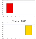
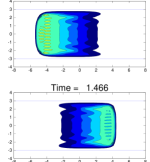
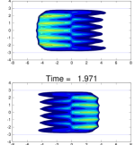
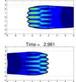
A classical situation considered in the engineering literature is that of two groups of people moving in opposite directions and crossing each other. The numerical integration (see Figure 5), shows formation of lanes that are not superimposing as described in the engineering literature ([14, 10] orย [1] ).

Refer to caption
Refer to caption
Refer to caption
Refer to caption
Figure 5: Numerical integration ofย (12). Above, the population ฯ1subscript๐œŒ1\rho_{1} moving to the right and, below, ฯ2subscript๐œŒ2\rho_{2} moving to the left. Note the lanes that are formed. First, due to the self-interaction (ฮตi=0.3subscript๐œ€๐‘–0.3\varepsilon_{i}=0.3) within each populations and then due to the crossing between the two populations (ฮตo=0.7subscript๐œ€๐‘œ0.7\varepsilon_{o}=0.7). The latter lanes of different populations do not superimpose. Picture from [6].

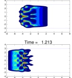
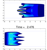
Another situation developping interesting features is the following: two populations are initially uniformly distributed in the same region. At time t =0, the first populations starts moving towards an exit (first line of Figure 6), on the right while the second moves only to let the first one pass (second line of Figure 6).

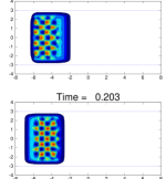
Refer to caption
Refer to caption
Refer to caption
Refer to caption
Figure 6: Numerical integration ofย (12) when with ฮตi=0subscript๐œ€๐‘–0\varepsilon_{i}=0, ฮตo=0.3subscript๐œ€๐‘œ0.3\varepsilon_{o}=0.3. Above, the population ฯ1subscript๐œŒ1\rho_{1} and, below, ฯ2subscript๐œŒ2\rho_{2}. Note first the formation of small clusters separating the two populations, then lanes and, finally, a sort of fingering. Picture from [6].

2.2.3 Interaction group / isolated agent

Let us finally introduce a model that would take into account the situation in which an isolated individual interact with a crowd. We think for example to the situation in which a predator is running after a group of preys. We can also think to the case of a leader willing to carry a group of followers to a given region. Let ฯโˆˆโ„+๐œŒsubscriptโ„\rho\in{\mathbb{R}}_{+} be the density of the group and pโˆˆโ„k๐‘superscriptโ„๐‘˜p\in{\mathbb{R}}^{k} be the position of an isolated agent (e.g. a leader or a predator). We describe the interaction by the coupling (see [7]):

{โˆ‚tฯ+Divโ€‹(ฯโ€‹Vโ€‹(t,x,ฯ,pโ€‹(t)))=0,pห™=ฯ†โ€‹(t,p,(Aโ€‹ฯโ€‹(t))โ€‹(pโ€‹(t))),(t,x)โˆˆโ„+ร—โ„N,casessubscript๐‘ก๐œŒDiv๐œŒ๐‘‰๐‘ก๐‘ฅ๐œŒ๐‘๐‘ก0ห™๐‘๐œ‘๐‘ก๐‘๐ด๐œŒ๐‘ก๐‘๐‘ก๐‘ก๐‘ฅsuperscriptโ„superscriptโ„๐‘\left\{\begin{array}[]{l}\partial_{t}\rho+{\mathrm{Div}}\big{(}\rho\,V\left(t,x,\rho,p(t)\right)\big{)}=0\,,\\ \dot{p}=\varphi\left(t,p,\left(A\rho(t)\right)(p(t))\right)\,,\end{array}\right.\qquad\begin{array}[]{rcl}(t,x)&\in&{\mathbb{R}}^{+}\times{\mathbb{R}}^{N}\,,\end{array} (13)

with initial conditions

ฯโ€‹(0,x)=ฯ0โ€‹(x),pโ€‹(0)=p0.formulae-sequence๐œŒ0๐‘ฅsubscript๐œŒ0๐‘ฅ๐‘0subscript๐‘0\rho(0,x)=\rho_{0}(x)\,,\qquad\qquad p(0)=p_{0}\,.

Using once again Kruลพkov theory and tools on the stability of ordinary differential equations, in collaboration with R. M. Colombo, we proved existence and uniqueness of solutions (see [7, Theorem 2.2]).

For example, we can consider:

  • โ€ข

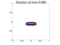
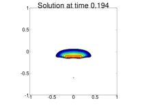
    Followers / Leader (see Figure 7): here the vector pโˆˆโ„2๐‘superscriptโ„2p\in{\mathbb{R}}^{2} is the position of the leader and ฯ๐œŒ\rho is the density of the group of followers. The function vโ€‹(ฯ)๐‘ฃ๐œŒv(\rho) describes essentially the speed of the followers and is, as usual, a decreasing function, vanishing in ฯ=1๐œŒ1\rho=1; the direction of a follower located in x๐‘ฅx is given by the vector pโ€‹(t)โˆ’x๐‘๐‘ก๐‘ฅp(t)-x, directed toward the leader. The velocity of the leader is increasing with respect to the averaged density ฯโˆ—ฮท๐œŒ๐œ‚\rho*\eta, computed in the position of the leader. Indeed, we expect the leader to wait for the followers to join him when the density of followers is small around him, and to accelerate when the density of followers becomes bigger; this means low speed when the averaged density is small and high speed when the averaged density is maximal. The direction of the leader is a chosen vector field ฯˆโ†’โ€‹(t)โ†’๐œ“๐‘ก\vec{\psi}(t).

    {โˆ‚tฯ+Divโ€‹(ฯโ€‹vโ€‹(ฯ)โ€‹(pโ€‹(t)โˆ’x)โ€‹eโˆ’โ€–pโˆ’xโ€–)=0,pห™=(1+ฯโˆ—ฮทโ€‹(pโ€‹(t)))โ€‹ฯˆโ†’โ€‹(t).casessubscript๐‘ก๐œŒDiv๐œŒ๐‘ฃ๐œŒ๐‘๐‘ก๐‘ฅsuperscript๐‘’norm๐‘๐‘ฅ0ห™๐‘1๐œŒ๐œ‚๐‘๐‘กโ†’๐œ“๐‘ก\left\{\begin{array}[]{l}\partial_{t}\rho+{\mathrm{Div}}\left(\rho\,v(\rho)\,(p(t)-x)e^{-{\left\|p-x\right\|}}\right)=0\,,\\[5.0pt] \dot{p}=(1+\rho*\eta(p(t))\,)\;\vec{{\psi}}(t)\,.\end{array}\right.
    Refer to caption
    Refer to caption
    Refer to caption
    Refer to caption
    Refer to caption
    Refer to caption
    Figure 7: Numerical solution of (13) in a predator/prey interaction. Picture from [7].
  • โ€ข

    Sheeps / Dogs: in this example, there are n๐‘›n dogs, located in piโ€‹(t)โˆˆโ„2subscript๐‘๐‘–๐‘กsuperscriptโ„2p_{i}(t)\in{\mathbb{R}}^{2} for iโˆˆ{1,โ€ฆ,n}๐‘–1โ€ฆ๐‘›i\in\{1,\ldots,n\} and a group of sheeps of density ฯโ€‹(t,x)๐œŒ๐‘ก๐‘ฅ\rho(t,x). The dogs want to constrain the sheeps to a given area by running around them and the sheeps are afraid by the dogs. As above, the speed of the sheeps is given by the decreasing function vโ€‹(ฯ)๐‘ฃ๐œŒv(\rho) that vanishes in ฯ=1๐œŒ1\rho=1. The direction of a sheep located in x๐‘ฅx is a sum of two terms. The first one is their prefered direction ฮฝโ†’โ€‹(x)โ†’๐œˆ๐‘ฅ\vec{\nu}(x) ; the second one is given by the vector โˆ‘i=1n(xโˆ’piโ€‹(t))โ€‹eโˆ’โ€–piโˆ’xโ€–superscriptsubscript๐‘–1๐‘›๐‘ฅsubscript๐‘๐‘–๐‘กsuperscript๐‘’normsubscript๐‘๐‘–๐‘ฅ\sum_{i=1}^{n}(x-p_{i}(t))e^{-{\left\|p_{i}-x\right\|}} representing the repulsive effects of the dogs on the sheeps, and its presence is is less felt if it is too far away. Each dog run around the flock tacking the direction perpendicular to the direction of maximal averaged density.

    {โˆ‚tฯ+Divโ€‹(ฯโ€‹vโ€‹(ฯ)โ€‹(ฮฝโ†’โ€‹(x)+โˆ‘i=1n(xโˆ’pi)โ€‹eโˆ’โ€–piโˆ’xโ€–))=0,pห™i=(ฯโˆ—โˆ‡ฮท)โŸ‚โ€‹(piโ€‹(t))1+โ€–ฯโˆ—โˆ‡ฮทโ€‹(piโ€‹(t))โ€–2,for allย โ€‹iโˆˆ{1,โ€ฆโ€‹n}.casessubscript๐‘ก๐œŒDiv๐œŒ๐‘ฃ๐œŒโ†’๐œˆ๐‘ฅsuperscriptsubscript๐‘–1๐‘›๐‘ฅsubscript๐‘๐‘–superscript๐‘’normsubscript๐‘๐‘–๐‘ฅ0formulae-sequencesubscriptห™๐‘๐‘–superscript๐œŒโˆ‡๐œ‚perpendicular-tosubscript๐‘๐‘–๐‘ก1superscriptnorm๐œŒโˆ‡๐œ‚subscript๐‘๐‘–๐‘ก2for allย ๐‘–1โ€ฆ๐‘›\left\{\begin{array}[]{l}\partial_{t}\rho+{\mathrm{Div}}\left(\rho\,v(\rho)\left(\vec{\nu}(x)+\sum_{i=1}^{n}(x-p_{i})e^{-{\left\|p_{i}-x\right\|}}\right)\right)=0\,,\\[5.0pt] \displaystyle\dot{p}_{i}=\frac{(\rho*\nabla\eta)^{\perp}(p_{i}(t))}{\sqrt{1+{\left\|\rho*\nabla\eta(p_{i}(t))\right\|}^{2}}}\,,\qquad\textrm{for all }i\in\{1,\ldots n\}\,.\end{array}\right.
  • โ€ข

    Preys / Predator: here a predator, located in pโ€‹(t)โˆˆโ„3๐‘๐‘กsuperscriptโ„3p(t)\in{\mathbb{R}}^{3} is pursuing a group of preys of density ฯโ€‹(t,x)๐œŒ๐‘ก๐‘ฅ\rho(t,x). For example, we can think to an hawk pursuing a swarm of little birds or to a shark pursuing a shoal of little fishes. As above, the speed of the preys is given by the decreasing function vโ€‹(ฯ)๐‘ฃ๐œŒv(\rho) that vanishes in ฯ=1๐œŒ1\rho=1. The direction of a prey located in x๐‘ฅx is given by the vector (xโˆ’pโ€‹(t))โ€‹eโˆ’โ€–pโ€‹(t)โˆ’xโ€–๐‘ฅ๐‘๐‘กsuperscript๐‘’norm๐‘๐‘ก๐‘ฅ(x-p(t))e^{-{\left\|p(t)-x\right\|}} so that the predator has a repulsive effect on the preys, and its presence is is less felt if it is too far away. The acceleration of the predator is directed toward the maximal averaged density of preys, as felt from its position, so it is directed as โˆ‡(ฯโˆ—ฮท)โก(pโ€‹(t))โˆ‡๐œŒ๐œ‚๐‘๐‘ก\nabla(\rho*\eta)(p(t)).

    {โˆ‚tฯ+Divโ€‹(ฯโ€‹vโ€‹(ฯ)โ€‹(1+eโˆ’โ€–xโˆ’pโ€‹(t)โ€–โ€‹(xโˆ’pโ€‹(t))))=0,d2โ€‹pdโ€‹t2=(ฯโˆ—โˆ‡)โ€‹ฮทโ€‹(pโ€‹(t)).casessubscript๐‘ก๐œŒDiv๐œŒ๐‘ฃ๐œŒ1superscript๐‘’norm๐‘ฅ๐‘๐‘ก๐‘ฅ๐‘๐‘ก0superscriptd2๐‘dsuperscript๐‘ก2๐œŒโˆ‡๐œ‚๐‘๐‘ก\left\{\begin{array}[]{l}\partial_{t}\rho+{\mathrm{Div}}\left(\rho\,v(\rho)\,\left(1+\,e^{-{\left\|x-p(t)\right\|}}\,\left(x-p(t)\right)\right)\right)=0\,,\\[5.0pt] \displaystyle\frac{\mathrm{d}^{2}p}{\mathrm{d}t^{2}}=(\rho*\nabla)\eta(p(t))\,.\end{array}\right.

Note that Theorem 2.6 deals with measure solutions. Consequently, if ฯ1โˆˆ๐‹๐Ÿsubscript๐œŒ1superscript๐‹1\rho_{1}\in\mathbf{L^{1}} and ฯ2=ฮดpโ€‹(t)subscript๐œŒ2subscript๐›ฟ๐‘๐‘ก\rho_{2}=\delta_{p(t)}, we recover the above coupling PDE/ODE. However, in Theorem 2.6, there are restricitions on the flow as we only deal with continuity equations. In particular, with a well-chosen nonlinearity with respect to ฯ๐œŒ\rho in the first equation of (13), we are able to provide for (13) an a priori uniform bound on the ๐‹โˆžsuperscript๐‹\mathbf{L^{\infty}} norm, which is not possible for (10): in the three examples above, if vโ€‹(1)=0๐‘ฃ10v(1)=0, then 0โ‰คฯ0โ‰ค10subscript๐œŒ010\leq\rho_{0}\leq 1 implies 0โ‰คฯโ€‹(t)โ‰ค10๐œŒ๐‘ก10\leq\rho(t)\leq 1 for all tโ‰ฅ0๐‘ก0t\geq 0.

3 Using Kruลพkov theory

3.1 General Theory on scalar conservation laws

In this section, we consider classical scalar conservation laws.

โˆ‚tu+Divโ€‹fโ€‹(t,x,u)=Fโ€‹(t,x,u),uโ€‹(0,x)=u0โ€‹(x),formulae-sequencesubscript๐‘ก๐‘ขDiv๐‘“๐‘ก๐‘ฅ๐‘ข๐น๐‘ก๐‘ฅ๐‘ข๐‘ข0๐‘ฅsubscript๐‘ข0๐‘ฅ\partial_{t}u+{\mathrm{Div}}f(t,x,u)=F(t,x,u)\,,\qquad\qquad u(0,x)=u_{0}(x)\,, (14)

where f๐‘“f is the flow and F๐นF is the source. Note that, DivDiv{\mathrm{Div}} stands for the total divergence whereas divdiv{\mathrm{div}} stands for the partial divergence. Thus Divโ€‹fโ€‹(t,x,uโ€‹(t,x))=divโ€‹fโ€‹(t,x,uโ€‹(t,x))+โˆ‚ufโ€‹(t,x,uโ€‹(t,x))โ‹…โˆ‡uโ€‹(t,x)Div๐‘“๐‘ก๐‘ฅ๐‘ข๐‘ก๐‘ฅdiv๐‘“๐‘ก๐‘ฅ๐‘ข๐‘ก๐‘ฅsubscript๐‘ขโ‹…๐‘“๐‘ก๐‘ฅ๐‘ข๐‘ก๐‘ฅโˆ‡๐‘ข๐‘ก๐‘ฅ{\mathrm{Div}}f(t,x,u(t,x))={\mathrm{div}}f(t,x,u(t,x))+\partial_{u}f(t,x,u(t,x))\cdot\nabla u(t,x).

Let us recall the definition of weak entropy solution:

Definition 3.1.

The function ฯโˆˆ๐‹โˆžโ€‹([0,T]ร—โ„N,โ„)๐œŒsuperscript๐‹0๐‘‡superscriptโ„๐‘โ„\rho\in\mathbf{L^{\infty}}([0,T]\times{\mathbb{R}}^{N},{\mathbb{R}}) is called weak entropy solution to the Cauchy problem (14) if it satisfies for all kโˆˆโ„๐‘˜โ„k\in{\mathbb{R}} and any test-function ฯ†โˆˆ๐’žc0(]โˆ’โˆž,T[ร—โ„N,โ„+)\varphi\in\mathscr{C}_{c}^{0}(]-\infty,T[\times{\mathbb{R}}^{N},{\mathbb{R}}_{+}),

โˆซโ„+โˆ—โˆซโ„N[(uโˆ’k)โ€‹โˆ‚tฯ†+(fโ€‹(t,x,u)โˆ’fโ€‹(t,x,k))โ€‹โˆ‡xฯ†+(Fโ€‹(t,x,u)โˆ’divโ€‹fโ€‹(t,x,k))โ€‹ฯ†]ร—sign(uโˆ’k)dxdt+โˆซโ„N|ฯ0(x)โˆ’k|ฯ†(0,x)dโ€‹xโ‰ฅ0.\begin{array}[]{r}\displaystyle\int_{{\mathbb{R}}_{+}^{*}}\int_{{\mathbb{R}}^{N}}\left[(u-k)\,\partial_{t}\varphi+\left(f(t,x,u)-f(t,x,k)\right)\nabla_{x}\varphi+\left(F(t,x,u)-{\mathrm{div}}f(t,x,k)\right)\varphi\right]\\ \times\mathrm{sign}(u-k)\,\mathrm{d}x\,\mathrm{d}t+\int_{{\mathbb{R}}^{N}}{\left|\rho_{0}(x)-k\right|}\varphi(0,x)\mathinner{\mathrm{d}{x}}\geq 0\,.\end{array} (15)

We also recall the well-known Kruลพkov theorem [17, Theorem 4], giving existence and uniqueness of weak entropy solutions.

Theorem 3.2 (Kruลพkov).

Let u0โˆˆ(๐‹โˆžโˆฉ๐‹๐Ÿ)โ€‹(โ„N,โ„)subscript๐‘ข0superscript๐‹superscript๐‹1superscriptโ„๐‘โ„u_{0}\in(\mathbf{L^{\infty}}\cap\mathbf{L^{1}})({\mathbb{R}}^{N},{\mathbb{R}}). For all A,Tโ‰ฅ0๐ด๐‘‡0A,T\geq 0, we denote ฮฉTA=[0,T]ร—โ„Nร—[โˆ’A,A]superscriptsubscriptฮฉ๐‘‡๐ด0๐‘‡superscriptโ„๐‘๐ด๐ด\Omega_{T}^{A}=[0,T]\times{\mathbb{R}}^{N}\times[-A,A] and ฮฉ=โ„+ร—โ„Nร—โ„ฮฉsubscriptโ„superscriptโ„๐‘โ„\Omega={\mathbb{R}}_{+}\times{\mathbb{R}}^{N}\times{\mathbb{R}}. Under the conditions fโˆˆ๐’ž0โ€‹(ฮฉ;โ„N)๐‘“superscript๐’ž0ฮฉsuperscriptโ„๐‘f\in\mathscr{C}^{0}(\Omega;{\mathbb{R}}^{N}), Fโˆˆ๐’ž0โ€‹(ฮฉ;โ„)๐นsuperscript๐’ž0ฮฉโ„F\in\mathscr{C}^{0}(\Omega;{\mathbb{R}}) and

(๐Š){fโˆˆ๐’ž0โ€‹(ฮฉ;โ„N),Fโˆˆ๐’ž0โ€‹(ฮฉ;โ„),ย and for allย โ€‹T,A>0:f,Fโ€‹ย have continuous derivatives:ย โ€‹โˆ‚uf,โˆ‚uโˆ‡f,โˆ‡2f,โˆ‚uF,โˆ‡F,for allย โ€‹T,A>0,โˆ‚ufโˆˆ๐‹โˆžโ€‹(ฮฉTA),Fโˆ’divโ€‹fโˆˆ๐‹โˆžโ€‹(ฮฉTA),โˆ‚u(Fโˆ’divโ€‹f)โˆˆ๐‹โˆžโ€‹(ฮฉTA)๐Šcases:formulae-sequence๐‘“superscript๐’ž0ฮฉsuperscriptโ„๐‘formulae-sequence๐นsuperscript๐’ž0ฮฉโ„ย and for allย ๐‘‡๐ด0absent๐‘“๐นย have continuous derivatives:ย subscript๐‘ข๐‘“subscript๐‘ขโˆ‡๐‘“superscriptโˆ‡2๐‘“subscript๐‘ข๐นโˆ‡๐นformulae-sequencefor allย ๐‘‡๐ด0subscript๐‘ข๐‘“superscript๐‹superscriptsubscriptฮฉ๐‘‡๐ดformulae-sequence๐นdiv๐‘“superscript๐‹superscriptsubscriptฮฉ๐‘‡๐ดsubscript๐‘ข๐นdiv๐‘“superscript๐‹superscriptsubscriptฮฉ๐‘‡๐ด\begin{array}[]{cl}\mathbf{(K)}&\left\{\begin{array}[]{l}f\in\mathscr{C}^{0}(\Omega;{\mathbb{R}}^{N})\,,\qquad F\in\mathscr{C}^{0}(\Omega;{\mathbb{R}})\,,\textrm{ and for all }T,A>0:\\[5.0pt] f\,,\;F\;\textrm{ have continuous derivatives: }\;\partial_{u}f\,,\;\partial_{u}\nabla f\,,\;\nabla^{2}f\,,\;\partial_{u}F\,,\;\nabla F\,,\\ \textrm{for all }T,A>0\;,\;\;\partial_{u}f\in\mathbf{L^{\infty}}(\Omega_{T}^{A})\,,\\ F-{\mathrm{div}}f\in\mathbf{L^{\infty}}(\Omega_{T}^{A})\,,\qquad\;\partial_{u}(F-{\mathrm{div}}f)\in\mathbf{L^{\infty}}(\Omega_{T}^{A})\end{array}\right.\end{array}

there exists a unique weak entropy solution uโˆˆ๐‹โˆžโ€‹([0,T];๐‹๐Ÿโ€‹(โ„N;โ„))๐‘ขsuperscript๐‹0๐‘‡superscript๐‹1superscriptโ„๐‘โ„u\in\mathbf{L^{\infty}}([0,T];\mathbf{L^{1}}({\mathbb{R}}^{N};{\mathbb{R}})) of (14) that is right-continuous in time.

Let v0โˆˆ(๐‹๐Ÿโˆฉ๐‹โˆž)โ€‹(โ„N;โ„)subscript๐‘ฃ0superscript๐‹1superscript๐‹superscriptโ„๐‘โ„v_{0}\in(\mathbf{L^{1}}\cap\mathbf{L^{\infty}})({\mathbb{R}}^{N};{\mathbb{R}}). Let u๐‘ขu be the solution associated to the initial condition u0subscript๐‘ข0u_{0} and v๐‘ฃv be the solution associated to the initial condition v0subscript๐‘ฃ0v_{0}. Let M๐‘€M be such that Mโ‰ฅsup(โ€–uโ€–๐‹โˆžโ€‹(โ„+ร—โ„N;โ„),โ€–vโ€–๐‹โˆžโ€‹([0,T]ร—โ„N;โ„))๐‘€supremumsubscriptnorm๐‘ขsuperscript๐‹subscriptโ„superscriptโ„๐‘โ„subscriptnorm๐‘ฃsuperscript๐‹0๐‘‡superscriptโ„๐‘โ„M\geq\sup({\left\|u\right\|}_{\mathbf{L^{\infty}}({\mathbb{R}}_{+}\times{\mathbb{R}}^{N};{\mathbb{R}})},{\left\|v\right\|}_{\mathbf{L^{\infty}}([0,T]\times{\mathbb{R}}^{N};{\mathbb{R}})}). Then, for all tโˆˆ[0,T]๐‘ก0๐‘‡t\in[0,T], with ฮณ=โ€–โˆ‚uFโ€–๐‹โˆžโ€‹(ฮฉTM)๐›พsubscriptnormsubscript๐‘ข๐นsuperscript๐‹superscriptsubscriptฮฉ๐‘‡๐‘€\gamma={\left\|\partial_{u}F\right\|}_{\mathbf{L^{\infty}}(\Omega_{T}^{M})}, we have

โ€–(uโˆ’v)โ€‹(t)โ€–๐‹๐Ÿโ‰คeฮณโ€‹tโ€‹โ€–u0โˆ’v0โ€–๐‹๐Ÿ.subscriptnorm๐‘ข๐‘ฃ๐‘กsuperscript๐‹1superscript๐‘’๐›พ๐‘กsubscriptnormsubscript๐‘ข0subscript๐‘ฃ0superscript๐‹1{\left\|{(u-v)(t)}\right\|}_{\mathbf{L^{1}}}\leq e^{\gamma t}{\left\|u_{0}-v_{0}\right\|}_{\mathbf{L^{1}}}\,. (16)

3.1.1 Estimate on the dependence with respect to flow and source

Let us now consider a pair of different flows f,gโˆˆ๐’ž2โ€‹([0,T]ร—โ„Nร—โ„;โ„N)๐‘“๐‘”superscript๐’ž20๐‘‡superscriptโ„๐‘โ„superscriptโ„๐‘f,g\in\mathscr{C}^{2}([0,T]\times{\mathbb{R}}^{N}\times{\mathbb{R}};{\mathbb{R}}^{N}) and different sources F,Gโˆˆ๐’ž1โ€‹([0,T]ร—โ„Nร—โ„;โ„)๐น๐บsuperscript๐’ž10๐‘‡superscriptโ„๐‘โ„โ„F,G\in\mathscr{C}^{1}([0,T]\times{\mathbb{R}}^{N}\times{\mathbb{R}};{\mathbb{R}}), let us denote u,v๐‘ข๐‘ฃu,v the solutions of

โˆ‚tu+Divโ€‹fโ€‹(t,x,u)subscript๐‘ก๐‘ขDiv๐‘“๐‘ก๐‘ฅ๐‘ข\displaystyle\partial_{t}u+{\mathrm{Div}}\,f(t,x,u) =Fโ€‹(t,x,u),absent๐น๐‘ก๐‘ฅ๐‘ข\displaystyle=F(t,x,u)\,, uโ€‹(0,โ‹…)๐‘ข0โ‹…\displaystyle u(0,\cdot) =u0,absentsubscript๐‘ข0\displaystyle=u_{0}\,, (17)
โˆ‚tv+Divโ€‹gโ€‹(t,x,v)subscript๐‘ก๐‘ฃDiv๐‘”๐‘ก๐‘ฅ๐‘ฃ\displaystyle\partial_{t}v+{\mathrm{Div}}\,g(t,x,v) =Gโ€‹(t,x,v),absent๐บ๐‘ก๐‘ฅ๐‘ฃ\displaystyle=G(t,x,v)\,, vโ€‹(0,โ‹…)๐‘ฃ0โ‹…\displaystyle v(0,\cdot) =v0,absentsubscript๐‘ฃ0\displaystyle=v_{0}\,, (18)

with initial conditions u0,v0โˆˆ(๐‹๐Ÿโˆฉ๐‹โˆžโˆฉ๐๐•)โ€‹(โ„N,โ„)subscript๐‘ข0subscript๐‘ฃ0superscript๐‹1superscript๐‹๐๐•superscriptโ„๐‘โ„u_{0},v_{0}\in(\mathbf{L^{1}}\cap\mathbf{L^{\infty}}\cap\mathbf{BV})({\mathbb{R}}^{N},{\mathbb{R}}). We want here to estimate โ€–(uโˆ’v)โ€‹(t)โ€–๐‹๐Ÿsubscriptnorm๐‘ข๐‘ฃ๐‘กsuperscript๐‹1{\left\|(u-v)(t)\right\|}_{\mathbf{L^{1}}} with fโˆ’g๐‘“๐‘”f-g, Fโˆ’G๐น๐บF-G, u0โˆ’v0subscript๐‘ข0subscript๐‘ฃ0u_{0}-v_{0}. To do that, we use the doubling variable method due to Kruลพkov [17]. This strategy was already employed by Lucier [19] and Bouchut & Perthame [3] to study the case in which the flows f,g๐‘“๐‘”f,g depend only on u๐‘ขu and the source are identically zero (F=G=0๐น๐บ0F=G=0). A key ingredient in the previous results is that the solution of โˆ‚tu+Divโ€‹(fโ€‹(u))=0subscript๐‘ก๐‘ขDiv๐‘“๐‘ข0\partial_{t}u+{\mathrm{Div}}(f(u))=0 with initial condition u0โˆˆ(๐‹โˆžโˆฉ๐‹๐Ÿโˆฉ๐๐•)โ€‹(โ„N,โ„)subscript๐‘ข0superscript๐‹superscript๐‹1๐๐•superscriptโ„๐‘โ„u_{0}\in(\mathbf{L^{\infty}}\cap\mathbf{L^{1}}\cap\mathbf{BV})({\mathbb{R}}^{N},{\mathbb{R}}) satisfies TVโ€‹(uโ€‹(t))โ‰คTVโ€‹(u0)TV๐‘ข๐‘กTVsubscript๐‘ข0\mathrm{TV}(u(t))\leq\mathrm{TV}(u_{0}).

Let us remind the definition of total variation.

Definition 3.3.

For uโˆˆ๐‹๐ฅ๐จ๐œ๐Ÿโ€‹(โ„N;โ„)๐‘ขsubscriptsuperscript๐‹1๐ฅ๐จ๐œsuperscriptโ„๐‘โ„u\in\mathbf{L^{1}_{loc}}({\mathbb{R}}^{N};{\mathbb{R}}) we denote the total variation ofย u๐‘ขu:

TVโ€‹(u)TV๐‘ข\displaystyle\mathrm{TV}(u) =\displaystyle= sup{โˆซโ„Nudivฮจ;ฮจโˆˆ๐’žc1(โ„N;โ„N),โˆฅฮจโˆฅ๐‹โˆžโ‰ค1}.\displaystyle\mathrm{sup}\big{\{}\int_{{\mathbb{R}}^{N}}u\,{\mathrm{div}}\Psi\,;\quad\Psi\in\mathscr{C}_{c}^{1}({\mathbb{R}}^{N};{\mathbb{R}}^{N})\,,\quad{\left\|\Psi\right\|}_{\mathbf{L^{\infty}}}\leq 1\big{\}}\,.

The space of function with bounded variation is then defined as

๐๐•โ€‹(โ„N;โ„)={uโˆˆ๐‹๐ฅ๐จ๐œ๐Ÿ;TVโ€‹(u)<โˆž}.๐๐•superscriptโ„๐‘โ„formulae-sequence๐‘ขsubscriptsuperscript๐‹1๐ฅ๐จ๐œTV๐‘ข\mathbf{BV}({\mathbb{R}}^{N};{\mathbb{R}})=\left\{u\in\mathbf{L^{1}_{loc}};\mathrm{TV}(u)<\infty\right\}\,.
Remark 3.4.

If uโˆˆ(๐’ž1โˆฉ๐–๐Ÿ,๐Ÿ)โ€‹(โ„N,โ„)๐‘ขsuperscript๐’ž1superscript๐–11superscriptโ„๐‘โ„u\in(\mathscr{C}^{1}\cap\mathbf{W^{1,1}})({\mathbb{R}}^{N},{\mathbb{R}}) then TVโ€‹(u)=โ€–โˆ‡uโ€–๐‹๐ŸTV๐‘ขsubscriptnormโˆ‡๐‘ขsuperscript๐‹1\mathrm{TV}(u)={\left\|\nabla u\right\|}_{\mathbf{L^{1}}}. When f๐‘“f and F๐นF are not depending on u๐‘ขu, we have

u0โˆˆ(๐‹โˆžโˆฉ๐๐•)โ€‹(โ„N,โ„)โ‡’โˆ€tโ‰ฅ0,uโ€‹(t)โˆˆ(๐‹โˆžโˆฉ๐๐•)โ€‹(โ„N,โ„)formulae-sequencesubscript๐‘ข0superscript๐‹๐๐•superscriptโ„๐‘โ„โ‡’for-all๐‘ก0๐‘ข๐‘กsuperscript๐‹๐๐•superscriptโ„๐‘โ„u_{0}\in(\mathbf{L^{\infty}}\cap\mathbf{BV})({\mathbb{R}}^{N},{\mathbb{R}})\Rightarrow\forall t\geq 0\,,\quad u(t)\in(\mathbf{L^{\infty}}\cap\mathbf{BV})({\mathbb{R}}^{N},{\mathbb{R}})

and, with ฮณ=โ€–โˆ‚uFโ€–๐‹โˆžโ€‹(ฮฉTM)๐›พsubscriptnormsubscript๐‘ข๐นsuperscript๐‹superscriptsubscriptฮฉ๐‘‡๐‘€\gamma={\left\|\partial_{u}F\right\|}_{\mathbf{L^{\infty}}(\Omega_{T}^{M})},

TVโ€‹(uโ€‹(t))โ‰คTVโ€‹(u0)โ€‹eฮณโ€‹t.TV๐‘ข๐‘กTVsubscript๐‘ข0superscript๐‘’๐›พ๐‘ก\mathrm{TV}(u(t))\leq\mathrm{TV}(u_{0})e^{\gamma t}\,.
Theorem 3.5 (see [19]).

Let f,g:โ„โ†’โ„N:๐‘“๐‘”โ†’โ„superscriptโ„๐‘f,g:{\mathbb{R}}\to{\mathbb{R}}^{N} be globally Lipschitz, let u0,v0โˆˆ(๐‹๐Ÿโˆฉ๐‹โˆž)โ€‹(โ„N;โ„)subscript๐‘ข0subscript๐‘ฃ0superscript๐‹1superscript๐‹superscriptโ„๐‘โ„u_{0},v_{0}\in(\mathbf{L^{1}}\cap\mathbf{L^{\infty}})({\mathbb{R}}^{N};{\mathbb{R}}) be initial conditions of

โˆ‚tu+Divโ€‹fโ€‹(u)=0,โˆ‚tv+Divโ€‹gโ€‹(v)=0.formulae-sequencesubscript๐‘ก๐‘ขDiv๐‘“๐‘ข0subscript๐‘ก๐‘ฃDiv๐‘”๐‘ฃ0\partial_{t}u+{\mathrm{Div}}\,f(u)=0\,,\qquad\partial_{t}v+{\mathrm{Div}}\,g(v)=0\,.

Assume furthermore that v0โˆˆ๐๐•โ€‹(โ„N;โ„)subscript๐‘ฃ0๐๐•superscriptโ„๐‘โ„v_{0}\in\mathbf{BV}({\mathbb{R}}^{N};{\mathbb{R}}). Then for all tโ‰ฅ0๐‘ก0t\geq 0,

โ€–(uโˆ’v)โ€‹(t)โ€–๐‹๐Ÿโ‰คโ€–u0โˆ’v0โ€–๐‹๐Ÿ+Cโ€‹tโ€‹TVโ€‹(v0)โ€‹missingโ€‹Lโ€‹iโ€‹pโ€‹(fโˆ’g),subscriptnorm๐‘ข๐‘ฃ๐‘กsuperscript๐‹1subscriptnormsubscript๐‘ข0subscript๐‘ฃ0superscript๐‹1๐ถ๐‘กTVsubscript๐‘ฃ0missing๐ฟ๐‘–๐‘๐‘“๐‘”{\left\|(u-v)(t)\right\|}_{\mathbf{L^{1}}}\leq{\left\|u_{0}-v_{0}\right\|}_{\mathbf{L^{1}}}+C\,t\,\mathrm{TV}(v_{0})\,\mathinner{\mathbf{missing}}{Lip}(f-g)\,,

where C>0๐ถ0C>0 is a given constant.

We want to generalize this theorem. Let us introduce the set of hypotheses:

(๐…๐’)๐…๐’\displaystyle\mathbf{(FS)} {for allย โ€‹U,T>0,โˆ‚uFโˆˆ๐‹โˆžโ€‹(ฮฉTU)โˆซ0Tโˆซโ„Nโ€–(Fโˆ’divโ€‹f)โ€‹(t,x,โ‹…)โ€–๐‹โˆžโ€‹([โˆ’U,U];โ„)โ€‹dxโ€‹dt<+โˆž.casesformulae-sequencefor allย ๐‘ˆ๐‘‡0subscript๐‘ข๐นsuperscript๐‹superscriptsubscriptฮฉ๐‘‡๐‘ˆsuperscriptsubscript0๐‘‡subscriptsuperscriptโ„๐‘subscriptnorm๐นdiv๐‘“๐‘ก๐‘ฅโ‹…superscript๐‹๐‘ˆ๐‘ˆโ„differential-d๐‘ฅdifferential-d๐‘ก\displaystyle\left\{\begin{array}[]{l}\textrm{for all }U,\,T>0\,,\qquad\partial_{u}F\in\mathbf{L^{\infty}}(\Omega_{T}^{U})\\[5.0pt] \displaystyle\int_{0}^{T}\!\!\int_{{\mathbb{R}}^{N}}\!{\left\|(F-{\mathrm{div}}\,f)(t,x,\cdot)\right\|}_{\mathbf{L^{\infty}}({[-U,U]};{\mathbb{R}})}\,\mathrm{d}x\,\mathrm{d}t<+\infty\,.\end{array}\right.

Denoting ฮฉTV=[0,T]ร—โ„Nร—[โˆ’V,V]superscriptsubscriptฮฉ๐‘‡๐‘‰0๐‘‡superscriptโ„๐‘๐‘‰๐‘‰\Omega_{T}^{V}=[0,T]\times{\mathbb{R}}^{N}\times[-V,V], we obtain:

Theorem 3.6 (see [18]).

Assume that (f,F),(g,G)๐‘“๐น๐‘”๐บ(f,F),(g,G) satisfy (K), that (fโˆ’g,Fโˆ’G)๐‘“๐‘”๐น๐บ(f-g,F-G) satisfies (FS). Let u0,v0โˆˆ(๐‹๐Ÿโˆฉ๐‹โˆžโˆฉ๐๐•)โ€‹(โ„N;โ„)subscript๐‘ข0subscript๐‘ฃ0superscript๐‹1superscript๐‹๐๐•superscriptโ„๐‘โ„u_{0},v_{0}\in(\mathbf{L^{1}}\cap\mathbf{L^{\infty}}\cap\mathbf{BV})({\mathbb{R}}^{N};{\mathbb{R}}). Let u๐‘ขu and v๐‘ฃv be the solutions of (17) and (18) associated to (f,F)๐‘“๐น(f,F) and (g,G)๐‘”๐บ(g,G) with initial conditions u0subscript๐‘ข0u_{0} and v0subscript๐‘ฃ0v_{0}. Assume furthermore that TVโ€‹(uโ€‹(t))<โˆžTV๐‘ข๐‘ก\mathrm{TV}(u(t))<\infty for all tโ‰ฅ0๐‘ก0t\geq 0.

Let V=maxโก(โ€–uโ€–๐‹โˆž,โ€–vโ€–๐‹โˆž)๐‘‰subscriptnorm๐‘ขsuperscript๐‹subscriptnorm๐‘ฃsuperscript๐‹V=\max({\left\|u\right\|}_{\mathbf{L^{\infty}}},{\left\|v\right\|}_{\mathbf{L^{\infty}}}) and ฮบ=โ€–โˆ‚uFโ€–๐‹โˆžโ€‹(ฮฉTV)๐œ…subscriptnormsubscript๐‘ข๐นsuperscript๐‹superscriptsubscriptฮฉ๐‘‡๐‘‰\kappa={\left\|\partial_{u}F\right\|}_{\mathbf{L^{\infty}}(\Omega_{T}^{V})}. Then for all tโˆˆ[0,T]๐‘ก0๐‘‡t\in[0,T]:

โ€–(uโˆ’v)โ€‹(t)โ€–๐‹๐Ÿโ‰คeฮบโ€‹tโ€‹โ€–u0โˆ’v0โ€–๐‹๐Ÿ+eฮบโ€‹tโ€‹supฯ„โˆˆ[0,t](TVโ€‹(uโ€‹(ฯ„)))โ€‹โˆซ0tโ€–โˆ‚u(fโˆ’g)โ€‹(ฯ„)โ€–๐‹โˆžโ€‹(โ„Nร—[โˆ’V;V])โ€‹dโ€‹ฯ„subscriptnorm๐‘ข๐‘ฃ๐‘กsuperscript๐‹1superscript๐‘’๐œ…๐‘กsubscriptnormsubscript๐‘ข0subscript๐‘ฃ0superscript๐‹1superscript๐‘’๐œ…๐‘กsubscriptsupremum๐œ0๐‘กTV๐‘ข๐œsuperscriptsubscript0๐‘กsubscriptnormsubscript๐‘ข๐‘“๐‘”๐œsuperscript๐‹superscriptโ„๐‘๐‘‰๐‘‰d๐œ\displaystyle{\left\|(u-v)(t)\right\|}_{\mathbf{L^{1}}}\leq e^{\kappa t}{\left\|u_{0}-v_{0}\right\|}_{\mathbf{L^{1}}}+e^{\kappa t}\sup_{\tau\in[0,t]}\left(\mathrm{TV}(u(\tau))\right)\int_{0}^{t}{\left\|\partial_{u}(f-g)(\tau)\right\|}_{\mathbf{L^{\infty}}({\mathbb{R}}^{N}\times[-V;V])}\mathinner{\mathrm{d}{\tau}}
+โˆซ0teฮบโ€‹(tโˆ’ฯ„)โ€‹โˆซโ„Nโ€–((Fโˆ’G)โˆ’divโ€‹(fโˆ’g))โ€‹(ฯ„,x,โ‹…)โ€–๐‹โˆžโ€‹([โˆ’V,V])โ€‹dxโ€‹dฯ„.superscriptsubscript0๐‘กsuperscript๐‘’๐œ…๐‘ก๐œsubscriptsuperscriptโ„๐‘subscriptnorm๐น๐บdiv๐‘“๐‘”๐œ๐‘ฅโ‹…superscript๐‹๐‘‰๐‘‰differential-d๐‘ฅdifferential-d๐œ\displaystyle\quad+\int_{0}^{t}e^{\kappa(t-\tau)}\int_{{\mathbb{R}}^{N}}{\left\|((F-G)-{\mathrm{div}}\,(f-g))(\tau,x,\cdot)\right\|}_{\mathbf{L^{\infty}}({[-V,V]})}\mathrm{d}x\mathrm{d}\tau\,.

The proof of this theorem is based on the Kruลพkov doubling variables method and is detailed in [18].

In some particular cases, we recover known estimates:

  • โ€ข

    fโ€‹(u),gโ€‹(u),F=G=0๐‘“๐‘ข๐‘”๐‘ข๐น๐บ0f(u),g(u),F=G=0 : ฮบ=0๐œ…0\kappa=0 and

    โ€–(uโˆ’v)โ€‹(t)โ€–๐‹๐Ÿโ‰คโ€–u0โˆ’v0โ€–๐‹๐Ÿ+tโ€‹TVโ€‹(u0)โ€‹โ€–โˆ‚u(fโˆ’g)โ€–๐‹โˆžโ€‹(ฮฉTV).subscriptnorm๐‘ข๐‘ฃ๐‘กsuperscript๐‹1subscriptnormsubscript๐‘ข0subscript๐‘ฃ0superscript๐‹1๐‘กTVsubscript๐‘ข0subscriptnormsubscript๐‘ข๐‘“๐‘”superscript๐‹superscriptsubscriptฮฉ๐‘‡๐‘‰\displaystyle{\left\|(u-v)(t)\right\|}_{\mathbf{L^{1}}}\leq{\left\|u_{0}-v_{0}\right\|}_{\mathbf{L^{1}}}+t\,\mathrm{TV}(u_{0}){\left\|\partial_{u}(f-g)\right\|}_{\mathbf{L^{\infty}}({\Omega_{T}^{V}})}\,.
  • โ€ข

    fโ€‹(t,x),Fโ€‹(t,x)๐‘“๐‘ก๐‘ฅ๐น๐‘ก๐‘ฅf(t,x),F(t,x) : ฮบ=0๐œ…0\kappa=0, uโ€‹(t,x)=u0โ€‹(x)+โˆซ0t(Fโˆ’divโ€‹f)โ€‹(ฯ„,x)โ€‹dโ€‹ฯ„๐‘ข๐‘ก๐‘ฅsubscript๐‘ข0๐‘ฅsuperscriptsubscript0๐‘ก๐นdiv๐‘“๐œ๐‘ฅd๐œu(t,x)=u_{0}(x)+\int_{0}^{t}(F-{\mathrm{div}}f)(\tau,x)\mathinner{\mathrm{d}{\tau}}, and

    โ€–(uโˆ’v)โ€‹(t)โ€–๐‹๐Ÿโ‰คsubscriptnorm๐‘ข๐‘ฃ๐‘กsuperscript๐‹1absent\displaystyle{\left\|(u-v)(t)\right\|}_{\mathbf{L^{1}}}\leq โ€–u0โˆ’v0โ€–๐‹๐Ÿ+โˆซ0tโˆซโ„N|((Fโˆ’G)โˆ’divโ€‹(fโˆ’g))โ€‹(ฯ„,x)|โ€‹dxโ€‹dฯ„.subscriptnormsubscript๐‘ข0subscript๐‘ฃ0superscript๐‹1superscriptsubscript0๐‘กsubscriptsuperscriptโ„๐‘๐น๐บdiv๐‘“๐‘”๐œ๐‘ฅdifferential-d๐‘ฅdifferential-d๐œ\displaystyle{\left\|u_{0}-v_{0}\right\|}_{\mathbf{L^{1}}}+\int_{0}^{t}\int_{{\mathbb{R}}^{N}}{\left|((F-G)-{\mathrm{div}}\,(f-g))(\tau,x)\right|}\mathrm{d}x\mathrm{d}\tau\,.

3.1.2 Total variation estimate

To complete Theorem 3.6, we need an estimate on the total variation, defined in Definition 3.3. To do so we need a few more hypotheses. Indeed, there is no reason why the total variation should be bounded for all time. In fact, let us consider the equation โˆ‚tu+โˆ‚xcosโกx=0subscript๐‘ก๐‘ขsubscript๐‘ฅ๐‘ฅ0\partial_{t}u+\partial_{x}\cos x=0, u0=0subscript๐‘ข00u_{0}=0. The solution of this Cauchy problem is uโ€‹(t,x)=tโ€‹sinโกx๐‘ข๐‘ก๐‘ฅ๐‘ก๐‘ฅu(t,x)=t\sin x whose total variation is 0 at time 0 and +โˆž+\infty for any time t>0๐‘ก0t>0.

Our goal now is to give a general estimate on the total variation. Let us introduce the following set of hypotheses

(๐“๐•):{for allย โ€‹A,T>0โˆ‡โ€‹โˆ‚ufโˆˆ๐‹โˆžโ€‹(ฮฉTA;โ„Nร—N),โˆ‚uFโˆˆ๐‹โˆžโ€‹(ฮฉTA;โ„),โˆซ0Tโˆซโ„Nโ€–โˆ‡(Fโˆ’divโ€‹f)โก(t,x,โ‹…)โ€–๐‹โˆžโ€‹([โˆ’A,A];โ„N)<โˆž.:๐“๐•casesfor allย ๐ด๐‘‡0formulae-sequenceโˆ‡subscript๐‘ข๐‘“superscript๐‹superscriptsubscriptฮฉ๐‘‡๐ดsuperscriptโ„๐‘๐‘subscript๐‘ข๐นsuperscript๐‹superscriptsubscriptฮฉ๐‘‡๐ดโ„superscriptsubscript0๐‘‡subscriptsuperscriptโ„๐‘subscriptnormโˆ‡๐นdiv๐‘“๐‘ก๐‘ฅโ‹…superscript๐‹๐ด๐ดsuperscriptโ„๐‘\displaystyle\mathbf{(TV):}\left\{\begin{array}[]{l}\textrm{for all }A,T>0\\ \nabla\partial_{u}f\in\mathbf{L^{\infty}}(\Omega_{T}^{A};{\mathbb{R}}^{N\times N})\,,\quad\partial_{u}F\in\mathbf{L^{\infty}}(\Omega_{T}^{A};{\mathbb{R}})\,,\\[5.0pt] \displaystyle\int_{0}^{T}\!\!\int_{{\mathbb{R}}^{N}}\!\!{\left\|\nabla(F-{\mathrm{div}}f)(t,x,\cdot)\right\|}_{\mathbf{L^{\infty}}([-A,A];{\mathbb{R}}^{N})}<\infty\,.\end{array}\right.

We obtain

Theorem 3.7.

Let us assume (f,F)๐‘“๐น(f,F) satisfies (K)-(TV). Denote WN=โˆซ0ฯ€/2(cosโกฮธ)Nโ€‹dฮธsubscript๐‘Š๐‘superscriptsubscript0๐œ‹2superscript๐œƒ๐‘differential-d๐œƒW_{N}=\int_{0}^{\pi/2}(\cos\theta)^{N}\,\mathrm{d}\theta, M=โ€–uโ€–๐‹โˆžโ€‹([0,T]ร—โ„N)๐‘€subscriptnorm๐‘ขsuperscript๐‹0๐‘‡superscriptโ„๐‘M={\left\|u\right\|}_{\mathbf{L^{\infty}}([0,T]\times{\mathbb{R}}^{N})}, and

ฮบ0=(2โ€‹N+1)โ€‹โ€–โˆ‡โ€‹โˆ‚ufโ€–๐‹โˆžโ€‹(ฮฉTM)+โ€–โˆ‚uFโ€–๐‹โˆžโ€‹(ฮฉTM).subscript๐œ…02๐‘1subscriptnormโˆ‡subscript๐‘ข๐‘“superscript๐‹superscriptsubscriptฮฉ๐‘‡๐‘€subscriptnormsubscript๐‘ข๐นsuperscript๐‹superscriptsubscriptฮฉ๐‘‡๐‘€\kappa_{0}=(2N+1){\left\|\nabla\partial_{u}f\right\|}_{\mathbf{L^{\infty}}(\Omega_{T}^{M})}+{\left\|\partial_{u}F\right\|}_{\mathbf{L^{\infty}}(\Omega_{T}^{M})}\,.

Then, the weak entropy solution u๐‘ขu ofย (14) satisfies uโ€‹(t)โˆˆ๐๐•โ€‹(โ„N;โ„)๐‘ข๐‘ก๐๐•superscriptโ„๐‘โ„u(t)\in\mathbf{BV}({\mathbb{R}}^{N};{\mathbb{R}}) for all t>0๐‘ก0t>0, and

TVโ€‹(uโ€‹(T))TV๐‘ข๐‘‡\displaystyle\mathrm{TV}\left(u(T)\right) โ‰ค\displaystyle\leq TVโ€‹(u0)โ€‹eฮบ0โ€‹T+Nโ€‹WNโ€‹โˆซ0Teฮบ0โ€‹(Tโˆ’t)โ€‹โˆซโ„Nโ€–โˆ‡(Fโˆ’divโ€‹f)โก(t,x,โ‹…)โ€–๐‹โˆžโ€‹([โˆ’Ut,Ut];โ„)โ€‹dxโ€‹dt,TVsubscript๐‘ข0superscript๐‘’subscript๐œ…0๐‘‡๐‘subscript๐‘Š๐‘superscriptsubscript0๐‘‡superscript๐‘’subscript๐œ…0๐‘‡๐‘กsubscriptsuperscriptโ„๐‘subscriptnormโˆ‡๐นdiv๐‘“๐‘ก๐‘ฅโ‹…superscript๐‹subscript๐‘ˆ๐‘กsubscript๐‘ˆ๐‘กโ„differential-d๐‘ฅdifferential-d๐‘ก\displaystyle\mathrm{TV}(u_{0})\,e^{\kappa_{0}T}+NW_{N}\!\!\int_{0}^{T}\!\!e^{\kappa_{0}(T-t)}\!\!\int_{{\mathbb{R}}^{N}}\!{\left\|\nabla(F-{\mathrm{div}}f)(t,x,\cdot)\right\|}_{\mathbf{L^{\infty}}([-{U}_{t},{U}_{t}];{\mathbb{R}})}\mathrm{d}x\,\mathrm{d}t\,,

where Ut=supyโˆˆโ„N|uโ€‹(t,y)|subscript๐‘ˆ๐‘กsubscriptsupremum๐‘ฆsuperscriptโ„๐‘๐‘ข๐‘ก๐‘ฆ{U}_{t}=\sup_{y\in{\mathbb{R}}^{N}}{\left|u(t,y)\right|}.

The proof of this theorem is based on a good representation formula for the total variation and on the doubling variable method and is detailed in [18].

Remark 3.8.

In some cases, we recover known estimates.

  • โ€ข

    When f๐‘“f depends only on u๐‘ขu and F=0๐น0F=0, we have a result similar to the one that was already known: TVโ€‹(uโ€‹(t))โ‰คTVโ€‹(u0)TV๐‘ข๐‘กTVsubscript๐‘ข0\mathrm{TV}(u(t))\leq\mathrm{TV}(u_{0}).

  • โ€ข

    When f๐‘“f and F๐นF do not depend on u๐‘ขu, the equation reduces in fact to the ODE โˆ‚tu=(Fโˆ’divโ€‹f)โ€‹(t,x)subscript๐‘ก๐‘ข๐นdiv๐‘“๐‘ก๐‘ฅ\partial_{t}u=(F-{\mathrm{div}}f)(t,x), whose solution writes

    uโ€‹(t,x)=u0โ€‹(x)+โˆซ0t(Fโˆ’divโ€‹f)โ€‹(ฯ„,x)โ€‹dโ€‹ฯ„.๐‘ข๐‘ก๐‘ฅsubscript๐‘ข0๐‘ฅsuperscriptsubscript0๐‘ก๐นdiv๐‘“๐œ๐‘ฅd๐œu(t,x)=u_{0}(x)+\int_{0}^{t}(F-{\mathrm{div}}f)(\tau,x)\mathinner{\mathrm{d}{\tau}}\,.

    Meanwhile, the bound above reduces to

    TVโ€‹(uโ€‹(t))โ‰คTVโ€‹(u0)+Nโ€‹WNโ€‹โˆซ0tโˆซโ„N|(Fโˆ’divโ€‹f)โ€‹(ฯ„,x)|โ€‹dโ€‹ฯ„TV๐‘ข๐‘กTVsubscript๐‘ข0๐‘subscript๐‘Š๐‘superscriptsubscript0๐‘กsubscriptsuperscriptโ„๐‘๐นdiv๐‘“๐œ๐‘ฅd๐œ\mathrm{TV}(u(t))\leq\mathrm{TV}(u_{0})+NW_{N}\int_{0}^{t}\int_{{\mathbb{R}}^{N}}{\left|(F-{\mathrm{div}}f)(\tau,x)\right|}\mathinner{\mathrm{d}{\tau}}

    which is essentially what we expected, up to the coefficient Nโ€‹WN๐‘subscript๐‘Š๐‘NW_{N}.

Proof.โ€† Let us admit the following proposition:

Proposition 3.9.

Let ฮผโˆˆ๐’žcโˆžโ€‹(โ„+;โ„+)๐œ‡superscriptsubscript๐’ž๐‘subscriptโ„subscriptโ„\mu\in\mathscr{C}_{c}^{\infty}({\mathbb{R}}_{+};{\mathbb{R}}_{+}) such that โ€–ฮผโ€–๐‹๐Ÿ=1subscriptnorm๐œ‡superscript๐‹11{\left\|\mu\right\|}_{\mathbf{L^{1}}}=1 and ฮผโ€ฒ<0superscript๐œ‡โ€ฒ0\mu^{\prime}<0 on โ„+โˆ—superscriptsubscriptโ„{\mathbb{R}}_{+}^{*}. Let uโˆˆ๐‹๐ฅ๐จ๐œ๐Ÿโ€‹(โ„N,โ„)๐‘ขsubscriptsuperscript๐‹1๐ฅ๐จ๐œsuperscriptโ„๐‘โ„u\in\mathbf{L^{1}_{loc}}({\mathbb{R}}^{N},{\mathbb{R}}). We define ฮผฮปโ€‹(x)=1ฮปNโ€‹ฮผโ€‹(โ€–xโ€–ฮป)subscript๐œ‡๐œ†๐‘ฅ1superscript๐œ†๐‘๐œ‡norm๐‘ฅ๐œ†\mu_{\lambda}(x)=\frac{1}{\lambda^{N}}\mu\left(\frac{{\left\|x\right\|}}{\lambda}\right). If there exists C0>0subscript๐ถ00C_{0}>0 such that โˆ€ฮป>0for-all๐œ†0\forall\lambda>0,

โ„โ€‹(ฮป)=1ฮปโ€‹โˆซโ„Nโˆซโ„N|uโ€‹(x+y)โˆ’uโ€‹(x)|โ€‹ฮผฮปโ€‹(y)โ€‹dxโ€‹dyโ‰คC0,โ„๐œ†1๐œ†subscriptsuperscriptโ„๐‘subscriptsuperscriptโ„๐‘๐‘ข๐‘ฅ๐‘ฆ๐‘ข๐‘ฅsubscript๐œ‡๐œ†๐‘ฆdifferential-d๐‘ฅdifferential-d๐‘ฆsubscript๐ถ0\mathcal{I}(\lambda)=\frac{1}{\lambda}\int_{{\mathbb{R}}^{N}}\int_{{\mathbb{R}}^{N}}{\left|u(x+y)-u(x)\right|}\mu_{\lambda}(y)\mathrm{d}{x}\mathrm{d}{y}\leq C_{0},

then uโˆˆ๐๐•โ€‹(โ„N,โ„)๐‘ข๐๐•superscriptโ„๐‘โ„u\in\mathbf{BV}({\mathbb{R}}^{N},{\mathbb{R}}) and

C1โ€‹TVโ€‹(u)=limฮปโ†’0โ„โ€‹(ฮป)โ‰คC0.subscript๐ถ1TV๐‘ขsubscriptโ†’๐œ†0โ„๐œ†subscript๐ถ0C_{1}\,\mathrm{TV}(u)=\lim_{\lambda\to 0}\mathcal{I}(\lambda)\leq C_{0}.

with C1=โˆซโ„N|y1|โ€‹ฮผโ€‹(โ€–yโ€–)โ€‹dysubscript๐ถ1subscriptsuperscriptโ„๐‘subscript๐‘ฆ1๐œ‡norm๐‘ฆdifferential-d๐‘ฆC_{1}=\int_{{\mathbb{R}}^{N}}{\left|y_{1}\right|}\mu({\left\|y\right\|})\mathrm{d}{y}.

Hence, we introduce:

โ„ฑโ€‹(T,ฮป)=โˆซ0Tโˆซโ„NโˆซBโ€‹(x0,R+Mโ€‹(T0โˆ’t))|uโ€‹(x+y)โˆ’uโ€‹(x)|โ€‹ฮผฮปโ€‹(y)โ€‹dxโ€‹dyโ€‹dt,โ„ฑ๐‘‡๐œ†superscriptsubscript0๐‘‡subscriptsuperscriptโ„๐‘subscript๐ตsubscript๐‘ฅ0๐‘…๐‘€subscript๐‘‡0๐‘ก๐‘ข๐‘ฅ๐‘ฆ๐‘ข๐‘ฅsubscript๐œ‡๐œ†๐‘ฆdifferential-d๐‘ฅdifferential-d๐‘ฆdifferential-d๐‘ก\mathcal{F}(T,\lambda)=\int_{0}^{T}\int_{{\mathbb{R}}^{N}}\int_{B(x_{0},R+M(T_{0}-t))}{\left|u(x+y)-u(x)\right|}\mu_{\lambda}(y)\mathrm{d}{x}\,\mathrm{d}{y}\,\mathrm{d}t\,,

our goal being to estimate this quantity using the Kruลพkov doubling variable method.

Doubling variable method. Let us denote u=uโ€‹(t,x)๐‘ข๐‘ข๐‘ก๐‘ฅu=u(t,x) and v=uโ€‹(s,y)๐‘ฃ๐‘ข๐‘ ๐‘ฆv=u(s,y) for (t,x),(s,y)โˆˆโ„+โˆ—ร—โ„N๐‘ก๐‘ฅ๐‘ ๐‘ฆsuperscriptsubscriptโ„superscriptโ„๐‘(t,x),(s,y)\in{\mathbb{R}}_{+}^{*}\times{\mathbb{R}}^{N}. For all k,lโˆˆโ„๐‘˜๐‘™โ„k,l\in{\mathbb{R}} and all test-function ฯ†=ฯ†โ€‹(t,x,s,y)โˆˆ๐’žc1โ€‹((โ„+โˆ—ร—โ„N)2;โ„+)๐œ‘๐œ‘๐‘ก๐‘ฅ๐‘ ๐‘ฆsuperscriptsubscript๐’ž๐‘1superscriptsuperscriptsubscriptโ„superscriptโ„๐‘2subscriptโ„\varphi=\varphi(t,x,s,y)\in\mathscr{C}_{c}^{1}\left(({\mathbb{R}}_{+}^{*}\times{\mathbb{R}}^{N})^{2};{\mathbb{R}}_{+}\right), we have, by definition of weak entropy solution (see Definition 3.1)

โˆซโ„+โˆ—โˆซโ„N[(uโˆ’k)โ€‹โˆ‚tฯ†+(fโ€‹(t,x,u)โˆ’fโ€‹(t,x,k))โ€‹โˆ‡xฯ†+(Fโ€‹(t,x,u)โˆ’divโ€‹fโ€‹(t,x,k))โ€‹ฯ†]ร—sign(uโˆ’k)dxdtโ‰ฅ0\begin{array}[]{r}\displaystyle\int_{{\mathbb{R}}_{+}^{*}}\int_{{\mathbb{R}}^{N}}\left[(u-k)\,\partial_{t}\varphi+\left(f(t,x,u)-f(t,x,k)\right)\nabla_{x}\varphi+\left(F(t,x,u)-{\mathrm{div}}f(t,x,k)\right)\varphi\right]\\ \times\mathrm{sign}(u-k)\,\mathrm{d}x\,\mathrm{d}t\geq 0\end{array} (19)

and

โˆซโ„+โˆ—โˆซโ„N[(vโˆ’l)โ€‹โˆ‚sฯ†+(fโ€‹(s,y,v)โˆ’fโ€‹(s,y,l))โ€‹โˆ‡yฯ†+(Fโ€‹(s,y,v)โˆ’divโ€‹fโ€‹(s,y,l))โ€‹ฯ†]ร—sign(vโˆ’l)dydsโ‰ฅ0.\begin{array}[]{r}\displaystyle\int_{{\mathbb{R}}_{+}^{*}}\int_{{\mathbb{R}}^{N}}\left[(v-l)\,\partial_{s}\varphi+\left(f(s,y,v)-f(s,y,l)\right)\nabla_{y}\varphi+(F(s,y,v)-{\mathrm{div}}f(s,y,l))\varphi\right]\\ \times\mathrm{sign}(v-l)\,\mathrm{d}y\,\mathrm{d}s\geq 0\,.\end{array} (20)

Let us choose k=vโ€‹(s,y)๐‘˜๐‘ฃ๐‘ ๐‘ฆk=v(s,y) inย (19) and integrate in (s,y)๐‘ ๐‘ฆ(s,y). Similarly, we choose l=uโ€‹(t,x)๐‘™๐‘ข๐‘ก๐‘ฅl=u(t,x) inย (20) and we integrate in (t,x)๐‘ก๐‘ฅ(t,x). Furthermore, we choose ฯ†โ€‹(t,x,s,y)=ฮจโ€‹(tโˆ’s,xโˆ’y)โ€‹ฮฆโ€‹(t,x)๐œ‘๐‘ก๐‘ฅ๐‘ ๐‘ฆฮจ๐‘ก๐‘ ๐‘ฅ๐‘ฆฮฆ๐‘ก๐‘ฅ\varphi(t,x,s,y)=\Psi(t-s,x-y)\Phi(t,x) and we summate to get

โˆซโ„+โˆ—โˆซโ„Nโˆซโ„+โˆ—โˆซโ„Nsign(uโˆ’v)[(uโˆ’v)ฮจโˆ‚tฮฆ+(f(t,x,u)โˆ’f(t,x,v))โ‹…(โˆ‡ฮฆ)ฮจ+(fโ€‹(s,y,v)โˆ’fโ€‹(s,y,u)โˆ’fโ€‹(t,x,v)+fโ€‹(t,x,u))โ‹…(โˆ‡ฮจ)โ€‹ฮฆ+(F(t,x,u)โˆ’F(s,y,v)+divf(s,y,u)โˆ’divf(t,x,v))ฯ†]dxdtdydsโ‰ฅ0.\begin{array}[]{rc}\displaystyle\int_{{\mathbb{R}}_{+}^{*}}\int_{{\mathbb{R}}^{N}}\int_{{\mathbb{R}}_{+}^{*}}\int_{{\mathbb{R}}^{N}}\mathrm{sign}(u-v)\bigg{[}(u-v)\,\Psi\,\partial_{t}\Phi+\left(f(t,x,u)-f(t,x,v)\right)\cdot\left(\nabla\Phi\right)\Psi&\\ +\left(f(s,y,v)-f(s,y,u)-f(t,x,v)+f(t,x,u)\right)\cdot\left(\nabla\Psi\right)\Phi&\\ +\left(F(t,x,u)-F(s,y,v)+{\mathrm{div}}f(s,y,u)-{\mathrm{div}}f(t,x,v)\right)\varphi\bigg{]}\mathrm{d}x\,\mathrm{d}t\,\mathrm{d}y\,\mathrm{d}s&\geq 0\,.\end{array} (21)

We choose now ฮผ๐œ‡\mu and ฮฝ๐œˆ\nu unit approximations and

ฮจโ€‹(tโˆ’s,xโˆ’y)=1ฮปNโ€‹ฮผโ€‹(xโˆ’yฮป)โ€‹1ฮทโ€‹ฮฝโ€‹(tโˆ’sฮท),ฮจ๐‘ก๐‘ ๐‘ฅ๐‘ฆ1superscript๐œ†๐‘๐œ‡๐‘ฅ๐‘ฆ๐œ†1๐œ‚๐œˆ๐‘ก๐‘ ๐œ‚\Psi(t-s,x-y)=\frac{1}{\lambda^{N}}\mu\left(\frac{x-y}{\lambda}\right)\,\frac{1}{\eta}\nu\left(\frac{t-s}{\eta}\right)\,,

so that ฮจฮจ\Psi converges to a Dirac in space and time when ฮป,ฮทโ†’0โ†’๐œ†๐œ‚0\lambda,\eta\to 0; and we choose ฮฆฮฆ\Phi such that ฮฆโ†’๐Ÿ[0,T]ร—Bโ€‹(x0,R+Mโ€‹(Tโˆ’t))โ†’ฮฆsubscript10๐‘‡๐ตsubscript๐‘ฅ0๐‘…๐‘€๐‘‡๐‘ก\Phi\rightarrow\mathbf{1}_{[0,T]\times B(x_{0},R+M(T-t))} when ฮธ๐œƒ\theta, ฮตโ†’0โ†’๐œ€0\varepsilon\to 0. The last step consists in estimating the integral (21) when ฮท,ฮธ,ฮตโ†’0โ†’๐œ‚๐œƒ๐œ€0\eta,\theta,\varepsilon\to 0, keeping the ฮป๐œ†\lambda fixed to make appear โ„ฑโ„ฑ\mathcal{F}.

Estimate on โ„ฑโ„ฑ\mathcal{F}. By the doubling variable method, we obtain

โˆ‚Tโ„ฑโ€‹(T,ฮป)โ‰คsubscript๐‘‡โ„ฑ๐‘‡๐œ†absent\displaystyle\partial_{T}\mathcal{F}(T,\lambda)\leq โˆ‚Tโ„ฑโ€‹(0,ฮป)+Cโ€‹ฮปโ€‹(โˆ‚ฮปโ„ฑโ€‹(T,ฮป)+Nฮปโ€‹โ„ฑโ€‹(T,ฮป))+Cโ€ฒโ€‹โ„ฑโ€‹(T,ฮป)+ฮปโ€‹โˆซ0TAโ€‹(t)โ€‹dt,subscript๐‘‡โ„ฑ0๐œ†๐ถ๐œ†subscript๐œ†โ„ฑ๐‘‡๐œ†๐‘๐œ†โ„ฑ๐‘‡๐œ†superscript๐ถโ€ฒโ„ฑ๐‘‡๐œ†๐œ†superscriptsubscript0๐‘‡๐ด๐‘กdifferential-d๐‘ก\displaystyle\partial_{T}\mathcal{F}(0,\lambda)+C\lambda\left(\partial_{\lambda}\mathcal{F}(T,\lambda)+\frac{N}{\lambda}\mathcal{F}(T,\lambda)\right)+C^{\prime}\mathcal{F}(T,\lambda)+\lambda\int_{0}^{T}A(t)\mathrm{d}t\,, (22)

where

Aโ€‹(t)๐ด๐‘ก\displaystyle A(t) =M1โ€‹โˆซโ„Nโ€–โˆ‡(Fโˆ’divโ€‹f)โก(t,x,โ‹…)โ€–๐‹โˆžโ€‹(u)โ€‹dโ€‹x,absentsubscript๐‘€1subscriptsuperscriptโ„๐‘subscriptnormโˆ‡๐นdiv๐‘“๐‘ก๐‘ฅโ‹…superscript๐‹๐‘ขd๐‘ฅ\displaystyle=M_{1}\int_{{\mathbb{R}}^{N}}{\left\|\nabla(F-{\mathrm{div}}\,f)(t,x,\cdot)\right\|}_{\mathbf{L^{\infty}}(u)}\mathinner{\mathrm{d}{x}}, M1subscript๐‘€1\displaystyle M_{1} =โˆซโ„Nโ€–yโ€–โ€‹ฮผโ€‹(โ€–yโ€–)โ€‹dy,absentsubscriptsuperscriptโ„๐‘norm๐‘ฆ๐œ‡norm๐‘ฆdifferential-d๐‘ฆ\displaystyle=\int_{{\mathbb{R}}^{N}}{\left\|y\right\|}\mu({\left\|y\right\|})\mathrm{d}{y},
Cโ€ฒsuperscript๐ถโ€ฒ\displaystyle C^{\prime} =Nโ€‹โ€–โˆ‡โ€‹โˆ‚ufโ€–๐‹โˆž+โ€–โˆ‚uFโ€–๐‹โˆž.absent๐‘subscriptnormโˆ‡subscript๐‘ข๐‘“superscript๐‹subscriptnormsubscript๐‘ข๐นsuperscript๐‹\displaystyle=N{\left\|\nabla\partial_{u}f\right\|}_{\mathbf{L^{\infty}}}+{\left\|\partial_{u}F\right\|}_{\mathbf{L^{\infty}}}\,. C๐ถ\displaystyle C =โ€–โˆ‡โ€‹โˆ‚ufโ€–๐‹โˆž.absentsubscriptnormโˆ‡subscript๐‘ข๐‘“superscript๐‹\displaystyle={\left\|\nabla\partial_{u}f\right\|}_{\mathbf{L^{\infty}}}\,.

We use the hypothesis u0โˆˆ๐๐•โ€‹(โ„N,โ„)subscript๐‘ข0๐๐•superscriptโ„๐‘โ„u_{0}\in\mathbf{BV}({\mathbb{R}}^{N},{\mathbb{R}}) to get 1ฮปโ€‹โˆ‚Tโ„ฑโ€‹(0,ฮป)โ‰คM1โ€‹TVโ€‹(u0)1๐œ†subscript๐‘‡โ„ฑ0๐œ†subscript๐‘€1TVsubscript๐‘ข0\frac{1}{\lambda}\partial_{T}\mathcal{F}(0,\lambda)\leq M_{1}\mathrm{TV}(u_{0}), and we integrate with respect to time, obtaining:

0โ‰คM1Cโ€‹TVโ€‹(u0)+โˆ‚ฮปโ„ฑโ€‹(T,ฮป)+ฮฑโ€‹(T)ฮปโ€‹โ„ฑโ€‹(T,ฮป)+1Cโ€‹โˆซ0TAโ€‹(t)โ€‹dt,0subscript๐‘€1๐ถTVsubscript๐‘ข0subscript๐œ†โ„ฑ๐‘‡๐œ†๐›ผ๐‘‡๐œ†โ„ฑ๐‘‡๐œ†1๐ถsuperscriptsubscript0๐‘‡๐ด๐‘กdifferential-d๐‘ก0\leq\frac{M_{1}}{C}\mathrm{TV}(u_{0})+\partial_{\lambda}\mathcal{F}(T,\lambda)+\frac{\alpha(T)}{\lambda}\mathcal{F}(T,\lambda)+\frac{1}{C}\int_{0}^{T}A(t)\mathrm{d}t\,,

where

ฮฑโ€‹(T)=N+Cโ€ฒCโˆ’1Cโ€‹Tโ†’Tโ†’0โˆ’โˆž.๐›ผ๐‘‡๐‘superscript๐ถโ€ฒ๐ถ1๐ถ๐‘‡subscriptโ†’โ†’๐‘‡0\alpha(T)=N+\frac{C^{\prime}}{C}-\frac{1}{C\,T}\rightarrow_{T\to 0}-\infty\,.

Next, we choose T๐‘‡T so that ฮฑ<โˆ’1๐›ผ1\alpha<-1 and we integrate on [ฮป,+โˆž[[\lambda,+\infty[. We obtain:

โ„ฑโ€‹(T,ฮป)โ‰คฮปโˆ’ฮฑโˆ’1โ€‹M1Cโ€‹TVโ€‹(u0)+ฮปCโ€‹(โˆ’ฮฑโˆ’1)โ€‹โˆซ0TAโ€‹(t)โ€‹dt.โ„ฑ๐‘‡๐œ†๐œ†๐›ผ1subscript๐‘€1๐ถTVsubscript๐‘ข0๐œ†๐ถ๐›ผ1superscriptsubscript0๐‘‡๐ด๐‘กdifferential-d๐‘ก\mathcal{F}(T,\lambda)\leq\frac{\lambda}{-\alpha-1}\frac{M_{1}}{C}\,\mathrm{TV}(u_{0})+\frac{\lambda}{C(-\alpha-1)}\int_{0}^{T}A(t)\mathrm{d}t\,.

Besides, note that, thanks to the shape of ฮผ๐œ‡\mu, we can find K>0๐พ0K>0 so that

โˆ‚ฮปโ„ฑ(T,ฮป)+Nฮปโ„ฑ=โˆซ0Tโˆซโ„NโˆซBโ€‹(x0,R+Mโ€‹(T0โˆ’t))|u(x+y)โˆ’u(x)|ฮผฮปโ€ฒ(y)dxdydtโ‰คK2โ€‹ฮปโ„ฑ(T,2ฮป).\partial_{\lambda}\mathcal{F}(T,\lambda)+\frac{N}{\lambda}\mathcal{F}=\int_{0}^{T}\int_{{\mathbb{R}}^{N}}\int_{B(x_{0},R+M(T_{0}-t))}{\left|u(x+y)-u(x)\right|}\mu^{\prime}_{\lambda}(y)\mathrm{d}{x}\mathrm{d}{y}\mathrm{d}t\;\leq\;\quad\frac{K}{2\lambda}\mathcal{F}(T,2\lambda)\,.

Hence, we finally obtain

1ฮปโ€‹โˆ‚Tโ„ฑโ€‹(T,ฮป)1๐œ†subscript๐‘‡โ„ฑ๐‘‡๐œ†\displaystyle\frac{1}{\lambda}\partial_{T}\mathcal{F}(T,\lambda) โ‰ค\displaystyle\leq 1ฮปโ€‹โˆ‚Tโ„ฑโ€‹(0,ฮป)+Cโ€‹K+Cโ€ฒ(โˆ’ฮฑโˆ’1)โ€‹Cโ€‹(M1โ€‹TVโ€‹(u0)+โˆซ0TAโ€‹(t)โ€‹dt)+โˆซ0TAโ€‹(t)โ€‹dt.1๐œ†subscript๐‘‡โ„ฑ0๐œ†๐ถ๐พsuperscript๐ถโ€ฒ๐›ผ1๐ถsubscript๐‘€1TVsubscript๐‘ข0superscriptsubscript0๐‘‡๐ด๐‘กdifferential-d๐‘กsuperscriptsubscript0๐‘‡๐ด๐‘กdifferential-d๐‘ก\displaystyle\frac{1}{\lambda}\partial_{T}\mathcal{F}(0,\lambda)+\frac{CK+C^{\prime}}{(-\alpha-1)C}\left(M_{1}\mathrm{TV}(u_{0})+\int_{0}^{T}A(t)\mathrm{d}t\right)+\int_{0}^{T}A(t)\mathrm{d}t\,.

By Proposition 3.9 we have then uโ€‹(t)โˆˆ๐๐•โ€‹(โ„N,โ„)๐‘ข๐‘ก๐๐•superscriptโ„๐‘โ„u(t)\in\mathbf{BV}({\mathbb{R}}^{N},{\mathbb{R}}).We can now divide (22) by ฮป๐œ†\lambda and make ฮปโ†’0โ†’๐œ†0\lambda\to 0. Applying a standard Gronwall-type argument, we obtain the desired inequality. โ€ƒ โ–กโ–ก\square

3.2 Scalar conservation law with a non-local flow

Let us consider equation (5) with initial condition ฯ0โˆˆ(๐‹๐Ÿโˆฉ๐‹โˆžโˆฉ๐๐•)โ€‹(โ„N,โ„)subscript๐œŒ0superscript๐‹1superscript๐‹๐๐•superscriptโ„๐‘โ„\rho_{0}\in(\mathbf{L^{1}}\cap\mathbf{L^{\infty}}\cap\mathbf{BV})({\mathbb{R}}^{N},{\mathbb{R}}). We want to prove Theorem 2.1 and Theorem 2.3. Note that this proof adapt smoothly to prove Theorem 2.4 and 2.5. We use here the scheme proposed in Section 1, choosing X=๐’ž0โ€‹([0,T],๐‹๐Ÿโ€‹(โ„N,โ„))๐‘‹superscript๐’ž00๐‘‡superscript๐‹1superscriptโ„๐‘โ„X=\mathscr{C}^{0}([0,T],\mathbf{L^{1}}({\mathbb{R}}^{N},{\mathbb{R}})) at point (a). Point (b) is then satisfied by Kruลพkov theorem (see Theorem 3.2) and point (c) is satisfied by the stability estimate given by Theorem 3.6 & 3.7.

This scheme of proof can be also used for the other models: the proof of Theorem 2.4 for an orderly crowd is based on it, as well as Theorem 2.5 giving existence and uniqueness for the several populations models (10) and (12). For more details on these various theorems, refer to [6, 4].

We use also this scheme of proof in order to prove existence and uniqueness of solution to equation (13), where we need furthermore stability results on the ODE (see [7]).

3.2.1 Proof of Theorem 2.1

Let us introduce the space

X=๐’ž0โ€‹([0,T],๐‹๐Ÿโ€‹(โ„N;โ„+)).๐‘‹superscript๐’ž00๐‘‡superscript๐‹1superscriptโ„๐‘subscriptโ„X=\mathscr{C}^{0}([0,T],\mathbf{L^{1}}({\mathbb{R}}^{N};{\mathbb{R}}_{+}))\,.

Let rโˆˆX๐‘Ÿ๐‘‹r\in X and ฯโˆˆX๐œŒ๐‘‹\rho\in X be the solution of (3) given by Kruลพkov Theorem (see Theorem 3.2). Note that, u=0๐‘ข0u=0 being a solution to (3), ฯ0โ‰ฅ0subscript๐œŒ00\rho_{0}\geq 0 implies ฯโ€‹(t)โ‰ฅ0๐œŒ๐‘ก0\rho(t)\geq 0 for all tโ‰ฅ0๐‘ก0t\geq 0 thanks to the maximal principle on scalar conservation laws [17, Theorem 3].

Remark 3.10.

For the model (8) of orderly crowd, we can use the same king of argument to have a uniform bound on the ๐‹โˆžsuperscript๐‹\mathbf{L^{\infty}} norm. Indeed, if u=1๐‘ข1u=1 is a solution to the equation

โˆ‚tฯ+Divโ€‹(ฯโ€‹vโ€‹(ฯ)โ€‹wโ†’โ€‹(x))=0subscript๐‘ก๐œŒDiv๐œŒ๐‘ฃ๐œŒโ†’๐‘ค๐‘ฅ0\partial_{t}\rho+{\mathrm{Div}}(\rho v(\rho)\vec{w}(x))=0 (23)

then ฯ0โ‰ค1subscript๐œŒ01\rho_{0}\leq 1 implies ฯโ€‹(t)โ‰ค1๐œŒ๐‘ก1\rho(t)\leq 1 for all tโ‰ฅ0๐‘ก0t\geq 0. This fact allows us in this case to consider the space X=๐’ž0โ€‹([0,T],๐‹๐Ÿโ€‹(โ„N,[0,1]))๐‘‹superscript๐’ž00๐‘‡superscript๐‹1superscriptโ„๐‘01X=\mathscr{C}^{0}([0,T],\mathbf{L^{1}}({\mathbb{R}}^{N},[0,1])). The same fact is also true for each density of the model (12) of orderly crowd with several populations. Indeed, the interaction between the equations is only in the non-local term; so, if we fix the nonlocal term, we have to deal with the same kind of scalar conservation law as (23). In particular, for each density ฯisubscript๐œŒ๐‘–\rho_{i} the maximum principle gives us

0โ‰คฯ0,iโ‰ค1โ‡’0โ‰คฯiโ€‹(t)โ‰ค1ย for allย โ€‹tโ‰ฅ0.formulae-sequence0subscript๐œŒ0๐‘–1โ‡’0subscript๐œŒ๐‘–๐‘ก1ย for allย ๐‘ก00\leq\rho_{0,i}\leq 1\qquad\Rightarrow\qquad 0\leq\rho_{i}(t)\leq 1\quad\textrm{ for all }t\geq 0\,.

So finally, if there are k๐‘˜k populations, we have the following uniform bound on the total density density

0โ‰คโˆ‘i=1kฯiโ€‹(t)โ‰คk.0superscriptsubscript๐‘–1๐‘˜subscript๐œŒ๐‘–๐‘ก๐‘˜0\leq\sum_{i=1}^{k}\rho_{i}(t)\leq k\,.

Let us introduce the application

๐’ฌ:rโˆˆXโ†’ฯโˆˆX.:๐’ฌ๐‘Ÿ๐‘‹โ†’๐œŒ๐‘‹\mathscr{Q}:r\in X\rightarrow\rho\in X\,.

For r1,r2subscript๐‘Ÿ1subscript๐‘Ÿ2r_{1},r_{2}, we get by Theorem 3.6 and Theorem 3.7,

โ€–๐’ฌโ€‹(r1)โˆ’๐’ฌโ€‹(r2)โ€–๐‹โˆžโ€‹([0,T],๐‹๐Ÿ)โ‰คfโ€‹(T)โ€‹โ€–r1โˆ’r2โ€–๐‹โˆžโ€‹([0,T],๐‹๐Ÿ),subscriptnorm๐’ฌsubscript๐‘Ÿ1๐’ฌsubscript๐‘Ÿ2superscript๐‹0๐‘‡superscript๐‹1๐‘“๐‘‡subscriptnormsubscript๐‘Ÿ1subscript๐‘Ÿ2superscript๐‹0๐‘‡superscript๐‹1{\left\|\mathscr{Q}(r_{1})-\mathscr{Q}(r_{2})\right\|}_{\mathbf{L^{\infty}}([0,T],\mathbf{L^{1}})}\leq f(T){\left\|r_{1}-r_{2}\right\|}_{\mathbf{L^{\infty}}([0,T],\mathbf{L^{1}})}\,,

where f๐‘“f is continuous, increasing, fโ€‹(0)=0๐‘“00f(0)=0 and fโ†’Tโ†’โˆžโˆžsubscriptโ†’โ†’๐‘‡๐‘“f\to_{T\to\infty}\infty. Consequently, we can choose T๐‘‡T small enough so that fโ€‹(T)=1/2๐‘“๐‘‡12f(T)=1/2 and apply the Banach fixed point theorem for a small time. Iterating the process in time, we obtain global in time existence.

3.2.2 Gรขteaux derivative of the semi-group

We prove now that the semi-group obtained in Theorem 2.1 (or 2.5) is Gรขteaux-differentiable with respect to the initial condition. The following result is obtained by the use of Kruลพkov theory.

Note that the Gรขteaux-differentiability is also possible for the more non-linear models of orderly crowd (8) and (12). Indeed an important tool below is that the equation (5) preserves the regularity of the initial condition, which is no longer true for (8).

Definition 3.11.

We say the application S:๐‹๐Ÿโ€‹(โ„N;โ„)โ†’๐‹๐Ÿโ€‹(โ„N;โ„):๐‘†โ†’superscript๐‹1superscriptโ„๐‘โ„superscript๐‹1superscriptโ„๐‘โ„S:\mathbf{L^{1}}({\mathbb{R}}^{N};{\mathbb{R}})\to\mathbf{L^{1}}({\mathbb{R}}^{N};{\mathbb{R}}) is Gรขteaux differentiable in ๐‹๐Ÿsuperscript๐‹1\mathbf{L^{1}}, in ฯ0โˆˆ๐‹๐Ÿsubscript๐œŒ0superscript๐‹1\rho_{0}\in\mathbf{L^{1}}, in the direction r0โˆˆ๐‹๐Ÿsubscript๐‘Ÿ0superscript๐‹1r_{0}\in\mathbf{L^{1}} if there exists a linear continuous application Dโ€‹Sโ€‹(ฯ0):๐‹๐Ÿโ†’๐‹๐Ÿ:๐ท๐‘†subscript๐œŒ0โ†’superscript๐‹1superscript๐‹1DS(\rho_{0}):\mathbf{L^{1}}\to\mathbf{L^{1}} such that

โ€–Sโ€‹(ฯ0+hโ€‹r0)โˆ’Sโ€‹(ฯ0)hโˆ’Dโ€‹Sโ€‹(ฯ0)โ€‹(r0)โ€–๐‹๐Ÿโ†’hโ†’00.subscriptโ†’โ†’โ„Ž0subscriptnorm๐‘†subscript๐œŒ0โ„Žsubscript๐‘Ÿ0๐‘†subscript๐œŒ0โ„Ž๐ท๐‘†subscript๐œŒ0subscript๐‘Ÿ0superscript๐‹10{\left\|\frac{S(\rho_{0}+hr_{0})-S(\rho_{0})}{h}-DS(\rho_{0})(r_{0})\right\|}_{\mathbf{L^{1}}}\to_{h\to 0}0\,.

We expect the Gรขteaux derivative to be the solution of the linearized problem (7).

First, we prove that the linearized problem admits an entropic solution (see [5, 6]).

Theorem 3.12.

Assume that vโˆˆ(๐’ž4โˆฉ๐–๐Ÿ,โˆž)โ€‹(โ„,โ„)๐‘ฃsuperscript๐’ž4superscript๐–2โ„โ„v\in(\mathscr{C}^{4}\cap\mathbf{W^{2,\infty}})({\mathbb{R}},{\mathbb{R}}), ฮฝโ†’โˆˆ(๐’ž3โˆฉ๐–๐Ÿ,๐Ÿโˆฉ๐–๐Ÿ,โˆž)โ€‹(โ„N,โ„N)โ†’๐œˆsuperscript๐’ž3superscript๐–21superscript๐–2superscriptโ„๐‘superscriptโ„๐‘\vec{\nu}\in(\mathscr{C}^{3}\cap\mathbf{W^{2,1}}\cap\mathbf{W^{2,\infty}})({\mathbb{R}}^{N},{\mathbb{R}}^{N}), ฮทโˆˆ(๐’ž3โˆฉ๐–๐Ÿ,โˆž)โ€‹(โ„N,โ„+)๐œ‚superscript๐’ž3superscript๐–2superscriptโ„๐‘subscriptโ„\eta\in(\mathscr{C}^{3}\cap\mathbf{W^{2,\infty}})({\mathbb{R}}^{N},{\mathbb{R}}_{+}). Let ฯโˆˆ๐’ž0([0,Teโ€‹x[;๐–๐Ÿ,โˆžโˆฉ๐–๐Ÿ,๐Ÿ(โ„N,โ„))\rho\in\mathscr{C}^{0}([0,T_{ex}[;\mathbf{W^{1,\infty}}\cap\mathbf{W^{1,1}}({\mathbb{R}}^{N},{\mathbb{R}})), r0โˆˆ(๐‹๐Ÿโˆฉ๐‹โˆž)โ€‹(โ„N;โ„)subscript๐‘Ÿ0superscript๐‹1superscript๐‹superscriptโ„๐‘โ„r_{0}\in(\mathbf{L^{1}}\cap\mathbf{L^{\infty}})({\mathbb{R}}^{N};{\mathbb{R}}). Then the linearized problem (7) with initial condition r0subscript๐‘Ÿ0r_{0} admits a unique entropic solution rโˆˆ๐’ž0([0,Teโ€‹x[;๐‹๐Ÿ(โ„N;โ„))r\in\mathscr{C}^{0}([0,T_{ex}[;\mathbf{L^{1}}({\mathbb{R}}^{N};{\mathbb{R}})) and we denote ฮฃtฯโ€‹r0=rโ€‹(t,โ‹…)superscriptsubscriptฮฃ๐‘ก๐œŒsubscript๐‘Ÿ0๐‘Ÿ๐‘กโ‹…\Sigma_{t}^{\rho}r_{0}=r(t,\cdot).

If furthermore r0โˆˆ๐–๐Ÿ,๐Ÿโ€‹(โ„N,โ„)subscript๐‘Ÿ0superscript๐–11superscriptโ„๐‘โ„r_{0}\in\mathbf{W^{1,1}}({\mathbb{R}}^{N},{\mathbb{R}}), then for all tโˆˆ[0,Teโ€‹x[t\in[0,T_{ex}[, rโ€‹(t)โˆˆ๐–๐Ÿ,๐Ÿโ€‹(โ„N,โ„)๐‘Ÿ๐‘กsuperscript๐–11superscriptโ„๐‘โ„r(t)\in\mathbf{W^{1,1}}({\mathbb{R}}^{N},{\mathbb{R}}).

The proof is similar to the one of Theorem 2.1 so we omit it.

Theorem 3.13.

Assume that vโˆˆ(๐’ž4โˆฉ๐–๐Ÿ,โˆž)โ€‹(โ„,โ„)๐‘ฃsuperscript๐’ž4superscript๐–2โ„โ„v\in(\mathscr{C}^{4}\cap\mathbf{W^{2,\infty}})({\mathbb{R}},{\mathbb{R}}), ฮฝโ†’โˆˆ(๐’ž3โˆฉ๐–๐Ÿ,๐Ÿโˆฉ๐–๐Ÿ,โˆž)โ€‹(โ„N,โ„N)โ†’๐œˆsuperscript๐’ž3superscript๐–21superscript๐–2superscriptโ„๐‘superscriptโ„๐‘\vec{\nu}\in(\mathscr{C}^{3}\cap\mathbf{W^{2,1}}\cap\mathbf{W^{2,\infty}})({\mathbb{R}}^{N},{\mathbb{R}}^{N}), ฮทโˆˆ(๐’ž3โˆฉ๐–๐Ÿ,โˆž)โ€‹(โ„N,โ„+)๐œ‚superscript๐’ž3superscript๐–2superscriptโ„๐‘subscriptโ„\eta\in(\mathscr{C}^{3}\cap\mathbf{W^{2,\infty}})({\mathbb{R}}^{N},{\mathbb{R}}_{+}). Let ฯ0โˆˆ(๐–๐Ÿ,โˆžโˆฉ๐–๐Ÿ,๐Ÿ)โ€‹(โ„N,โ„+)subscript๐œŒ0superscript๐–1superscript๐–21superscriptโ„๐‘superscriptโ„\rho_{0}\in(\mathbf{W^{1,\infty}}\cap\mathbf{W^{2,1}})({\mathbb{R}}^{N},{\mathbb{R}}^{+}), r0โˆˆ(๐–๐Ÿ,๐Ÿโˆฉ๐‹โˆž)โ€‹(โ„N,โ„)subscript๐‘Ÿ0superscript๐–11superscript๐‹superscriptโ„๐‘โ„r_{0}\in(\mathbf{W^{1,1}}\cap\mathbf{L^{\infty}})({\mathbb{R}}^{N},{\mathbb{R}}).

Then, for every tโ‰ฅ0๐‘ก0t\geq 0, the local semigroup of the pedestrian traffic problem is ๐‹๐Ÿsuperscript๐‹1\mathbf{L^{1}} Gรขteaux differentiable in the direction r0subscript๐‘Ÿ0r_{0} and

Dโ€‹Stโ€‹(ฯ0)โ€‹(r0)=ฮฃtStโ€‹ฯ0โ€‹r0.๐ทsubscript๐‘†๐‘กsubscript๐œŒ0subscript๐‘Ÿ0superscriptsubscriptฮฃ๐‘กsubscript๐‘†๐‘กsubscript๐œŒ0subscript๐‘Ÿ0DS_{t}(\rho_{0})(r_{0})=\Sigma_{t}^{S_{t}\rho_{0}}r_{0}\,.

We prove this theorem following the same sketch of proof as above.

Proof.โ€† Let ฯ,ฯh๐œŒsubscript๐œŒโ„Ž\rho,\rho_{h} the solutions of the problem (5) with initial condition ฯ0,ฯ0+hโ€‹r0subscript๐œŒ0subscript๐œŒ0โ„Žsubscript๐‘Ÿ0\rho_{0},\rho_{0}+hr_{0}.

Let r๐‘Ÿr be the solution of the linearized problem (7), rโ€‹(0)=r0๐‘Ÿ0subscript๐‘Ÿ0r(0)=r_{0} and let zh=ฯ+hโ€‹rsubscript๐‘งโ„Ž๐œŒโ„Ž๐‘Ÿz_{h}=\rho+hr which then satisifies

โˆ‚tzh+Divโ€‹(zhโ€‹(vโ€‹(ฯโˆ—ฮท)+hโ€‹vโ€ฒโ€‹(ฯโˆ—ฮท)โ€‹(rโˆ—ฮท))โ€‹ฮฝโ†’โ€‹(x))=h2โ€‹Divโ€‹(rโ€‹vโ€ฒโ€‹(ฯโˆ—ฮท)โ€‹(rโˆ—ฮท)โ€‹ฮฝโ†’โ€‹(x)),zhโ€‹(0)=ฯ0+hโ€‹r0.formulae-sequencesubscript๐‘กsubscript๐‘งโ„ŽDivsubscript๐‘งโ„Ž๐‘ฃ๐œŒ๐œ‚โ„Žsuperscript๐‘ฃโ€ฒ๐œŒ๐œ‚๐‘Ÿ๐œ‚โ†’๐œˆ๐‘ฅsuperscriptโ„Ž2Div๐‘Ÿsuperscript๐‘ฃโ€ฒ๐œŒ๐œ‚๐‘Ÿ๐œ‚โ†’๐œˆ๐‘ฅsubscript๐‘งโ„Ž0subscript๐œŒ0โ„Žsubscript๐‘Ÿ0\partial_{t}z_{h}+{\mathrm{Div}}\left(z_{h}(v(\rho*\eta)+hv^{\prime}(\rho*\eta)(r*\eta))\vec{\nu}(x)\right)=h^{2}{\mathrm{Div}}(rv^{\prime}(\rho*\eta)(r*\eta)\vec{\nu}(x))\,,\quad z_{h}(0)=\rho_{0}+hr_{0}\,.

Then we use Theorem 3.6 & 3.7 to compare ฯhsubscript๐œŒโ„Ž\rho_{h} et zhsubscript๐‘งโ„Žz_{h}. We get:

1hโ€‹โ€–ฯhโˆ’zhโ€–๐‹โˆž([0,T[,๐‹๐Ÿ)โ‰ค\displaystyle\frac{1}{h}{\left\|\rho_{h}-z_{h}\right\|}_{\mathbf{L^{\infty}}([0,T[,\mathbf{L^{1}})}\leq Fโ€‹(T)โ€‹(1hโ€‹โ€–ฯhโˆ’ฯโ€–๐‹โˆžโ€‹(๐‹๐Ÿ)2+1hโ€‹โ€–ฯhโˆ’zhโ€–๐‹โˆžโ€‹(๐‹๐Ÿ))๐น๐‘‡1โ„Žsuperscriptsubscriptnormsubscript๐œŒโ„Ž๐œŒsuperscript๐‹superscript๐‹121โ„Žsubscriptnormsubscript๐œŒโ„Žsubscript๐‘งโ„Žsuperscript๐‹superscript๐‹1\displaystyle F(T)\left(\frac{1}{h}{\left\|\rho_{h}-\rho\right\|}_{\mathbf{L^{\infty}}(\mathbf{L^{1}})}^{2}+\frac{1}{h}{\left\|\rho_{h}-z_{h}\right\|}_{\mathbf{L^{\infty}}(\mathbf{L^{1}})}\right)
+hโ€‹Cโ€‹(ฮฒ)โ€‹Tโ€‹eCโ€‹(ฮฒ)โ€‹Tโ€‹โ€–rโ€–๐‹โˆžโ€‹(๐–๐Ÿ,๐Ÿ)โ€‹โ€–rโ€–๐‹โˆžโ€‹(๐‹๐Ÿ),โ„Ž๐ถ๐›ฝ๐‘‡superscript๐‘’๐ถ๐›ฝ๐‘‡subscriptnorm๐‘Ÿsuperscript๐‹superscript๐–11subscriptnorm๐‘Ÿsuperscript๐‹superscript๐‹1\displaystyle+hC(\beta)Te^{C(\beta)T}{\left\|r\right\|}_{\mathbf{L^{\infty}}(\mathbf{W^{1,1}})}{\left\|r\right\|}_{\mathbf{L^{\infty}}(\mathbf{L^{1}})}\,,

with F๐นF increasing and Fโ€‹(0)=0๐น00F(0)=0. Then, we choose T๐‘‡T small enough so that Fโ€‹(T)=1/2๐น๐‘‡12F(T)=1/2.

Besides, applying Theorem 3.6 to compare ฯ๐œŒ\rho and ฯhsubscript๐œŒโ„Ž\rho_{h} and using Gronwall lemma, we obtain that 1hโ€‹โ€–ฯhโˆ’ฯโ€–๐‹โˆžโ€‹(๐‹๐Ÿ)1โ„Žsubscriptnormsubscript๐œŒโ„Ž๐œŒsuperscript๐‹superscript๐‹1\frac{1}{h}{\left\|\rho_{h}-\rho\right\|}_{\mathbf{L^{\infty}}(\mathbf{L^{1}})} remains bounded when hโ†’0โ†’โ„Ž0h\to 0.

Finally, we can take the limit hโ†’0โ†’โ„Ž0h\to 0 and obtain the desired result. โ€ƒ โ–กโ–ก\square

3.2.3 Extrema of a cost functional

We are now able to characterize the extrema of a given cost functional. Let J๐ฝJ be a cost functional such that

Jโ€‹(ฯ0)=โˆซโ„Nfโ€‹(Stโ€‹ฯ0)โ€‹ฯˆโ€‹(t,x)โ€‹dx.๐ฝsubscript๐œŒ0subscriptsuperscriptโ„๐‘๐‘“subscript๐‘†๐‘กsubscript๐œŒ0๐œ“๐‘ก๐‘ฅdifferential-d๐‘ฅJ(\rho_{0})=\int_{{\mathbb{R}}^{N}}f\left(S_{t}\rho_{0}\right)\,\psi(t,x)\mathrm{d}{x}\,.
Proposition 3.14.

Let fโˆˆ๐’ž1,1โ€‹(โ„;โ„+)๐‘“superscript๐’ž11โ„subscriptโ„f\in\mathscr{C}^{1,1}({\mathbb{R}};{\mathbb{R}}_{+}) and ฯˆโˆˆ๐‹โˆžโ€‹(โ„+ร—โ„N;โ„)๐œ“superscript๐‹superscriptโ„superscriptโ„๐‘โ„\psi\in\mathbf{L^{\infty}}({\mathbb{R}}^{+}\times{\mathbb{R}}^{N};{\mathbb{R}}). Assume S:[0,T]ร—(๐‹๐Ÿโˆฉ๐‹โˆž)โ€‹(โ„N;โ„)โ†’(๐‹๐Ÿโˆฉ๐‹โˆž)โ€‹(โ„N;โ„):๐‘†โ†’0๐‘‡superscript๐‹1superscript๐‹superscriptโ„๐‘โ„superscript๐‹1superscript๐‹superscriptโ„๐‘โ„S\colon[0,T]\times(\mathbf{L^{1}}\cap\mathbf{L^{\infty}})({\mathbb{R}}^{N};{\mathbb{R}})\to(\mathbf{L^{1}}\cap\mathbf{L^{\infty}})({\mathbb{R}}^{N};{\mathbb{R}}) is ๐‹๐Ÿsuperscript๐‹1\mathbf{L^{1}} Gรขteaux differentiable.

If ฯ0โˆˆ(๐‹๐Ÿโˆฉ๐‹โˆž)โ€‹(โ„N;โ„)subscript๐œŒ0superscript๐‹1superscript๐‹superscriptโ„๐‘โ„\rho_{0}\in(\mathbf{L^{1}}\cap\mathbf{L^{\infty}})({\mathbb{R}}^{N};{\mathbb{R}}) is solution of the problem:

Findย โ€‹minฯ0โกJโ€‹(ฯ0)โ€‹ย such thatโ€‹{Stโ€‹ฯ0โ€‹ย is solution of problem (Traffic)}.Findย subscriptsubscript๐œŒ0๐ฝsubscript๐œŒ0ย such thatsubscript๐‘†๐‘กsubscript๐œŒ0ย is solution of problem (Traffic)\textrm{Find }\min_{\rho_{0}}{J}(\rho_{0})\mbox{ such that}\left\{S_{t}\rho_{0}\textrm{ is solution of problem (Traffic)}\right\}.

then, for all r0โˆˆ(๐‹๐Ÿโˆฉ๐‹โˆž)โ€‹(โ„N;โ„)subscript๐‘Ÿ0superscript๐‹1superscript๐‹superscriptโ„๐‘โ„r_{0}\in(\mathbf{L^{1}}\cap\mathbf{L^{\infty}})({\mathbb{R}}^{N};{\mathbb{R}})

โˆซโ„Nfโ€ฒโ€‹(Stโ€‹ฯ0)โ€‹ฮฃtฯ0โ€‹r0โ€‹ฯˆโ€‹(t,x)โ€‹dx=0.subscriptsuperscriptโ„๐‘superscript๐‘“โ€ฒsubscript๐‘†๐‘กsubscript๐œŒ0superscriptsubscriptฮฃ๐‘กsubscript๐œŒ0subscript๐‘Ÿ0๐œ“๐‘ก๐‘ฅdifferential-d๐‘ฅ0\int_{{\mathbb{R}}^{N}}f^{\prime}(S_{t}\rho_{0})\,\Sigma_{t}^{\rho_{0}}r_{0}\,\psi(t,x)\,\mathrm{d}x=0\,.

4 Using the Optimal transport theory

In this section, we want to prove Theorem 2.2, giving existence and uniqueness of weak measure solurtion to (5) and (10). In a more general settings, we consider the system:

โˆ‚tฯi+divโ€‹(ฯiโ€‹Viโ€‹(x,ฯ1โˆ—ฮทi,1,โ€ฆ,ฯkโˆ—ฮทi,k))subscript๐‘กsubscript๐œŒ๐‘–divsubscript๐œŒ๐‘–subscript๐‘‰๐‘–๐‘ฅsubscript๐œŒ1subscript๐œ‚๐‘–1โ€ฆsubscript๐œŒ๐‘˜subscript๐œ‚๐‘–๐‘˜\displaystyle\partial_{t}\rho_{i}+{\mathrm{div}}(\rho_{i}V_{i}(x,\rho_{1}*\eta_{i,1},\ldots,\rho_{k}*\eta_{i,k})) =0,absent0\displaystyle=0\,, (t,x)โˆˆ๐‘ก๐‘ฅabsent\displaystyle(t,x)\in โ„+ร—โ„Nsubscriptโ„superscriptโ„๐‘\displaystyle{\mathbb{R}}_{+}\times{\mathbb{R}}^{N} (24)
ฯiโ€‹(0)subscript๐œŒ๐‘–0\displaystyle\rho_{i}(0) =ฯยฏi,absentsubscriptยฏ๐œŒ๐‘–\displaystyle=\bar{\rho}_{i}\,, iโˆˆ๐‘–absent\displaystyle i\in {1,โ€ฆ,k}.1โ€ฆ๐‘˜\displaystyle\{1,\ldots,k\}\,.

in which the coupling between the equations is only present through the nonlocal term. Fixing the nonlocal term, we obtain a system of decoupled continuity equations:

{โˆ‚tฯ1+divโ€‹(ฯ1โ€‹b1โ€‹(t,x))=0,โ€ฆโˆ‚tฯk+divโ€‹(ฯkโ€‹bkโ€‹(t,x))=0,casessubscript๐‘กsubscript๐œŒ1divsubscript๐œŒ1subscript๐‘1๐‘ก๐‘ฅ0โ€ฆsubscript๐‘กsubscript๐œŒ๐‘˜divsubscript๐œŒ๐‘˜subscript๐‘๐‘˜๐‘ก๐‘ฅ0\left\{\begin{array}[]{l}\partial_{t}\rho_{1}+{\mathrm{div}}(\rho_{1}\,b_{1}(t,x))=0\,,\\ \ldots\\ \partial_{t}\rho_{k}+{\mathrm{div}}(\rho_{k}\,b_{k}(t,x))=0\,,\end{array}\right.

where b1,โ€ฆ,bksubscript๐‘1โ€ฆsubscript๐‘๐‘˜b_{1},\ldots,b_{k} are regular with respect to x๐‘ฅx.

4.1 Existence and uniqueness of weak measure solutions

Let us remind the following definitions of weak measure solution, but also of Lagrangian solution.

Definition 4.1.

ฯโˆˆ๐‹โˆžโ€‹([0,T],โ„ณ+โ€‹(โ„N)k)๐œŒsuperscript๐‹0๐‘‡superscriptโ„ณsuperscriptsuperscriptโ„๐‘๐‘˜\rho\in\mathbf{L^{\infty}}([0,T],\mathcal{M}^{+}({\mathbb{R}}^{N})^{k}) is a measure solution of (24) if, โˆ€ฯ†โˆˆ๐’žcโˆž(]โˆ’โˆž,T]ร—โ„N,โ„)\forall\varphi\in\mathscr{C}_{c}^{\infty}(]-\infty,T]\times{\mathbb{R}}^{N},{\mathbb{R}})

โˆซ0Tโˆซโ„N[โˆ‚tฯ†+Viโ€‹(x,ฯโˆ—ฮทi)โ‹…โˆ‡ฯ†]โ€‹dโ€‹ฯtiโ€‹(x)โ€‹dโ€‹t+โˆซโ„Nฯ†โ€‹(0,x)โ€‹dโ€‹ฯยฏiโ€‹(x)=0.superscriptsubscript0๐‘‡subscriptsuperscriptโ„๐‘delimited-[]subscript๐‘ก๐œ‘โ‹…subscript๐‘‰๐‘–๐‘ฅ๐œŒsubscript๐œ‚๐‘–โˆ‡๐œ‘dsubscriptsuperscript๐œŒ๐‘–๐‘ก๐‘ฅd๐‘กsubscriptsuperscriptโ„๐‘๐œ‘0๐‘ฅdsubscriptยฏ๐œŒ๐‘–๐‘ฅ0\int_{0}^{T}\int_{{\mathbb{R}}^{N}}\big{[}\partial_{t}\varphi+V_{i}(x,\rho*\eta_{i})\cdot\nabla\varphi\big{]}\mathinner{\mathrm{d}{\rho^{i}_{t}(x)}}\mathinner{\mathrm{d}{t}}+\int_{{\mathbb{R}}^{N}}\varphi(0,x)\mathinner{\mathrm{d}{\bar{\rho}_{i}(x)}}=0\,.
Definition 4.2.

ฯโˆˆ๐‹โˆžโ€‹([0,T],โ„ณ+โ€‹(โ„N)k)๐œŒsuperscript๐‹0๐‘‡superscriptโ„ณsuperscriptsuperscriptโ„๐‘๐‘˜\rho\in\mathbf{L^{\infty}}([0,T],\mathcal{M}^{+}({\mathbb{R}}^{N})^{k}) is a Lagrangian solution with initial condition ฯยฏโˆˆโ„ณ+โ€‹(โ„N)kยฏ๐œŒsuperscriptโ„ณsuperscriptsuperscriptโ„๐‘๐‘˜\bar{\rho}\in\mathcal{M}^{+}({\mathbb{R}}^{N})^{k} if there exists an ODE flow Xi:[0,T]ร—โ„Nโ†’โ„N:superscript๐‘‹๐‘–โ†’0๐‘‡superscriptโ„๐‘superscriptโ„๐‘X^{i}:[0,T]\times{\mathbb{R}}^{N}\to{\mathbb{R}}^{N}, solution of

{dโ€‹Xidโ€‹tโ€‹(t,x)=Viโ€‹(Xiโ€‹(t,x),ฯtโˆ—ฮทiโ€‹(Xiโ€‹(t,x))),Xiโ€‹(0,x)=x;casesdsuperscript๐‘‹๐‘–d๐‘ก๐‘ก๐‘ฅabsentsubscript๐‘‰๐‘–superscript๐‘‹๐‘–๐‘ก๐‘ฅsubscript๐œŒ๐‘กsuperscript๐œ‚๐‘–superscript๐‘‹๐‘–๐‘ก๐‘ฅsuperscript๐‘‹๐‘–0๐‘ฅabsent๐‘ฅ\left\{\begin{array}[]{rl}\displaystyle\frac{\mathinner{\mathrm{d}{X^{i}}}}{\mathinner{\mathrm{d}{t}}}(t,x)=&V_{i}(X^{i}(t,x),\rho_{t}*\eta^{i}(X^{i}(t,x)))\,,\\ \displaystyle X^{i}(0,x)=&x\,;\end{array}\right.

and such that ฯti=Xtiโ™ฏโ€‹ฯยฏisubscriptsuperscript๐œŒ๐‘–๐‘กsubscriptsubscriptsuperscript๐‘‹๐‘–๐‘กโ™ฏsuperscriptยฏ๐œŒ๐‘–\rho^{i}_{t}={X^{i}_{t}}_{\sharp}\bar{\rho}^{i} where Xti:โ„Nโ†’โ„N:subscriptsuperscript๐‘‹๐‘–๐‘กโ†’superscriptโ„๐‘superscriptโ„๐‘X^{i}_{t}:{\mathbb{R}}^{N}\to{\mathbb{R}}^{N} is the map defined as Xtiโ€‹(x)=Xiโ€‹(t,x)subscriptsuperscript๐‘‹๐‘–๐‘ก๐‘ฅsuperscript๐‘‹๐‘–๐‘ก๐‘ฅX^{i}_{t}(x)=X^{i}(t,x) for any (t,x)โˆˆโ„+ร—โ„N๐‘ก๐‘ฅsubscriptโ„superscriptโ„๐‘(t,x)\in{\mathbb{R}}_{+}\times{\mathbb{R}}^{N}.

Definition 4.3.

Let ฮผ๐œ‡\mu be measure on ฮฉฮฉ\Omega and T:ฮฉโ†’ฮฉโ€ฒ:๐‘‡โ†’ฮฉsuperscriptฮฉโ€ฒT:\Omega\to\Omega^{\prime} a measurable map. Then Tโ™ฏโ€‹ฮผsubscript๐‘‡โ™ฏ๐œ‡T_{\sharp}\mu is the push-forward of ฮผ๐œ‡\mu if for any ฯ†โˆˆ๐’žc0โ€‹(ฮฉโ€ฒ)๐œ‘superscriptsubscript๐’ž๐‘0superscriptฮฉโ€ฒ\varphi\in\mathscr{C}_{c}^{0}(\Omega^{\prime}),

โˆซฮฉโ€ฒฯ†โ€‹(x)โ€‹dโ€‹Tโ™ฏโ€‹ฮผโ€‹(x)=โˆซฮฉฯ†โ€‹(Tโ€‹(y))โ€‹dโ€‹ฮผโ€‹(y).subscriptsuperscriptฮฉโ€ฒ๐œ‘๐‘ฅdsubscript๐‘‡โ™ฏ๐œ‡๐‘ฅsubscriptฮฉ๐œ‘๐‘‡๐‘ฆd๐œ‡๐‘ฆ\int_{\Omega^{\prime}}\varphi(x)\mathinner{\mathrm{d}{T_{\sharp}\mu(x)}}=\int_{\Omega}\varphi\left(T(y)\right)\mathinner{\mathrm{d}{\mu(y)}}\,.

If Tโ™ฏโ€‹dโ€‹ฮผโ€‹(x)=fโ€‹(x)โ€‹dโ€‹xsubscript๐‘‡โ™ฏd๐œ‡๐‘ฅ๐‘“๐‘ฅd๐‘ฅT_{\sharp}\mathinner{\mathrm{d}{\mu}}(x)=f(x)\mathinner{\mathrm{d}{x}} and dโ€‹ฮผโ€‹(y)=gโ€‹(y)โ€‹dโ€‹yd๐œ‡๐‘ฆ๐‘”๐‘ฆd๐‘ฆ\mathinner{\mathrm{d}{\mu}}(y)=g(y)\mathinner{\mathrm{d}{y}}; and T๐‘‡T is a ๐’ž1superscript๐’ž1\mathscr{C}^{1}-diffeomorphism. Then we have the change of variable formula

gโ€‹(x)=fโ€‹(Tโ€‹(x))โ€‹|det(โˆ‡Tโ€‹(x))|.๐‘”๐‘ฅ๐‘“๐‘‡๐‘ฅโˆ‡๐‘‡๐‘ฅg(x)=f(T(x)){\left|\det(\nabla T(x))\right|}\,.

Instead of proving directly Theorem 2.2 (or Theorem 2.6), we prove first the existence and uniqueness of lagrangian solutions.

Theorem 4.4.

Let ฯยฏโˆˆโ„ณ+โ€‹(โ„N,โ„k)ยฏ๐œŒsuperscriptโ„ณsuperscriptโ„๐‘superscriptโ„๐‘˜\bar{\rho}\in\mathcal{M}^{+}({\mathbb{R}}^{N},{\mathbb{R}}^{k}). Let us assume that Vโˆˆ(๐‹โˆžโˆฉLip)โ€‹(โ„Nร—โ„k,โ„Nร—k)๐‘‰superscript๐‹Lipsuperscriptโ„๐‘superscriptโ„๐‘˜superscriptโ„๐‘๐‘˜V\in(\mathbf{L^{\infty}}\cap{\rm Lip})({\mathbb{R}}^{N}\times{\mathbb{R}}^{k},{\mathbb{R}}^{N\times k}) and that ฮทโˆˆ(๐‹โˆžโˆฉLip)โ€‹(โ„N,โ„kร—k)๐œ‚superscript๐‹Lipsuperscriptโ„๐‘superscriptโ„๐‘˜๐‘˜\eta\in(\mathbf{L^{\infty}}\cap{\rm Lip})({\mathbb{R}}^{N},{\mathbb{R}}^{k\times k}). Then there exists a unique Lagrangian solution to system (24) with initial condition ฯยฏยฏ๐œŒ\bar{\rho}.

Remark 4.5.

Note that a Lagrangian solution is also a weak measure solution.

Besides, we recover the results of Theorem 2.1, except the continuity in time. Indeed, Lagrangian solutions conserve the regularity of the initial condition along the time: if ฯยฏโˆˆ๐‹๐Ÿโ€‹(โ„N,(โ„+)k)ยฏ๐œŒsuperscript๐‹1superscriptโ„๐‘superscriptsuperscriptโ„๐‘˜\bar{\rho}\in\mathbf{L^{1}}({\mathbb{R}}^{N},({\mathbb{R}}^{+})^{k}) then ฯโˆˆ๐‹โˆžโ€‹(โ„+,๐‹๐Ÿโ€‹(โ„N,(โ„+)k))๐œŒsuperscript๐‹superscriptโ„superscript๐‹1superscriptโ„๐‘superscriptsuperscriptโ„๐‘˜\rho\in\mathbf{L^{\infty}}({\mathbb{R}}^{+},\mathbf{L^{1}}({\mathbb{R}}^{N},({\mathbb{R}}^{+})^{k})) and we have

โ€–ฯโ€‹(t)โ€–๐‹๐Ÿ=โ€–ฯยฏโ€–๐‹๐Ÿ.subscriptnorm๐œŒ๐‘กsuperscript๐‹1subscriptnormยฏ๐œŒsuperscript๐‹1{\left\|\rho(t)\right\|}_{\mathbf{L^{1}}}={\left\|\bar{\rho}\right\|}_{\mathbf{L^{1}}}.

If moreover ฯยฏโˆˆ(๐‹๐Ÿโˆฉ๐‹โˆž)โ€‹(โ„N,(โ„+)k)ยฏ๐œŒsuperscript๐‹1superscript๐‹superscriptโ„๐‘superscriptsuperscriptโ„๐‘˜\bar{\rho}\in(\mathbf{L^{1}}\cap\mathbf{L^{\infty}})({\mathbb{R}}^{N},({\mathbb{R}}^{+})^{k}), then ฯโ€‹(t)โˆˆ๐‹โˆž๐œŒ๐‘กsuperscript๐‹\rho(t)\in\mathbf{L^{\infty}} for all tโ‰ฅ0๐‘ก0t\geq 0 and we have the estimate

โ€–ฯโ€‹(t)โ€–๐‹โˆžโ‰คโ€–ฯยฏโ€–๐‹โˆžโ€‹eCโ€‹t,subscriptnorm๐œŒ๐‘กsuperscript๐‹subscriptnormยฏ๐œŒsuperscript๐‹superscript๐‘’๐ถ๐‘ก{\left\|\rho(t)\right\|}_{\mathbf{L^{\infty}}}\leq{\left\|\bar{\rho}\right\|}_{\mathbf{L^{\infty}}}e^{Ct}\,,

where C๐ถC depends on โ€–ฯยฏโ€–โ„ณsubscriptnormยฏ๐œŒโ„ณ{\left\|\bar{\rho}\right\|}_{\mathcal{M}}, V๐‘‰V and ฮท๐œ‚\eta.

We conclude the proof of Theorem 2.2 stating the uniqueness of measure solutions, so that the Lagrangian solution obtained is also the unique measure solutions.

Proposition 4.6.

Under the same set of hypotheses as Theorem 4.4, the weak measure solutions for (24) are unique.

4.2 Proof of Theorem 4.4

Once again, the proof is based on the scheme described in Section 1. We consider below probability measures instead ; for any i๐‘–i, we could also consider positive measures of fixed total mass โ€–ฯยฏiโ€–โ„ณsubscriptnormsuperscriptยฏ๐œŒ๐‘–โ„ณ{\left\|\bar{\rho}^{i}\right\|}_{\mathcal{M}}.

(a) Let us first introduce a space

X=๐‹โˆžโ€‹([0,T],๐’ซโ€‹(โ„N)k).๐‘‹superscript๐‹0๐‘‡๐’ซsuperscriptsuperscriptโ„๐‘๐‘˜X=\mathbf{L^{\infty}}([0,T],\mathcal{P}({\mathbb{R}}^{N})^{k})\,.

We equip this space with the distance dโ€‹(ฮผ,ฮฝ)=suptโˆˆ[0,T]๐’ฒ1โ€‹(ฮผt,ฮฝt)๐‘‘๐œ‡๐œˆsubscriptsupremum๐‘ก0๐‘‡subscript๐’ฒ1subscript๐œ‡๐‘กsubscript๐œˆ๐‘กd(\mu,\nu)=\sup_{t\in[0,T]}\mathcal{W}_{1}(\mu_{t},\nu_{t}). The Wasserstein distance ๐’ฒ1subscript๐’ฒ1\mathcal{W}_{1} is defined as follow:

Definition 4.7.

Let ฮผ๐œ‡\mu, ฮฝโˆˆ๐’ซโ€‹(โ„N)๐œˆ๐’ซsuperscriptโ„๐‘\nu\in\mathcal{P}({\mathbb{R}}^{N}). Let us denote โ„™x:โ„dร—โ„dโ†’โ„d:subscriptโ„™๐‘ฅโ†’superscriptโ„๐‘‘superscriptโ„๐‘‘superscriptโ„๐‘‘\mathbb{P}_{x}:{\mathbb{R}}^{d}\times{\mathbb{R}}^{d}\to{\mathbb{R}}^{d} the projection on the first coordinate; that is, for any (u,v)โˆˆโ„dร—โ„d๐‘ข๐‘ฃsuperscriptโ„๐‘‘superscriptโ„๐‘‘(u,v)\in{\mathbb{R}}^{d}\times{\mathbb{R}}^{d}, โ„™xโ€‹(u,v)=usubscriptโ„™๐‘ฅ๐‘ข๐‘ฃ๐‘ข\mathbb{P}_{x}(u,v)=u. In a similar way, โ„™y:โ„dร—โ„dโ†’โ„d:subscriptโ„™๐‘ฆโ†’superscriptโ„๐‘‘superscriptโ„๐‘‘superscriptโ„๐‘‘\mathbb{P}_{y}:{\mathbb{R}}^{d}\times{\mathbb{R}}^{d}\to{\mathbb{R}}^{d} is the projection on the second coordinate; that is, for any (u,v)โˆˆโ„dร—โ„d๐‘ข๐‘ฃsuperscriptโ„๐‘‘superscriptโ„๐‘‘(u,v)\in{\mathbb{R}}^{d}\times{\mathbb{R}}^{d}, โ„™yโ€‹(u,v)=vsubscriptโ„™๐‘ฆ๐‘ข๐‘ฃ๐‘ฃ\mathbb{P}_{y}(u,v)=v. We denote ฮžโ€‹(ฮผ,ฮฝ)ฮž๐œ‡๐œˆ\Xi\,(\mu,\nu) the set of plans, that is

ฮžโ€‹(ฮผ,ฮฝ)={ฮณโˆˆ๐’ซโ€‹(โ„Nร—โ„N):โ„™xโ™ฏโ€‹ฮณ=ฮผโ€‹ย andย โ€‹โ„™yโ™ฏโ€‹ฮณ=ฮฝ}.ฮž๐œ‡๐œˆconditional-set๐›พ๐’ซsuperscriptโ„๐‘superscriptโ„๐‘subscriptsubscriptโ„™๐‘ฅโ™ฏ๐›พ๐œ‡ย andย subscriptsubscriptโ„™๐‘ฆโ™ฏ๐›พ๐œˆ\Xi(\mu,\nu)=\left\{\gamma\in\mathcal{P}({\mathbb{R}}^{N}\times{\mathbb{R}}^{N}):{\mathbb{P}_{x}}_{\sharp}\gamma=\mu\textrm{ and }{\mathbb{P}_{y}}_{\sharp}\gamma=\nu\right\}.

The Wasserstein distance of order one between ฮผ๐œ‡\mu and ฮฝ๐œˆ\nu is

W1โ€‹(ฮผ,ฮฝ)=infฮณโˆˆฮžโ€‹(ฮผ,ฮฝ)โˆซโ„Nร—โ„N|xโˆ’y|โ€‹dโ€‹ฮณโ€‹(x,y).subscript๐‘Š1๐œ‡๐œˆsubscriptinfimum๐›พฮž๐œ‡๐œˆsubscriptsuperscriptโ„๐‘superscriptโ„๐‘๐‘ฅ๐‘ฆd๐›พ๐‘ฅ๐‘ฆW_{1}(\mu,\nu)=\inf_{\gamma\in\,\Xi\,(\mu,\nu)}\int_{{\mathbb{R}}^{N}\times{\mathbb{R}}^{N}}{\left|x-y\right|}\mathinner{\mathrm{d}{\gamma(x,y)}}\,.

Let ฯ=(ฯ1,โ€ฆ,ฯk)๐œŒsuperscript๐œŒ1โ€ฆsuperscript๐œŒ๐‘˜\rho=(\rho^{1},\ldots,\rho^{k}), ฯƒ=(ฯƒ1,โ€ฆ,ฯƒk)โˆˆ๐’ซโ€‹(โ„N)k๐œŽsuperscript๐œŽ1โ€ฆsuperscript๐œŽ๐‘˜๐’ซsuperscriptsuperscriptโ„๐‘๐‘˜\sigma=(\sigma^{1},\ldots,\sigma^{k})\in\mathcal{P}({\mathbb{R}}^{N})^{k}. The Wasserstein distance of order one between ฯ๐œŒ\rho and ฯƒ๐œŽ\sigma, denoted ๐’ฒ1โ€‹(ฯ,ฯƒ)subscript๐’ฒ1๐œŒ๐œŽ\mathcal{W}_{1}(\rho,\sigma), as

๐’ฒ1โ€‹(ฯ,ฯƒ)=โˆ‘i=1kW1โ€‹(ฯi,ฯƒi).subscript๐’ฒ1๐œŒ๐œŽsuperscriptsubscript๐‘–1๐‘˜subscript๐‘Š1superscript๐œŒ๐‘–superscript๐œŽ๐‘–\mathcal{W}_{1}(\rho,\sigma)=\sum_{i=1}^{k}W_{1}(\rho^{i},\sigma^{i})\,.

Let us recall the following duality formula:

Proposition 4.8 (cf. Villani [23, p. 207]).

Let f,g๐‘“๐‘”f,g be two probability measures. The Wasserstein distance of order one between f๐‘“f and g๐‘”g satisfies

W1โ€‹(f,g)=supLipโ€‹(ฯ†)โ‰ค1โˆซโ„dฯ†โ€‹(x)โ€‹(dโ€‹fโ€‹(x)โˆ’dโ€‹gโ€‹(x)).subscript๐‘Š1๐‘“๐‘”subscriptsupremumLip๐œ‘1subscriptsuperscriptโ„๐‘‘๐œ‘๐‘ฅd๐‘“๐‘ฅd๐‘”๐‘ฅW_{1}(f,g)=\sup_{{\rm Lip}(\varphi)\leq 1}\int_{{\mathbb{R}}^{d}}\varphi(x)\left(\mathinner{\mathrm{d}{f(x)}}-\mathinner{\mathrm{d}{g(x)}}\right)\,.

(b) Existence of Lagrangian solutions.

Let rโˆˆ๐‹โˆžโ€‹([0,T],๐’ซโ€‹(โ„N)k)๐‘Ÿsuperscript๐‹0๐‘‡๐’ซsuperscriptsuperscriptโ„๐‘๐‘˜r\in\mathbf{L^{\infty}}([0,T],\mathcal{P}({\mathbb{R}}^{N})^{k}).
Define biโ€‹(t,x)=Viโ€‹(x,rtโˆ—ฮทi)โˆˆ๐‹โˆžโ€‹([0,T],๐–๐Ÿ,โˆžโ€‹(โ„N)k)subscript๐‘๐‘–๐‘ก๐‘ฅsubscript๐‘‰๐‘–๐‘ฅsubscript๐‘Ÿ๐‘กsubscript๐œ‚๐‘–superscript๐‹0๐‘‡superscript๐–1superscriptsuperscriptโ„๐‘๐‘˜b_{i}(t,x)=V_{i}(x,r_{t}*\eta_{i})\in\mathbf{L^{\infty}}([0,T],\mathbf{W^{1,\infty}}({\mathbb{R}}^{N})^{k}). Let us consider the equation

โˆ‚tฯi+divโ€‹(ฯiโ€‹biโ€‹(t,x))=0.subscript๐‘กsubscript๐œŒ๐‘–divsubscript๐œŒ๐‘–subscript๐‘๐‘–๐‘ก๐‘ฅ0\partial_{t}\rho_{i}+{\mathrm{div}}\left(\rho_{i}b_{i}(t,x)\right)=0. (25)

Let ฯi=Xtโ™ฏโ€‹ฯยฏsubscript๐œŒ๐‘–subscriptsubscript๐‘‹๐‘กโ™ฏยฏ๐œŒ\rho_{i}={X_{t}}_{\sharp}\bar{\rho} be the Lagrangian solution of (25). Then the application

๐’ฏ:rโˆˆ๐‹โˆžโ€‹([0,T],๐’ซโ€‹(โ„N)k)โ†ฆฯโˆˆ๐‹โˆžโ€‹([0,T],๐’ซโ€‹(โ„N)k).:๐’ฏ๐‘Ÿsuperscript๐‹0๐‘‡๐’ซsuperscriptsuperscriptโ„๐‘๐‘˜maps-to๐œŒsuperscript๐‹0๐‘‡๐’ซsuperscriptsuperscriptโ„๐‘๐‘˜\mathscr{T}:r\in\mathbf{L^{\infty}}([0,T],\mathcal{P}({\mathbb{R}}^{N})^{k})\mapsto\rho\in\mathbf{L^{\infty}}([0,T],\mathcal{P}({\mathbb{R}}^{N})^{k})\,.

is well-defined.

(c) Stability estimate.

Proposition 4.9.

Let ฯยฏ,ฯƒยฏโˆˆ๐’ซโ€‹(โ„N)ยฏ๐œŒยฏ๐œŽ๐’ซsuperscriptโ„๐‘\bar{\rho},\bar{\sigma}\in\mathcal{P}({\mathbb{R}}^{N}) and r,sโˆˆ๐’ž0โ€‹([0,T],๐’ซโ€‹(โ„N))๐‘Ÿ๐‘ superscript๐’ž00๐‘‡๐’ซsuperscriptโ„๐‘r,s\in\mathscr{C}^{0}([0,T],\mathcal{P}({\mathbb{R}}^{N})). Let Vโˆˆ(๐‹โˆžโˆฉLip)โ€‹(โ„Nร—โ„k,โ„N)๐‘‰superscript๐‹Lipsuperscriptโ„๐‘superscriptโ„๐‘˜superscriptโ„๐‘V\in(\mathbf{L^{\infty}}\cap{\rm Lip})({\mathbb{R}}^{N}\times{\mathbb{R}}^{k},{\mathbb{R}}^{N}), ฮท,ฮฝโˆˆ(๐‹โˆžโˆฉLip)โ€‹(โ„N,โ„)๐œ‚๐œˆsuperscript๐‹Lipsuperscriptโ„๐‘โ„\eta,\nu\in(\mathbf{L^{\infty}}\cap{\rm Lip})({\mathbb{R}}^{N},{\mathbb{R}}). If ฯ๐œŒ\rho and ฯƒ๐œŽ\sigma are Lagrangian solutions of

โˆ‚tฯ+divโ€‹(ฯโ€‹Vโ€‹(x,rโˆ—ฮท))=0,ฯโ€‹(0,โ‹…)=ฯยฏ,โˆ‚tฯƒ+divโ€‹(ฯƒโ€‹Vโ€‹(x,sโˆ—ฮท))=0,ฯƒโ€‹(0,โ‹…)=ฯƒยฏ.formulae-sequencesubscript๐‘ก๐œŒdiv๐œŒ๐‘‰๐‘ฅ๐‘Ÿ๐œ‚0๐œŒ0โ‹…ยฏ๐œŒformulae-sequencesubscript๐‘ก๐œŽdiv๐œŽ๐‘‰๐‘ฅ๐‘ ๐œ‚0๐œŽ0โ‹…ยฏ๐œŽ\begin{array}[]{l}\partial_{t}\rho+{\mathrm{div}}(\rho\,V(x,r*\eta))=0\,,\qquad\rho(0,\cdot)=\bar{\rho}\,,\\ \partial_{t}\sigma+{\mathrm{div}}(\sigma\,V(x,s*\eta))=0\,,\qquad\sigma(0,\cdot)=\bar{\sigma}\,.\end{array}

We have the estimate:

๐’ฒ1โ€‹(ฯT,ฯƒT)โ‰คeCโ€‹Tโ€‹๐’ฒ1โ€‹(ฯยฏ,ฯƒยฏ)+Tโ€‹eCโ€‹Tโ€‹Cโ€ฒโ€‹suptโˆˆ[0,T]๐’ฒ1โ€‹(rt,st),subscript๐’ฒ1subscript๐œŒ๐‘‡subscript๐œŽ๐‘‡superscript๐‘’๐ถ๐‘‡subscript๐’ฒ1ยฏ๐œŒยฏ๐œŽ๐‘‡superscript๐‘’๐ถ๐‘‡superscript๐ถโ€ฒsubscriptsupremum๐‘ก0๐‘‡subscript๐’ฒ1subscript๐‘Ÿ๐‘กsubscript๐‘ ๐‘ก\mathcal{W}_{1}(\rho_{T},\sigma_{T})\leq e^{CT}\mathcal{W}_{1}(\bar{\rho},\bar{\sigma})+T\,e^{CT}\,C^{\prime}\,\sup_{t\in[0,T]}\mathcal{W}_{1}(r_{t},s_{t})\,,

where C=Lipxโ€‹(V)+Liprโ€‹(V)โ€‹Lipโ€‹(ฮท)โ€‹โ€–ฯยฏโ€–โ„ณ+Liprโ€‹(V)โ€‹Lipโ€‹(ฮท)โ€‹โ€–ฯยฏโ€–โ„ณ๐ถsubscriptLip๐‘ฅ๐‘‰subscriptLip๐‘Ÿ๐‘‰Lip๐œ‚subscriptnormยฏ๐œŒโ„ณsubscriptLip๐‘Ÿ๐‘‰Lip๐œ‚subscriptnormยฏ๐œŒโ„ณC={\rm Lip}_{x}(V)+{\rm Lip}_{r}(V){\rm Lip}(\eta){\left\|\bar{\rho}\right\|}_{\mathcal{M}}+{\rm Lip}_{r}(V){\rm Lip}(\eta){\left\|\bar{\rho}\right\|}_{\mathcal{M}} and Cโ€ฒ=Liprโ€‹(V)โ€‹Lipโ€‹(ฮท)โ€‹โ€–ฯยฏโ€–โ„ณsuperscript๐ถโ€ฒsubscriptLip๐‘Ÿ๐‘‰Lip๐œ‚subscriptnormยฏ๐œŒโ„ณC^{\prime}={\rm Lip}_{r}(V){\rm Lip}(\eta){\left\|\bar{\rho}\right\|}_{\mathcal{M}}.

Proof.โ€† Let X,Y๐‘‹๐‘ŒX,Y be the ODE flows associated to ฯ,ฯƒ๐œŒ๐œŽ\rho,\sigma. Let ฮณ0โˆˆฮžโ€‹(ฯยฏ,ฯƒยฏ)subscript๐›พ0ฮžยฏ๐œŒยฏ๐œŽ\gamma_{0}\in\Xi(\bar{\rho},\bar{\sigma}). Define

XtโจYt:(x,y)โ†ฆ(Xโ€‹(x),Yโ€‹(y)).:joinsubscript๐‘‹๐‘กsubscript๐‘Œ๐‘กmaps-to๐‘ฅ๐‘ฆ๐‘‹๐‘ฅ๐‘Œ๐‘ฆX_{t}\Join Y_{t}:(x,y)\mapsto(X(x),Y(y))\,.

Then ฮณt=(XtโจYt)โ™ฏโ€‹ฮณ0โˆˆฮžโ€‹(ฯt,ฯƒt)subscript๐›พ๐‘กsubscriptjoinsubscript๐‘‹๐‘กsubscript๐‘Œ๐‘กโ™ฏsubscript๐›พ0ฮžsubscript๐œŒ๐‘กsubscript๐œŽ๐‘ก\gamma_{t}=(X_{t}\Join Y_{t})_{\sharp}\gamma_{0}\in\Xi(\rho_{t},\sigma_{t}). Let us introduce

Qโ€‹(t)=โˆซโ„Nร—โ„N|xโˆ’y|โ€‹dโ€‹ฮณtโ€‹(x,y)=โˆซโ„Nร—โ„N|Xtโ€‹(x)โˆ’Ytโ€‹(y)|โ€‹dโ€‹ฮณ0โ€‹(x,y).๐‘„๐‘กsubscriptsuperscriptโ„๐‘superscriptโ„๐‘๐‘ฅ๐‘ฆdsubscript๐›พ๐‘ก๐‘ฅ๐‘ฆsubscriptsuperscriptโ„๐‘superscriptโ„๐‘subscript๐‘‹๐‘ก๐‘ฅsubscript๐‘Œ๐‘ก๐‘ฆdsubscript๐›พ0๐‘ฅ๐‘ฆQ(t)=\int_{{\mathbb{R}}^{N}\times{\mathbb{R}}^{N}}{\left|x-y\right|}\mathinner{\mathrm{d}{\gamma_{t}(x,y)}}=\int_{{\mathbb{R}}^{N}\times{\mathbb{R}}^{N}}{\left|X_{t}(x)-Y_{t}(y)\right|}\mathinner{\mathrm{d}{\gamma_{0}(x,y)}}\,.

Then Q๐‘„Q is a Lipschitz function and

Qโ€ฒโ€‹(t)โ‰คโˆซโ„Nร—โ„N|Vโ€‹(Xtโ€‹(x),rtโˆ—ฮทโ€‹(Xtโ€‹(x)))โˆ’Vโ€‹(Ytโ€‹(y),stโˆ—ฮทโ€‹(Ytโ€‹(x)))|โ€‹dโ€‹ฮณ0โ€‹(x,y).superscript๐‘„โ€ฒ๐‘กsubscriptsuperscriptโ„๐‘superscriptโ„๐‘๐‘‰subscript๐‘‹๐‘ก๐‘ฅsubscript๐‘Ÿ๐‘ก๐œ‚subscript๐‘‹๐‘ก๐‘ฅ๐‘‰subscript๐‘Œ๐‘ก๐‘ฆsubscript๐‘ ๐‘ก๐œ‚subscript๐‘Œ๐‘ก๐‘ฅdsubscript๐›พ0๐‘ฅ๐‘ฆQ^{\prime}(t)\leq\int_{{\mathbb{R}}^{N}\times{\mathbb{R}}^{N}}{\left|V(X_{t}(x),r_{t}*\eta(X_{t}(x)))-V(Y_{t}(y),s_{t}*\eta(Y_{t}(x)))\right|}\mathinner{\mathrm{d}{\gamma_{0}(x,y)}}.

By triangular inequality, we obtain

Qโ€ฒโ€‹(t)โ‰คsuperscript๐‘„โ€ฒ๐‘กabsent\displaystyle Q^{\prime}(t)\leq (Lipxโ€‹(V)+Liprโ€‹(V)โ€‹Lipโ€‹(rtโˆ—ฮท))โ€‹Qโ€‹(t)+Liprโ€‹(V)โ€‹โˆซโ„Nร—โ„N|(rtโˆ’st)โˆ—ฮทโ€‹(Ytโ€‹(y))|โ€‹dโ€‹ฮณ0โ€‹(x,y).subscriptLip๐‘ฅ๐‘‰subscriptLip๐‘Ÿ๐‘‰Lipsubscript๐‘Ÿ๐‘ก๐œ‚๐‘„๐‘กsubscriptLip๐‘Ÿ๐‘‰subscriptsuperscriptโ„๐‘superscriptโ„๐‘subscript๐‘Ÿ๐‘กsubscript๐‘ ๐‘ก๐œ‚subscript๐‘Œ๐‘ก๐‘ฆdsubscript๐›พ0๐‘ฅ๐‘ฆ\displaystyle({\rm Lip}_{x}(V)+{\rm Lip}_{r}(V){\rm Lip}(r_{t}*\eta))Q(t)+{\rm Lip}_{r}(V)\int_{{\mathbb{R}}^{N}\times{\mathbb{R}}^{N}}{\left|(r_{t}-s_{t})*\eta(Y_{t}(y))\right|}\mathinner{\mathrm{d}{\gamma_{0}(x,y)}}\,.

Note besides that, thanks to Proposition 4.8, we have

(rtiโˆ’sti)โˆ—ฮทโ€‹(z)=โˆซโ„Nฮทโ€‹(zโˆ’ฮถ)โ€‹(dโ€‹rtiโ€‹(ฮถ)โˆ’dโ€‹stiโ€‹(ฮถ))โ‰คLipโ€‹(ฮท)โ€‹W1โ€‹(rti,sti).subscriptsuperscript๐‘Ÿ๐‘–๐‘กsubscriptsuperscript๐‘ ๐‘–๐‘ก๐œ‚๐‘งsubscriptsuperscriptโ„๐‘๐œ‚๐‘ง๐œdsubscriptsuperscript๐‘Ÿ๐‘–๐‘ก๐œ๐‘‘subscriptsuperscript๐‘ ๐‘–๐‘ก๐œLip๐œ‚subscript๐‘Š1superscriptsubscript๐‘Ÿ๐‘ก๐‘–superscriptsubscript๐‘ ๐‘ก๐‘–{(r^{i}_{t}-s^{i}_{t})*\eta(z)}=\int_{{\mathbb{R}}^{N}}\eta(z-\zeta)(\mathinner{\mathrm{d}{r^{i}_{t}(\zeta)}}-d{s^{i}_{t}(\zeta)})\leq{\rm Lip}(\eta)W_{1}(r_{t}^{i},s_{t}^{i})\,.

Integrating, we get

Qโ€‹(t)โ‰คQโ€‹(0)โ€‹eCโ€‹t+tโ€‹Cโ€ฒโ€‹eCโ€‹tโ€‹supฯ„๐’ฒ1โ€‹(rt,st).๐‘„๐‘ก๐‘„0superscript๐‘’๐ถ๐‘ก๐‘กsuperscript๐ถโ€ฒsuperscript๐‘’๐ถ๐‘กsubscriptsupremum๐œsubscript๐’ฒ1subscript๐‘Ÿ๐‘กsubscript๐‘ ๐‘กQ(t)\leq Q(0)e^{Ct}+tC^{\prime}\,e^{Ct}\sup_{\tau}\mathcal{W}_{1}(r_{t},s_{t})\,.

where C=Lipxโ€‹(V)+Liprโ€‹(V)โ€‹โ€–rtโ€–โ„ณโ€‹Lipโ€‹(ฮท)๐ถsubscriptLip๐‘ฅ๐‘‰subscriptLip๐‘Ÿ๐‘‰subscriptnormsubscript๐‘Ÿ๐‘กโ„ณLip๐œ‚C={\rm Lip}_{x}(V)+{\rm Lip}_{r}(V){\left\|r_{t}\right\|}_{\mathcal{M}}{\rm Lip}(\eta), Cโ€ฒ=Liprโ€‹(V)โ€‹Lipโ€‹(ฮท)โ€‹โ€–ฯยฏโ€–โ„ณsuperscript๐ถโ€ฒsubscriptLip๐‘Ÿ๐‘‰Lip๐œ‚subscriptnormยฏ๐œŒโ„ณC^{\prime}={\rm Lip}_{r}(V){\rm Lip}(\eta){\left\|\bar{\rho}\right\|}_{\mathcal{M}}.

We conclude taking ฮณ0subscript๐›พ0\gamma_{0} in an optimal way so that Qโ€‹(0)=๐’ฒ1โ€‹(ฯ0,ฯƒ0)๐‘„0subscript๐’ฒ1subscript๐œŒ0subscript๐œŽ0Q(0)=\mathcal{W}_{1}(\rho_{0},\sigma_{0}) and using the inequality

๐’ฒ1โ€‹(ฯt,ฯƒt)โ‰คQโ€‹(t).subscript๐’ฒ1subscript๐œŒ๐‘กsubscript๐œŽ๐‘ก๐‘„๐‘ก\mathcal{W}_{1}(\rho_{t},\sigma_{t})\leq Q(t)\,.

โ–กโ–ก\square

The stability estimate allows us to apply Banach fixed point Theorem for T๐‘‡T small enough.

4.3 Measure solutions are Lagrangian solutions

Proof of Proposition 4.6.โ€† Let ฯ๐œŒ\rho be a measure solution of (24). Let b=Vโ€‹(x,ฯโˆ—ฮท)๐‘๐‘‰๐‘ฅ๐œŒ๐œ‚b=V(x,\rho*\eta) and denote ฯƒ๐œŽ\sigma the Lagrangian solution associated to โˆ‚tฯƒ+divโ€‹(ฯƒโ€‹b)=0subscript๐‘ก๐œŽdiv๐œŽ๐‘0\partial_{t}\sigma+{\mathrm{div}}(\sigma b)=0 with ฯƒโ€‹(0)=ฯยฏ๐œŽ0ยฏ๐œŒ\sigma(0)=\bar{\rho}.

Then ฮด=ฯโˆ’ฯƒ๐›ฟ๐œŒ๐œŽ\delta=\rho-\sigma is a measure solution of โˆ‚tฮด+divโ€‹(ฮดโ€‹b)=0subscript๐‘ก๐›ฟdiv๐›ฟ๐‘0\partial_{t}\delta+{\mathrm{div}}(\delta b)=0, with ฮดโ€‹(0)=0๐›ฟ00\delta(0)=0. That is to say, for any ฯ†โˆˆ๐’žcโˆž(]โˆ’โˆž,T]ร—โ„N,โ„)\varphi\in\mathscr{C}_{c}^{\infty}(]-\infty,T]\times{\mathbb{R}}^{N},{\mathbb{R}}),

โˆซ0Tโˆซโ„N(โˆ‚tฯ†+biโ€‹(t,x)โ‹…โˆ‡ฯ†)โ€‹dโ€‹ฮดtโ€‹dโ€‹t=0.superscriptsubscript0๐‘‡subscriptsuperscriptโ„๐‘subscript๐‘ก๐œ‘โ‹…superscript๐‘๐‘–๐‘ก๐‘ฅโˆ‡๐œ‘dsubscript๐›ฟ๐‘กd๐‘ก0\int_{0}^{T}\int_{{\mathbb{R}}^{N}}\left(\partial_{t}\varphi+b^{i}(t,x)\cdot\nabla\varphi\right)\mathinner{\mathrm{d}{\delta_{t}}}\mathinner{\mathrm{d}{t}}=0\,.

Let ฯˆโˆˆ๐’žc0(]โˆ’โˆž,T]ร—โ„N,โ„)\psi\in\mathscr{C}_{c}^{0}(]-\infty,T]\times{\mathbb{R}}^{N},{\mathbb{R}}). We can find ฯ†โˆˆ๐’žc1(]โˆ’โˆž,T]ร—โ„N,โ„)\varphi\in\mathscr{C}_{c}^{1}(]-\infty,T]\times{\mathbb{R}}^{N},{\mathbb{R}}) so that ฯˆ=โˆ‚tฯ†+biโ€‹(t,x)โ‹…โˆ‡ฯ†๐œ“subscript๐‘ก๐œ‘โ‹…superscript๐‘๐‘–๐‘ก๐‘ฅโˆ‡๐œ‘\psi=\partial_{t}\varphi+b^{i}(t,x)\cdot\nabla\varphi. Hence, for any ฯˆโˆˆ๐’žc0(]โˆ’โˆž,T]ร—โ„N,โ„)\psi\in\mathscr{C}_{c}^{0}(]-\infty,T]\times{\mathbb{R}}^{N},{\mathbb{R}}), we have โˆซ0Tโˆซโ„Nฯˆโ€‹dโ€‹ฮดtโ€‹dโ€‹t=0superscriptsubscript0๐‘‡subscriptsuperscriptโ„๐‘๐œ“dsubscript๐›ฟ๐‘กd๐‘ก0\int_{0}^{T}\int_{{\mathbb{R}}^{N}}\psi\mathinner{\mathrm{d}{\delta_{t}}}\mathinner{\mathrm{d}{t}}=0, which implies ฮดโ‰ก0๐›ฟ0\delta\equiv 0 a.e. so ฯ=ฯƒ๐œŒ๐œŽ\rho=\sigma a.e.. Consequently, we have biโ€‹(t,x)=Viโ€‹(x,ฯƒโˆ—ฮทi)superscript๐‘๐‘–๐‘ก๐‘ฅsuperscript๐‘‰๐‘–๐‘ฅ๐œŽsuperscript๐œ‚๐‘–b^{i}(t,x)=V^{i}(x,\sigma*\eta^{i}), and ฯ๐œŒ\rho is a Lagrangian solution of (24). โ€ƒ โ–กโ–ก\square

5 Conclusion

In the Kruลพkov framework, we are able to prove existence and uniqueness of weak entropy solution for the equation โˆ‚tฯ+divโ€‹(ฯโ€‹Vโ€‹(x,ฯ,ฯโˆ—ฮท))=0.subscript๐‘ก๐œŒdiv๐œŒ๐‘‰๐‘ฅ๐œŒ๐œŒ๐œ‚0\partial_{t}\rho+{\mathrm{div}}(\rho V(x,{\rho},\rho*\eta))=0. Furthermore, we can prove uniform bound in ๐‹โˆžsuperscript๐‹\mathbf{L^{\infty}} if V=vโ€‹(ฯ)โ€‹Wโ†’โ€‹(x,ฯโˆ—ฮท)๐‘‰๐‘ฃ๐œŒโ†’๐‘Š๐‘ฅ๐œŒ๐œ‚V=v(\rho)\vec{W}(x,\rho*\eta), with v(1=)0v(1=)0. However, the required hypotheses are very strong: we need indeed Vโˆˆ๐’ž2โˆฉ๐–๐Ÿ,๐Ÿโˆฉ๐–๐Ÿ,โˆž๐‘‰superscript๐’ž2superscript๐–21superscript๐–2V\in\mathscr{C}^{2}\cap\mathbf{W^{2,1}}\cap\mathbf{W^{2,\infty}}.

In the optimal transport theory framework, we can treat only equations such that โˆ‚tฯ+divโ€‹(ฯโ€‹Vโ€‹(x,ฯโˆ—ฮท))=0.subscript๐‘ก๐œŒdiv๐œŒ๐‘‰๐‘ฅ๐œŒ๐œ‚0\partial_{t}\rho+{\mathrm{div}}(\rho V(x,\rho*\eta))=0\,. For this equation, we have only ๐‹โˆžsuperscript๐‹\mathbf{L^{\infty}} bound that are exponentially growing in time. The hypotheses are nevertheless weaker since we only ask Vโˆˆmissingโ€‹Lโ€‹iโ€‹pโˆฉ๐‹โˆž๐‘‰missing๐ฟ๐‘–๐‘superscript๐‹V\in\mathinner{\mathbf{missing}}{Lip}\cap\mathbf{L^{\infty}}, but we are no longer able to prove the Gรขteaux-differentiability of the semi-group.

References

  • [1] C.ย Appert-Rolland, P.ย Degond, and S.ย Motsch. Two-way multi-lane traffic model for pedestrians in corridors. Networks and Heterogeneous Media, 6(3):351โ€“381, 2011.
  • [2] N.ย Bellomo and C.ย Dogbรฉ. On the modelling of traffic and crowds - a survey of models, speculations, and perspectives. SIAM Review, 2011. To appear.
  • [3] F.ย Bouchut and B.ย Perthame. Kruลพkovโ€™s estimates for scalar conservation laws revisited. Trans. Amer. Math. Soc., 350(7):2847โ€“2870, 1998.
  • [4] R.ย M. Colombo, M.ย Garavello, and M.ย Lรฉcureux-Mercier. A class of non-local models for pedestrian traffic. Preprint, 2010.
  • [5] R.ย M. Colombo, M.ย Herty, and M.ย Mercier. Control of the continuity equation with a non local flow. ESAIM: COCV, 2010.
  • [6] R.ย M. Colombo and M.ย Lรฉcureux-Mercier. Nonlocal crowd dynamics models for several populations. Acta Mathematica Scientia, to appear.
  • [7] R.ย M. Colombo and M.ย Mercier. An analytical framework to describe the interactions between individuals and a continuum. Journal of Nonlinear Science, to appear.
  • [8] V.ย Coscia and C.ย Canavesio. First-order macroscopic modelling of human crowd dynamics. Math. Models Methods Appl. Sci., 18(suppl.):1217โ€“1247, 2008.
  • [9] G.ย Crippa and M.ย Lรฉcureux-Mercier. Existence and uniqueness of measure solutions for a system of continuity equations with non-local flow. Preprint, 2011.
  • [10] W.ย Daamen and S.ย Hoogendoorn. Experimental research of pedestrian walking behavior. In Transportation Research Board annual meeting 2003, pages 1โ€“16. National Academy Press, 2007.
  • [11] M.ย Diย Francesco, P.ย A. Markowich, J.-F. Pietschmann, and M.-T. Wolfram. On the Hughesโ€™ model for pedestrian flow: the one-dimensional case. J. Differential Equations, 250(3):1334โ€“1362, 2011.
  • [12] D.ย Helbing and A.ย Johansson. Pedestrian, crowd and evacuation dynamics. Encyclopedia of Complexity and Systems Science, pages 6476โ€“6495, 2010.
  • [13] D.ย Helbing, A.ย Johansson, and H.ย Z. Al-Abideen. Dynamics of crowd disasters: An empirical study. Phys. Rev. E, 75:046109, Apr 2007.
  • [14] D.ย Helbing, P.ย Molnรกr, I.ย Farkas, and K.ย Bolay. Self-organizing pedestrian movement. Environment and Planning B: Planning and Design, 28:361โ€“383, 2001.
  • [15] R.ย L. Hughes. A continuum theory for the flow of pedestrians. Transportation Research Part B: Methodological, 36(6):507โ€“535, 2002.
  • [16] R.ย L. Hughes. The flow of human crowds. Annual Review of Fluid Mechanics, 35:169โ€“182, 2003.
  • [17] S.ย N. Kruลพkov. First order quasilinear equations with several independent variables. Mat. Sb. (N.S.), 81 (123):228โ€“255, 1970.
  • [18] M.ย Lรฉcureux-Mercier. Improved stability estimates on general scalar balance laws. To appear on J. of Hyperbolic Differential Equations, 2011.
  • [19] B.ย J. Lucier. A moving mesh numerical method for hyperbolic conservation laws. Math. Comp., 1986.
  • [20] B.ย Maury, A.ย Roudneff-Chupin, and F.ย Santambrogio. A macroscopic crowd motion model of the gradient-flow type. Mathematical Models and Methods in Applied Sciences, 20(10):1787โ€“1821, 2010.
  • [21] B.ย Maury, A.ย Roudneff-Chupin, F.ย Santambrogio, and J.ย Venel. Handling congestion in crowd motion modeling. Preprint, 2010.
  • [22] B.ย Piccoli and A.ย Tosin. Time-evolving measures and macroscopic modeling of pedestrian flow. Archive for Rational Mechanics and Analysis, pages 1โ€“32, 2010. 10.1007/s00205-010-0366-y.
  • [23] C.ย Villani. Topics in optimal transportation, volumeย 58 of Graduate Studies in Mathematics. American Mathematical Society, Providence, RI, 2003.