Bayesian Implications of Current LHC and XENON100 Search Limits for the Constrained MSSM

Abstract

The CMS Collaboration has released the results of its search for supersymmetry, by applying an $\alpha_{T}$ method to $1.1/\text{fb}$ of data at $7\,\text{TeV}$. The null result excludes (at $95$% C.L.) a low-mass region of the Constrained MSSM’s parameter space that was previously favored by other experiments. Additionally, the negative result of the XENON100 dark matter search has excluded (at $90$% C.L.) values of the spin-independent scattering cross sections $\sigma_{p}^{\rm SI}$ as low as $10^{-8}\,\text{pb}$. We incorporate these improved experimental constraints into a global Bayesian fit of the Constrained MSSM by constructing approximate likelihood functions. In the case of the $\alpha_{T}$ limit, we simulate detector efficiency for the $\text{CMS}\ \alpha_{T}\ 1.1/\text{fb}$ analysis and validate our method against the official $95\%$ C.L. contour. We identify the $68$% and $95$% credible posterior regions of the CMSSM parameters, and also find the best-fit point. We find that the credible regions change considerably once a likelihood from $\alpha_{T}$ is included, in particular the narrow light Higgs resonance region becomes excluded, but the focus point/horizontal branch region remains allowed at the $1\sigma$ level. Adding the limit from XENON100 has a weaker additional effect, in part due to large uncertainties in evaluating $\sigma_{p}^{\rm SI}$, which we include in a conservative way, although we find that it reduces the posterior probability of the focus point region to the $2\sigma$ level. The new regions of high posterior favor squarks lighter than the gluino and all but one Higgs bosons heavy. The dark matter neutralino mass is found in the range $250\,\text{GeV}\mathrel{\hbox to0.0pt{\lower 4.0pt\hbox{\hskip 1.0pt$\sim$}\hss}\raise 1.0pt\hbox{$<$}}m_{\chi}\mathrel{\hbox to0.0pt{\lower 4.0pt\hbox{\hskip 1.0pt$\sim$}\hss}\raise 1.0pt\hbox{$<$}}343\,\text{GeV}$ (at $1\sigma$) while, as the result of improved limits from the LHC, the favored range of $\sigma_{p}^{\rm SI}$ is pushed down to values below $10^{-9}\,\text{pb}$. We highlight tension between $\delta(g-2)_{\mu}^{\rm SUSY}$ and $\mathcal{BR}\left(\bar{B}\rightarrow X_{s}\gamma\right)$, which is exacerbated by including the $\alpha_{T}$ limit; each constraint favors a different region of the CMSSM’s mass parameters.

I Introduction

The search for new physics at the Large Hadron Collider (LHC) began in earnest last year. An initial dataset of about $35/\text{pb}$ at $\sqrt{s}=7\,\text{TeV}$ was followed this year by a much larger collection of about $5/\text{fb}$ of data. Based on about $1/\text{fb}$ of analyzed data, earlier this year new limits were published by ATLASAad:2011ib and CMSChatrchyan:2011zy experimental collaborations which significantly improved early LEPlepsusy and recent Tevatron resultsAbazov:2009zi ; *Aaltonen:2008pv; *Aaltonen:2010uf as well as their own initial exclusion limits on the mass scale of low-energy supersymmetry (SUSY), in particular, on the mass parameter space of the Constrained MSSM (CMSSM)Kane:1993td ; *Martin:1997ns.

The CMSSM is a tractable unified model of effective softly broken supersymmetry, which includes models like, e.g., a relaxed version of the minimal supergravity modelChamseddine:1982jx ; *Nath:1983aw; *Hall:1983iz. Despite its restrictive boundary conditions, the CMSSM has a rich phenomenology and has been extensively used as a basis for evaluating prospects for SUSY searches at the LHC and in other collider, noncollider and dark matter (DM) experiments. The model is defined by four continuous parameters and one signKane:1993td : $m_{0}$, the universal scalar mass; $m_{1/2}$, the universal gaugino mass; $A_{0}$, the universal trilinear coupling; $\tan\beta$, the ratio of the Higgs vacuum expectation values; and $\text{sgn}\,\mu$; the sign of the Higgs/Higgsino mass parameter $\mu$. We denote them collectively by $\theta$.

So far, the best limits from the LHC experiments ATLAS and CMS have come from channels involving only hadronic final states, with ATLAS investigating jets plus missing transverse momentum, and CMS using jets plus missing transverse energy, a “razor” and $\alpha_{T}$Lungu:2009nh ; Chatrchyan:2011zy search methods. In particular, they involve different ways of clustering events into effective dijet systems. Based on $1.1/\text{fb}$ of data the strongest bounds on the scale of SUSY have so far come from the $\alpha_{T}$ method.

Even before the turn-on of the LHC, the parameter space of the CMSSM had been significantly constrainedAllanach:2005kz ; *Allanach:2006jc; deAustri:2006pe ; Allanach:2007qk ; Feroz:2008wr ; Buchmueller:2010ai ; Trotta:2006ew ; *Allanach:2006cc; *Buchmueller:2007zk; *Buchmueller:2008qe; Trotta:2008bp ; *Feroz:2009dv; *Roszkowski:2009ye; *Buchmueller:2009fn by a variety of experimental data, most notably by LEP bounds on electroweak observables, masses of the Standard Model (SM) and SM like Higgs boson $h$ and the lighter chargino ${\chi}^{\pm}_{1}$lepsusy , data on heavy flavour processes: $\bar{B}\rightarrow X_{s}\gamma$, $B_{u}\rightarrow\tau\nu$ and $B_{s}\rightarrow\mu^{+}\mu^{-}$, the difference between experimental and Standard Model contributions to the anomalous magnetic moment of the muon $\delta(g-2)_{\mu}^{\rm SUSY}$Nakamura:2010zzi ; *Miller:2007kk, as well as the relic abundance $\Omega_{\chi}h^{2}$Komatsu:2010fb of the lightest neutralino, which is assumed to be the dominant component of cold dark matter in the Universe.

In particular, a $\chi^{2}$ method favored a region of the CMSSM’s parameter space with $m_{1/2}\sim$ a few hundred  GeV and $m_{0}\lesssim m_{1/2}$Buchmueller:2010ai . In a Bayesian approach, this region was also favored but in addition a region of parameter space with substantial posterior probability was also found in the so-called horizontal branch, or focus pointChan:1997bi ; *Feng:1999zg, region of large $m_{0}\gtrsim 1\,\text{TeV}$ and $m_{1/2}\ll m_{0}$ and in, partly overlapping with it, light Higgs resonance regiondeAustri:2006pe ; Trotta:2008bp . A region of sizable posterior probability also exists in between those two “islands” of the highest probability.

Whilst the first results from the LHC had a fairly mild effect on both regionsBuchmueller:2011aa ; *Allanach:2011wi; Allanach:2011ut ; Bertone:2011nj , the current limits based on the early 2011 dataset of $\sim 1/\,\text{fb}$ published so far take a much deeper bite into the ($m_{0}$, $m_{1/2}$) plane of the CMSSMBuchmueller:2011sw ; *Farina:2011bh; *Profumo:2011zj; Bertone:2011nj .

Searches for signals of DM in direct detection (DD) experiments have over the last few years also led to much improved limits Angle:2009xb ; *Ahmed:2009zw. Most notably, last Spring, XENON100Aprile:2011dd ; Aprile:2011hi , with $100.9$ days of data, excluded (at $90\%$ C.L.) spin-independent (SI) scattering cross sections $\sigma_{p}^{\rm SI}$ as low as $10^{-8}\,\text{pb}$, for some dark matter particle massesAprile:2011dd . The impact on the CMSSM’s parameter space of this new XENON100 limit has been investigated in combination with 2010 LHC limits in Refs.Bertone:2011nj ; Buchmueller:2011ki ; Akula:2011dd and in combination with current LHC limits in Ref.Buchmueller:2011sw . Moreover, LHCb has recently reported an upper bound on $\mathcal{BR}\left(B_{s}\rightarrow\mu^{+}\mu^{-}\right)$Aaij:2011rja that is smaller than the previous best upper bound.

In this paper, our goal is to perform a Bayesian analysis of the CMSSM’s parameter space that includes the currently strongest LHC limits on the SUSY mass scale and the XENON100 limit on the DM scattering cross section by carefully estimating associated uncertainties and including them in the likelihood function. Combining limits from different search channels at the LHC is a rather challenging task. In our approach we focus on the result derived by CMS from the $\alpha_{T}$ method applied to $1.1/\text{fb}$ of data, since it currently provides the strongest constraint on the ($m_{0}$, $m_{1/2}$) plane of the CMSSM Buchmueller:2011ki ; Akula:2011dd ; Bechtle:2011it ; Bertone:2011nj . We will simulate the $\alpha_{T}$ experiment at the event level, assume that the experiment was a Poisson process and construct a likelihood map on the CMSSM’s ($m_{0}$, $m_{1/2}$) plane. Our approach is similar to that of Ref.Allanach:2011ut ; however, it differs from that of Ref.Buchmueller:2011aa ; Buchmueller:2011sw ; Buchmueller:2011ki , in which the likelihood is modeled with an empirical formula, and from that of Ref.Bertone:2011nj , in which the likelihood for the CMS limit is approximated with a step function. In the latter approaches, the likelihood is constructed from the published CMS $\alpha_{T}$ $95\%$ contour. In contrast, in our approach, the likelihood is constructed in the whole ($m_{0}$, $m_{1/2}$) plane and next validated against the official CMS $\alpha_{T}$ $95\%$ contour.

This paper is organized as follows. In Sec. II we detail our methodology, including our statistical tools, scanning algorithm, and our treatment of the likelihood from the $\text{CMS}\ \alpha_{T}\ 1.1/\text{fb}$ analysis. In Sec. III we present results of scans that include likelihoods from the $\text{CMS}\ \alpha_{T}\ 1.1/\text{fb}$ analysis and from XENON100. We summarise our findings in Sec. IV.

II Method

II.1 The statistical framework

Our goal is to identify the regions of the CMSSM’s parameter space that are in best agreement with all relevant experimental constraints, including the $\alpha_{T}$ and XENON100 limits. The mass spectra and other observables are also dependent on Standard Model parameters, most notably the top pole mass $m_{t}^{pole}$, the bottom mass $m_{b}(m_{b})^{\overline{MS}}$, the strong coupling $\alpha_{s}(M_{Z})^{\overline{MS}}$, and $1/\alpha_{\text{em}}(M_{Z})^{\overline{MS}}$. These “nuisance” parameters, which we collectively denote by $\phi$, have been shown to play a significant role in a statistical treatmentAllanach:2004ed ; deAustri:2006pe ; Allanach:2007qk ; Trotta:2008bp ; Allanach:2005kz ; *Allanach:2006jc.

To set the stage, we define the best-fitting regions with Bayesian and frequentist statistics. In both approaches one considers the likelihood – the probability of obtaining experimental data for observables given the CMSSM’s underlying parameters,

$$\mathcal{L}(\theta,\phi)=p(d|\theta,\phi).$$ (1)

To see the likelihood’s dependence on a particular parameter or set of parameters, one maximizes over the CMSSM’s other parameters, to obtain the profile likelihood,

$$\mathcal{L}(\theta)=\max_{\phi}p(d|\theta,\phi).$$ (2)

In Bayesian statistics one addresses the question of the posterior – what is the probability of the CMSSM’s parameter values given the experimental data? To this end one employs Bayes’s theorem to find the posterior probability density function (pdf);

$$p(\theta,\phi|d)=\frac{{\mathcal{L}}(\theta,\phi)\pi(\theta,\phi)}{p(d)}.$$ (3)

The Bayesian approach requires that we articulate our prior knowledge of the CMSSM’s parameters in the prior, $\pi(\theta,\phi)$. Finally, the denominator, $p(d)$ is the evidence, which, because we are not interested in model comparison, is merely a normalization factor.

To see the posterior’s dependence on a particular parameter, or set of parameters, one integrates, or marginalizes, over the CMSSM’s other parameters, as well as SM nuisance parameters, to obtain the marginalized posterior pdf.

The two-dimensional region of the CMSSM’s, e.g., parameter space ($m_{0}$, $m_{1/2}$) that is in best agreement with the experiments, with respect to the posterior – the credible region – is the smallest region, $R$, that contains a given fraction of the posterior, that is, the smallest region such that

$$\int\limits_{R}\!p(m_{0},m_{1/2}|d)\,\text{d}m_{0}\,\text{d}m_{1/2}=1-\epsilon.$$ (4)

The one-dimensional credible region, however, is the region such that the posterior probability of the parameter being above the region is equal to the posterior probability of the parameter being below the region and equal to a given fraction of the posterior. That is, the one-dimensional credible region from $L$ to $U$ of, e.g., $m_{0}$, satisfies

$$\int\limits_{0}^{L}\!p(m_{0}|d)\,\text{d}m_{0}=\int\limits_{U}^{\infty}\!p(m_{0}|d)\,\text{d}m_{0}=\frac{1}{2}\epsilon.$$ (5)

In the frequentist approach, the $k$-dimensional region of the CMSSM’s parameter space that is in best agreement with the experiments, with respect to the likelihood – the confidence interval – is the region in which the $\chi^{2}$ is within $\Delta\chi^{2}$ of the minimum $\chi^{2}$, where $\Delta\chi^{2}$ is such that

$$F\left(\Delta\chi^{2},k\right)=1-\epsilon,$$ (6)

and $F\left(\Delta\chi^{2},k\right)$ is a cumulative $\chi^{2}$ distribution with $k$ degrees of freedom.

The parameter point with the minimum $\chi^{2}$ (or, equivalently, with the maximum likelihood) is the best-fit point. In frequentist statistics, the best-fit point has a special significance; the confidence intervals are constructed from the best-fit point. In contrast, the best-fit point has no significance in Bayesian statistics.

From the best-fit point, one can obtain a $p$-value: the probability of obtaining a $\chi^{2}$ value from experimental measurements equal or larger than the best-fit $\chi^{2}$, accounting for the number of degrees of freedom in the fit,

$$p\text{-value}=1-F\left(\chi^{2},n\right),$$ (7)

where $n$, the number of degrees of freedom in the fit, is the number of experimental constraints in the $\chi^{2}$ calculation minus the number of model parameters that were fitted.

Our credible regions and confidence intervals are defined by Eq. 4, Eq. 5 and Eq. 6, with $\epsilon=0.32$ for $1\sigma$ and $\epsilon=0.05$ for $2\sigma$. In Eq. 6, for a two-dimensional confidence interval, this corresponds to $\Delta\chi^{2}=2.30$ for $1\sigma$ and $\Delta\chi^{2}=5.99$ for $2\sigma$.

Scanning the CMSSM’s parameter space is computationally intensive – a simple grid-scan of an eight-dimensional space is impractical. To scan the CMSSM’s parameter space efficiently, we use a modern (2006) Monte Carlo algorithm, called Nested SamplingFeroz:2008xx , which is tailored to work with Bayesian statistics. We chose the Nested Sampling settings so that the algorithm would accurately map the posterior, but not necessarily the likelihood, in a reasonable CPU time ($4000$ live points and a stopping condition of $0.5$).

Parameter	Description	Prior Range	Scale
CMSSM
$m_{0}$	Universal scalar mass	$100$, $2000$	Log
$m_{1/2}$	Universal gaugino mass	$100$, $1000$	Log
$A_{0}$	Universal trilinear coupling	$-2000$, $2000$	Linear
$\tan\beta$	Ratio of Higgs VEVs	$3$, $62$	Linear
$\text{sgn}\,\mu$	Sign of Higgs parameter	$+1$	Fixed
Nuisance
$m_{t}^{pole}$	Top quark pole mass	$163.7$, $178.1$	Linear
$m_{b}(m_{b})^{\overline{MS}}$	Bottom quark mass	$3.92$, $4.48$	Linear
$\alpha_{s}(M_{Z})^{\overline{MS}}$	Strong coupling	$0.1096$, $0.1256$	Linear
$1/\alpha_{\text{em}}(M_{Z})^{\overline{MS}}$	Reciprocal of electromagnetic coupling	$127.846$, $127.99$	Linear

Table 1: Priors for the CMSSM’s parameters and for the Standard Model’s nuisance parameters that we used in our scans. Masses are in GeV.

Because of our lack of prior knowledge of the CMSSM’s parameters, we invoke the principle of insufficient reason and, as previously indeAustri:2006pe ; Roszkowski:2006mi ; *Roszkowski:2007fd; Trotta:2008bp ; LopezFogliani:2009np we choose noninformative priors for the CMSSM’s parameters that equally weight either linear or logarithmic intervals. The priors that we choose for $m_{0}$ and $m_{1/2}$ equally weight logarithmic intervals (log priors). This choice has been shownTrotta:2008bp not to suffer from the volume effect, unlike the flat prior, and it also reduces the amount of fine tuning needed to achieve radiative electroweak symmetry breaking. For $\tan\beta$, $A_{0}$ and for the SM’s nuisance parameters we choose equally weighted linear intervals (linear priors). The prior ranges of the CMSSM’s parameters and of the SM’s nuisance parameters over which we scan are listed in Table 1.

We use our updated and modified version of the SuperBayeSdeAustri:2006pe ; Trotta:2008bp computer program to perform four scans of the CMSSM:

1. To set the stage for examining the impact of LHC and XENON100 limits, a scan involving constraints from only non-LHC experiments, including those listed above (see Table 3 for a complete list of observables and their values) but without a likelihood from XENON100.

2. To validate our method of including the LHC constraints, a scan with a likelihood that we derived from the $\text{CMS}\ \alpha_{T}\ 1.1/\text{fb}$ analysis, and a likelihood from the experiments that constrain the Standard Model’s nuisance parameters only.

3. To examine the impact of the current LHC constraints, a scan with a likelihood from non-LHC experiments and from the $\alpha_{T}$ but without a likelihood from XENON100.

4. To see the additional impact of the current XENON100 limit scan with a likelihood from non-LHC experiments, the $\alpha_{T}$ and from XENON100.

II.2 The efficiency maps for the CMS $\alpha_{T}$ $1.1/\text{fb}$ analysis

We derived our LHC likelihood for the CMS searchCMS:2011 for $R$-parity conserving supersymmetry in all-hadronic events via a kinematic variable $\alpha_{T}$. The results based on the LHC data sample of $1.1/\text{fb}$ of integrated luminosity recorded at $\sqrt{s}=7\,\text{TeV}$ showed no excess of events over the SM predictions. Our aim was to translate the analysis scheme into a simplified approach to obtain the signal selection efficiency for a large number of points in the CMSSM parameter space. To this end we generated a map of points for the CMSSM parameters $m_{0}$ in the range of $(50,2000)\,\text{GeV}$ and $m_{1/2}$ in the range of $(50,1000)\,\text{GeV}$, both with a step of $50\,\text{GeV}$. We fixed the values of the other CMSSM parameters: $A_{0}=0$, $\tan\beta=10$ and $\text{sgn}\,\mu=1$. For each point, for a defined set of the CMSSM parameters we calculated a mass spectrum and a table of supersymmetric particle decays using the programs SoftSUSYAllanach:2001kg and SUSY-HITDjouadi:2006bz , respectively. For each point, we then generated 10,000 events with the Monte Carlo generator PYTHIASjostrand:2000wi with a cross section value obtained at the leading order. We analyzed events at the generator level. Only the geometrical acceptance was applied to simulate the CMS detector response. Leptons were accepted in the pseudorapidity range $\eta<2.5$ for electrons and $\eta\leq 2.1$ for muons, respectively. The isolation of leptons was checked at the generator level. Stable, generator level particles, excluding neutrinos, were clustered into jets using the anti-$k_{T}$ algorithmCacciari:2008gp , with a cone size parameter $R=0.5$. Jets were accepted up to $|\eta|<3$.

The aim of the $\alpha_{T}$ analysis was to select hadronic events with high transverse momentum jets. Initially, events with at least one jet with transverse momentum $p_{T}>50\,\text{GeV}$ and $\eta>3$ were accepted if no isolated lepton or photon were found in the event, namely events with an isolated lepton (electron or muon) with $p_{T}>10\,\text{GeV}$ or an isolated photon with $p_{T}>25\,\text{GeV}$ were rejected. Events had to satisfy a condition based on an $H_{T}$ variable, defined as ${H_{T}=\sum_{i=1}^{n}E_{T}^{jet_{i}}}$; $H_{T}$ was required to be above $275\,\text{GeV}$. Following the CMS analysisCMS:2011 , the trigger was fully efficient for selected events, and therefore no attempt to emulate the trigger was made.

The offline analysis used the following $H_{T}$ binning: 275 – 325, 325 – 375, 375 – 475, 475 – 575, 575 – 675, 675 – 775, 775 – 875, and $>875\,\text{GeV}$. In each $H_{T}$ bin, we applied the same cuts on transverse momentum of jets (leading, second, others) in the event as in Ref.CMS:2011 . Details are shown in Table 2.

The main discriminator against QCD multijet production is the variable $\alpha_{T}$ defined for dijet events as

$$\alpha_{T}=\frac{E_{T}^{jet_{2}}}{M_{T}}=\frac{E_{T}^{jet_{2}}}{\sqrt{(\sum_{i=1}^{2}E_{T}^{jet_{i}})^{2}-(\sum_{i=1}^{2}p_{x}^{jet_{i}})^{2}-(\sum_{i=1}^{2}p_{y}^{jet_{i}})^{2}}},$$ (8)

where $E_{T}^{jet_{2}}$ is the transverse energy of the less energetic jet in the event with two jets and $M_{T}$ is a transverse mass of the dijet system defined above.

In events with more than two jets, two pseudojets were formed following the same strategy as in Ref.CMS:2011 in such a way that the $E_{T}$ difference between two pseudojets was minimised. The value of $E_{T}$ of each of the two pseudojets was obtained by a scalar summing of the contributing $E_{T}^{jet}$ of jets. In the ideal case, the dijet system had $E_{T}^{jet_{1}}=E_{T}^{jet_{2}}$ and jets are back-to-back which resulted in a limit of $\alpha_{T}=0.5$, where the momentum of jets is large compared to the masses of jets. For back-to-back jets with $E_{T}^{jet_{1}}\neq E_{T}^{jet_{2}}$, values of $\alpha_{T}$ were smaller than $0.5$. Signal events with missing transverse energy resulted in $\alpha_{T}$ greater than $0.5$. Therefore the QCD background was efficiently rejected with the final cut of $\alpha_{T}>0.55$. The remaining events after all cuts were compared with SM background expectation predictions. No excess was found and the numbers listed in Table 2 were used as numbers of observed background events.

(a)

(b)

Figure 1: The efficiency maps of our approximation to the $\text{CMS}\ \alpha_{T}\ 1.1/\text{fb}$ analysis on the ($m_{0}$, $m_{1/2}$) plane, for $\tan\beta=10$ and $A_{0}=0$, for the two dominant $H_{T}$ bins.

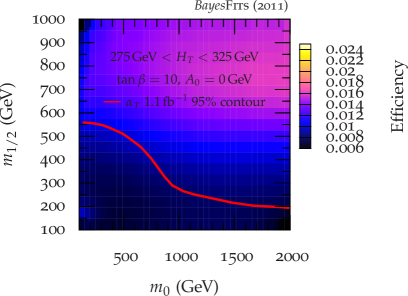
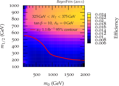
For the selection defined above, we prepared eight efficiency maps, one for each $H_{T}$ bin, two of which are shown as examples in Fig. 1.

$H_{T}$ Bin (GeV)	$275-325$	$325-375$	$375-475$	$475-575$	$575-675$	$675-775$	$775-875$	$>875$
$p_{T}^{\rm leading}$ (GeV)	$73$	$87$	$100$	$100$	$100$	$100$	$100$	$100$
$p_{T}^{\rm second}$ (GeV)	$73$	$87$	$100$	$100$	$100$	$100$	$100$	$100$
$p_{T}^{\rm others}$ (GeV)	$37$	$43$	$50$	$50$	$50$	$50$	$50$	$50$
Observed events
$\alpha_{T}>0.55$	$782$	$321$	$196$	$62$	$21$	$6$	$3$	$1$

Table 2: Definition of the $H_{T}$ bins and the corresponding $p_{T}$ thresholds for the leading, second, and all other remaining jets in the event. Observed events refers to the number of events passing all $\alpha_{T}$ cuts for $1.1/\text{fb}$ of data collected by the CMS CollaborationCMS:2011 .

Experimental selections involving missing transverse energy estimates and selections from an analysis of the distance between a jet and $H_{T}$ were not implemented, because the relevant variables calculated at the generator level are not reliable. Nevertheless, as discussed below, good agreement between efficiency maps obtained in this analysis, and the CMS result shows that such an approximation is justified.

II.3 The likelihood from the CMS $\alpha_{T}$$1.1/\text{fb}$ analysis

The approximate efficiency maps derived in Sec. II.2 for the $\text{CMS}\ \alpha_{T}\ 1.1/\text{fb}$ limit allow us to evaluate a likelihood, so that we can find the regions of the CMSSM’s parameter space in best agreement with the currently strongest LHC limit.

We assume that the experiment can be described by a Poisson distribution; that is, that the events were independent and that the likelihood of observing events was described by a Poisson distribution. We assume that the total number of observed events was the sum of contributions from supersymmetric processes and from SM processes. Following the $\alpha_{T}$ cuts described in Sec. II.2, we consider separately the eight bins of the kinematical variable $H_{T}$ summarized in Table 2.

The number of supersymmetric events that we expected in an $i$-th $H_{T}$ bin, $s_{i}$, is the product of the detector efficiency for that bin (the fraction of events that survive the $\alpha_{T}$ cuts), $\epsilon_{i}$, the integrated luminosity, $\int L=1.1/\text{fb}$, and the total cross section for the production of supersymmetric particles at $\sqrt{s}=7\,\text{TeV}$, $\sigma$,

$$s_{i}=\epsilon_{i}\times\sigma\times\int L.$$ (9)

The likelihood for this case, $\mathcal{L}$, which is the probability of observing a set of $\{o_{i}\}$ events given that we expected $\{s_{i}\}$ supersymmetric events and $\{b_{i}\}$ SM background events, is a product of Poisson distribution for each bin with means $\lambda_{i}=s_{i}+b_{i}$,

$$\mathcal{L}=\prod_{i}\frac{e^{-(s_{i}+b_{i})}\left(s_{i}+b_{i}\right)^{o_{i}}}{o_{i}!}.$$ (10)

We assume that Standard Model backgrounds, $b_{i}$, are precisely known. If their experimental errors were significant, the expression for the likelihood would be multiplied by distributions describing the SM backgroundsLoparco:2011yr and they would be included as nuisance parameters. This is not the case for the $\alpha_{T}$ analysis.

(a)

(b)

Figure 2: The maps of (a) the likelihood and (b) the profile likelihood for our approximation to the $\text{CMS}\ \alpha_{T}\ 1.1/\text{fb}$ analysis on the ($m_{0}$, $m_{1/2}$) plane. The dashed blue lines show the official CMS $95\%$ exclusion contour.

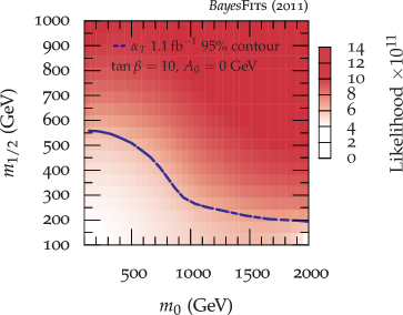
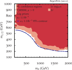
All-hadronic final-state processes are expected to be independent of $\tan\beta$ and $A_{0}$, because these parameters have little influence on the squark and gluino masses, and this has been confirmed by the CMS Collaboration in the $\text{CMS}\ \alpha_{T}\ 1.1/\text{fb}$ analysis, as well as, e.g., in Ref.Allanach:2011ut ; Bechtle:2011dm , and also in this study. For this reason we created efficiency maps using the mentioned earlier fixed-grid scan with fixed values of $\tan\beta=10$ and $A_{0}=0$, as described in Sec. II.2. The cross section was calculated to leading order with PYTHIASjostrand:2000wi . We used this information to produce a likelihood map using Eq. 9 and Eq. 10.

The resulting likelihood map is shown in Fig. 2a. It exhibits the correct behavior; below the official $95$% contour obtained by $\text{CMS}\ \alpha_{T}\ 1.1/\text{fb}$ analysisCMS:2011 , which is also indicated, the likelihood is small. Our approximate $95$% contour was calculated with the help of Eq. 6. It corresponds to the boundary of the $2\sigma$ range of the profile likelihood obtained using Nested Sampling and a log prior, which is shown in Fig. 2b, and is very close to the official CMS contour which is also shown in the Figure. For each CMSSM point for which our scanning algorithm wished to evaluate the likelihood, we interpolated the likelihood from our likelihood map.

III Results

In this section we will present our numerical results. To start with, in Table 1 we show prior ranges and distributions of CMSSM parameters and of SM nuisance parameters, while in Table 3 we list the observables that we will use in our analysis. These come in three sets. First, by “Non-LHC” we collectively denote all relevant constraints from dark matter, $\Omega_{\chi}h^{2}$, precision measurements: $\sin^{2}{\theta}_{\rm eff}$, $M_{W}$, etc, flavour physics: $\mathcal{BR}\left(\bar{B}\rightarrow X_{s}\gamma\right)$, $\mathcal{BR}\left(B_{u}\rightarrow\tau\nu\right)$, $\Delta M_{B_{s}}$, and $\mathcal{BR}\left(B_{s}\rightarrow\mu^{+}\mu^{-}\right)$, the excess in the anomalous magnetic moment of the muon, $\delta(g-2)_{\mu}^{\rm SUSY}$, as well as LEP and Tevatron limits on the Higgs sector and superpartner masses. Second, we will apply currently the best limit published by the CMS Collaboration, which is from its $\alpha_{T}$ analysis of 1.1$/\text{fb}$ of data. Finally, at the end we will also apply an upper limit on the elastic scattering of neutralino dark matter $\sigma_{p}^{\rm SI}$ recently published by XENON100, in order to investigate its additional impact on the CMSSM’s parameters and various observables.

Measurement	Mean	Exp. error	The. error	Likelihood distribution	Reference
$\text{CMS}\ \alpha_{T}\ 1.1/\text{fb}$ analysis
$\alpha_{T}$	See text	See text	$0$	Poisson	CMS:2011
XENON100
$\sigma_{p}^{\rm SI}\left(m_{\chi}\right)$	$<f\left(m_{\chi}\right)$, see text	$0$	$1000\%$	Upper limit: error function	Aprile:2011dd
Non-LHC
$\Omega_{\chi}h^{2}$	$0.1120$	$0.0056$	$10\%$	Gaussian	Komatsu:2010fb
$\sin^{2}{\theta}_{\rm eff}$	$0.231\,16$	$0.000\,13$	$0.000\,15$	Gaussian	Nakamura:2010zzi
$M_{W}$	$80.399$	$0.023$	$0.015$	Gaussian	Nakamura:2010zzi
$\delta(g-2)_{\mu}^{\rm SUSY}$$\times 10^{10}$	$30.5$	$8.6$	$1.0$	Gaussian	Nakamura:2010zzi ; Miller:2007kk
$\mathcal{BR}\left(\bar{B}\rightarrow X_{s}\gamma\right)$$\times 10^{4}$	$3.60$	$0.23$	$0.21$	Gaussian	Nakamura:2010zzi
$\mathcal{BR}\left(B_{u}\rightarrow\tau\nu\right)$$\times 10^{4}$	$1.66$	$0.66$	$0.38$	Gaussian	Asner:2010qj
$\Delta M_{B_{s}}$	$17.77$	$0.12$	$2.40$	Gaussian	Nakamura:2010zzi
$\mathcal{BR}\left(B_{s}\rightarrow\mu^{+}\mu^{-}\right)$	$<1.5\times 10^{-8}$	$0$	$14\%$	Upper limit: error function	Aaij:2011rja
Nuisance
$1/\alpha_{\text{em}}(M_{Z})^{\overline{MS}}$	$127.916$	$0.015$	$0$	Gaussian	Nakamura:2010zzi
$m_{t}^{pole}$	$172.9$	$1.1$	$0$	Gaussian	Nakamura:2010zzi
$m_{b}(m_{b})^{\overline{MS}}$	$4.19$	$0.12$	$0$	Gaussian	Nakamura:2010zzi
$\alpha_{s}(M_{Z})^{\overline{MS}}$	$0.1184$	$0.0006$	$0$	Gaussian	Nakamura:2010zzi
LEP and Tevatron $95$% limits
$m_{h}$	$>114.4$	$0$	$3$	Lower limit: error function	Barate:2003sz
$\zeta_{h}^{2}$	$<f\left(m_{h}\right)$	$0$	$0$	Upper limit – step function	Barate:2003sz
$m_{\chi}$	$>50$	$0$	$5$%	Lower limit: error function	Heister:2003zk (Heister:2001nk ; *Achard:2003ge)
$m_{\chi^{\pm}_{1}}$	$>103.5$ ($92.4$)	$0$	$5$%	Lower limit: error function	lepsusy (Heister:2001nk ; *Achard:2003ge)
$m_{\tilde{e}_{R}}$	$>100$ ($73$)	$0$	$5$%	Lower limit: error function	lepsusy (Heister:2001nk ; *Achard:2003ge)
$m_{\tilde{\mu}_{R}}$	$>95$ ($73$)	$0$	$5$%	Lower limit: error function	lepsusy (Heister:2001nk ; *Achard:2003ge)
$m_{\tilde{\tau}_{1}}$	$>87$ ($73$)	$0$	$5$%	Lower limit: error function	lepsusy (Heister:2001nk ; *Achard:2003ge)
$m_{\tilde{\nu}}$	$>94$ ($43$)	$0$	$5$%	Lower limit: error function	Abdallah:2003xe (Nakamura:2010zzi )
$m_{\tilde{t}_{1}}$	$>95$ ($65$)	$0$	$5$%	Lower limit: error function	lepsusy (Heister:2001nk )
$m_{\tilde{b}_{1}}$	$>95$ ($59$)	$0$	$5$%	Lower limit: error function	lepsusy (Heister:2001nk )
$m_{\tilde{q}}$	$>375$	$0$	$5$%	Lower limit: error function	Abazov:2009zi
${{m_{\tilde{g}}}}$	$>289$	$0$	$5$%	Lower limit: error function	Abazov:2009zi

Table 3: The experimental measurements that constrain the CMSSM’s parameters and the Standard Model’s nuisance parameters. Masses are in GeV. The numbers in parentheses in the list of LEP and Tevatron experimental measurements are weaker experimental bounds, which we use for some sparticle mass hierarchies.

Below we will present the results of our scans as one-dimensional (1D) or two-dimensional (2D) marginalized posterior pdf maps of the CMSSM’s parameters and observables. In evaluating the posterior pdfs, we marginalized over the CMSSM’s other parameters and the SM’s nuisance parameters,

III.1 Impact of the $\alpha_{T}$ limit

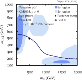
First, in Fig. 3, on the ($m_{0}$, $m_{1/2}$) plane, we show the results of a scan with a likelihood from the non-LHC constraints (left panel) and with the additional impact of imposing the $\alpha_{T}$ $1.1/\text{fb}$ constraint (right panel). Dark (light) blue regions denote the $1\sigma$ ($2\sigma$) posterior pdf regions of the ($m_{0}$, $m_{1/2}$) plane. In Fig. 3a one can see two distinct modes on the ($m_{0}$, $m_{1/2}$) plane. The vertical $1\sigma$ mode is located in in the stau coannihilation/$A$–funnel (SC/AF) region, while the associated $2\sigma$ region is caused by the AF only. On the opposite side of the diagonal of the ($m_{0}$, $m_{1/2}$) plane, the horizontal mode corresponds to overlapping contributions from the light Higgs resonance region (the narrow $1\sigma$ strip) and, above it, the $2\sigma$ focus point (FP)/horizontal branch (HB) region.

As a result, the posterior mean (denoted by a solid black dot) lies between the two modes, but closer to the SC/AF region, where the best-fit point (denoted by an encircled cross) is also located. The blue dashed line denoting the $95\%$ lower limit derived by the $\text{CMS}\ \alpha_{T}\ 1.1/\text{fb}$ analysis is marked, but not applied here.

The existence of the two broad regions is consistent with the findings of previous pre-LHC Bayesian analyzesdeAustri:2006pe ; Roszkowski:2007fd ; Feroz:2008wr ; Trotta:2008bp , although their relative size does depend on the choice of the prior. Physically they both arise as a result of reducing the relic density of the neutralino, which is generally too large in the part of the ($m_{0}$, $m_{1/2}$) plane where $\chi$ is the lightest superpartner. In the SC region the density is reduced by a coannihilation with the lighter stau (and other sleptons), and likewise in the AF region it is reduced by neutralino pair annihilation through the pseudoscalar Higgs $A$–funnel, hence the name. Likewise, the same mechanism is at play in the narrow horizontal light Higgs resonance region. In the FP region, on the other hand, as one moves down along a line roughly perpendicular to the diagonal of the ($m_{0}$, $m_{1/2}$) plane, the value of $\mu^{2}$ drops down from large values (for which the Lightest Supersymmetric Particle (LSP) is very binolike, with too large $\Omega_{\chi}h^{2}$), and eventually becomes negative, implying a failure of radiative electroweak symmetry breaking conditions. Close to this boundary, in a rather narrow strip of the plane, $\mu$ is of order $m_{1/2}$, the LSP develops a sizable Higgsino component, and the relic abundance becomes acceptable.

(a)

(b)

Figure 3: Marginalised posterior pdf on the ($m_{0}$, $m_{1/2}$) plane, LABEL:sub@fig:Comparison_m0m12_lhc-a before and LABEL:sub@fig:Comparison_m0m12_lhc-b after we included a likelihood from the $\text{CMS}\ \alpha_{T}\ 1.1/\text{fb}$ limit.

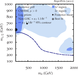
The impact of the $\text{CMS}\ \alpha_{T}\ 1.1/\text{fb}$ limit, which is implemented in our analysis by simulating detector efficiency and evaluating the corresponding likelihood, as described in Sec. II.3, is shown in Fig. 3b. Clearly, the $\alpha_{T}$ limit has cut deep into the ($m_{0}$, $m_{1/2}$) plane’s high posterior probability regions – a nominal fraction of the posterior pdf $1\sigma$ region is outside of the $\alpha_{T}$ 95% confidence interval. The $\alpha_{T}$ limit pushed the credible regions, as well as the best-fit point, to larger values of $m_{1/2}$. Significantly, the two modes on the ($m_{0}$, $m_{1/2}$) plane have remained. The $1\sigma$ SC/AF region has been pushed up nearly vertically, while the $2\sigma$ one of AF only has become inflated and extended to larger values of ($m_{0}$, $m_{1/2}$). Note also that the horizontal light Higgs resonance region has now completely disappeared. On the other hand, the FP/HB region is not excluded by the $\text{CMS}\ \alpha_{T}\ 1.1/\text{fb}$ limit; rather, it is pushed to larger values of $m_{0}$ and, to a lesser extent, $m_{1/2}$.

An analogous comparison of the pre- and post-$\alpha_{T}$ situation in the ($A_{0}$, $\tan\beta$) plane is presented in Fig. 4a and Fig. 4b. There are again two $1\sigma$ modes: one at relatively small values of $\tan\beta\mathrel{\hbox to0.0pt{\lower 4.0pt\hbox{\hskip 1.0pt$\sim$}\hss}\raise 1.0pt\hbox{$<$}}20$ and the other one at much larger values ($\sim 55$), although at $2\sigma$ an entire range of scanned values of $\tan\beta$ is allowed. The first mode corresponds to the $1\sigma$ stau coannihilation region in Fig. 3b; however, in the much larger, $2\sigma$, mostly $A$-funnel region of the ($m_{0}$,$m_{1/2}$) plane much larger values of $\tan\beta\sim 55$ are predominant. On the other hand, in in the focus point region of large $m_{0}$ in Fig. 3b we find $25\mathrel{\hbox to0.0pt{\lower 4.0pt\hbox{\hskip 1.0pt$\sim$}\hss}\raise 1.0pt\hbox{$<$}}\tan\beta\mathrel{\hbox to0.0pt{\lower 4.0pt\hbox{\hskip 1.0pt$\sim$}\hss}\raise 1.0pt\hbox{$<$}}55$.

We can see that the application of the $\alpha_{T}$ constraint narrows down both modes in the posterior pdf on the ($A_{0}$, $\tan\beta$) plane, primarily as a result of pushing up and out the focus point region, with the effect of strongly disfavoring midrange values of $\tan\beta$. On the other hand the CMS limit shows fairly little effect on $A_{0}$, which remains poorly determined.

(a)

(b)

Figure 4: Marginalised posterior pdf on the ($A_{0}$, $\tan\beta$) plane, LABEL:sub@fig:Comparison_a0tanb_lhc-a before and LABEL:sub@fig:Comparison_a0tanb_lhc-b after we included a likelihood from the $\text{CMS}\ \alpha_{T}\ 1.1/\text{fb}$ limit.

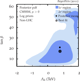
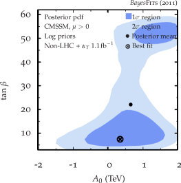
Although our $\alpha_{T}$ likelihood is independent of $\tan\beta$ and $A_{0}$, it is clear from Fig. 4 that $\alpha_{T}$ does impact these parameters. The CMSSM’s parameters are correlated in a nontrivial way; once the $\alpha_{T}$ limit is added to the likelihood it alters the best-fitting values of $m_{0}$ and $m_{1/2}$  and the values of $\tan\beta$ and $A_{0}$ must be adjusted accordingly, so that the predicted values for the CMSSM’s observables maintain agreement with the experimental measurements.

In Fig. 5 we show 1D marginalized posterior pdf plots for the CMSSM’s parameters, constrained by the non-LHC experiments and by the $\alpha_{T}$ limit. We also show the dark (light) blue horizontal bars which indicate the one- (two-) dimensional central credible regions. The high probability modes in the $m_{0}$ distributions at $m_{0}\sim 200\,\text{GeV}$ in Fig. 5a and in the $m_{1/2}$ distribution at $m_{1/2}\sim 700\,\text{GeV}$ in Fig. 5b correspond to the high probability mode in the SC/AF region in Fig. 3b. Fig. 5c shows that the experimental constraints favor positive values of $A_{0}$. The two modes in the $\tan\beta$ distribution in Fig. 5d correspond to the two modes in Fig. 4.

After marginalisation, it is difficult to identify in the $m_{0}$ 1D marginalized posterior pdf the FP/HB mode, which was present in the 2D marginalized posterior pdf in Fig. 3, though it is present as a second smaller mode in the $m_{1/2}$ 1D marginalized posterior pdf in Fig. 5b. This is caused by the contribution of the large $2\sigma$ credible region at both large $m_{1/2}$ and $m_{0}$.

In Fig. 6 we present 1D plots of marginalized posterior pdf for notable particle masses, when we scanned the CMSSM with a likelihood from $\alpha_{T}$ and from the non-LHC experiments. These distributions are typically bimodal; one mode is from the mode in the SC/AF region and one mode is from the mode in the FP/HB region on the ($m_{0}$, $m_{1/2}$) plane in Fig. 3.

(a)

(b)

(c)

(d)

Figure 5: One-dimensional marginalized posterior pdf for the CMSSM’s parameters constrained by the $\text{CMS}\ \alpha_{T}\ 1.1/\text{fb}$ analysis and by the non-LHC experiments. The dark (light) blue horizontal bars span the one- (two-)dimensional central credible regions.

(a)

(b)

(c)

(d)

Figure 6: The mass of the lightest LABEL:sub@fig:4masses-a squark, LABEL:sub@fig:4masses-b gluino, LABEL:sub@fig:4masses-c neutralino, and LABEL:sub@fig:4masses-d Higgs-boson in the CMSSM constrained by $\alpha_{T}$ and by the non-LHC experiments. The horizontal bars have been defined in Fig. 5.

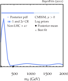
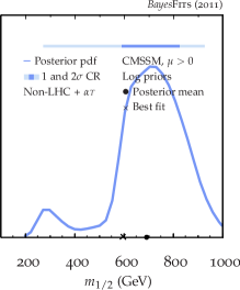
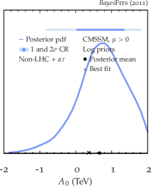
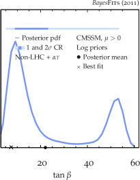
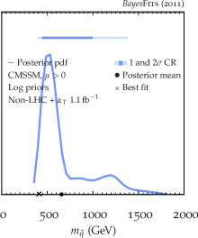
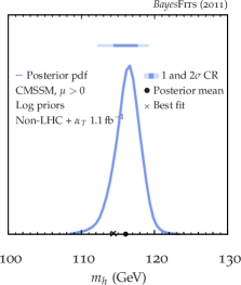
Fig. 6a shows that the posterior favors a moderately heavy lightest squark (the lighter stop) with $m_{\tilde{q}}\sim 500\,\text{GeV}$, corresponding to the mode in the SC/AF region with small $m_{0}\sim 100\,\text{GeV}$. There is a second, much smaller, mode in the posterior at $m_{\tilde{q}}\sim 1250\,\text{GeV}$, corresponding to the mode in the FP/HB region with large $m_{0}\sim 2000\,\text{GeV}$. On the other hand, the squarks of the first two generations can be much heavier, up to $\sim 2.7\,\text{TeV}$ at $1\sigma$.

Heavy gluinos, much heavier than lightest squarks, are favored with ${m_{\tilde{g}}}\sim 1500\,\text{GeV}$, as illustrated in Fig. 6b. This dominant range corresponds to the mode in the SC/AF region with large $m_{1/2}\sim 700\,\text{GeV}$. Lighter gluinos with ${m_{\tilde{g}}}\lesssim 1000\,\text{GeV}$ are not, however, excluded, by the credible region. This is a result of the mode in the FP/HB region.

Fig. 6c shows that the posterior pdf favors a lightest neutralino mass of $m_{\chi}\sim 300\,\text{GeV}$. This corresponds to a binolike neutralino, with $m_{\chi}\sim 0.4m_{1/2}$.

Lastly, Fig. 6d shows the 1D posterior pdf for the mass of the lightest Higgs in the CMSSM, in agreement with pre-LHC resultsdeAustri:2006pe ; Allanach:2007qk ; Trotta:2008bp ; Buchmueller:2010ai .

The lightest Higgs boson in the CMSSM is to a very good approximation SM like and the LEP limit ($114.4\,\text{GeV}$) applies. Note, however, that predicted Higgs masses below the LEP limit are permitted, because our likelihood function includes a $3\,\text{GeV}$ theoretical error in the predicted Higgs mass. On the other side, the 1D posterior pdf is rather narrow, with the $95$% credible region in the range from $112.2\,\text{GeV}$ to $119.2\,\text{GeV}$ and the best-fit value of $114.4\,\text{GeV}$.

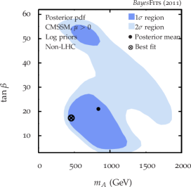
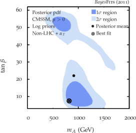
Being SM like, the lightest Higgs boson may well be the only Higgs state of the CMSSM accessible in Run I. The other Higgses are typically nearly mass degenerate, and much heavier than the lightest Higgs. This is illustrated in Fig. 7, where we present a 2D posterior pdf map on the ($m_{A}$, $\tan\beta$) plane in two cases: pre-$\alpha_{T}$ (left panel) and post-$\alpha_{T}$ (right panel). Fig. 7 shows that the $\alpha_{T}$ limit favors a heavier CP-odd neutral Higgs, because it favors higher values of $m_{0}$. Intermediate values of $\tan\beta\sim 30$, however, are disfavored by $\alpha_{T}$, and, consequently, very heavy CP-odd neutral Higgs with $m_{A}\gtrsim 1500\,\text{GeV}$ become disfavored.

(a)

(b)

Figure 7: Marginalised posterior pdf on the ($m_{A}$, $\tan\beta$) plane, LABEL:sub@fig:Comparison_mAtanbeta-a before and LABEL:sub@fig:Comparison_mAtanbeta-b after we included a likelihood from the $\text{CMS}\ \alpha_{T}\ 1.1/\text{fb}$ limit.

III.2 Impact of the XENON100 limit

The XENON100 Collaboration has recently published a new $90$% C.L. exclusion limit on the ($m_{\chi}$, $\sigma_{p}^{\rm SI}$) plane which significantly improves their previous preliminary limitAprile:2011hi . In this section we examine the impact of this new limit on the CMSSM’s parameters and observables.

A proper implementation of the XENON100 exclusion limit in our likelihood function is somewhat tricky. The $90$% exclusion contour alone is insufficient to reconstruct the likelihood function. On top of it, there are significant errors, which originate from poorly known inputs which are needed in evaluating a limit on $\sigma_{p}^{\rm SI}$ from experimental data. First, one assumes a “default” value for the local density of $0.3\,\text{GeV}/c^{2}$, but errors in astrophysical parameters which are required to determine the local halo and its velocity distribution can result in errors in $\sigma_{p}^{\rm SI}$ of order $2$Pato:2010zk , although a much better determination has been claimedCatena:2009mf . More significantly, the fractional error in evaluating $\sigma_{p}^{\rm SI}$ coming from uncertainties in inputs to hadronic matrix elements can be of order $5$, as discussed in detail inBuchmueller:2011ki . The main uncertainty is due to a poor knowledge of the $\pi$-nucleon $\sigma$ term, $\Sigma_{\pi N}$, which determines the strange quark component of the nucleon.

Given these large uncertainties, we neglect the experimental error in the XENON100 $90$% exclusion contour and approximate it in the likelihood with a step function, $\mathcal{L}(\sigma_{p}^{\rm SI},m_{\chi})=0(1)$ for $\sigma_{p}^{\rm SI}>(\leq)\sigma^{\rm SI}_{p,\,90\%}(m_{\chi})$, where $\sigma^{\rm SI}_{p,\,90\%}(m_{\chi})$ is the DM mass dependent XENON100 90% limit. To incorporate the above errors in evaluating $\sigma_{p}^{\rm SI}$ in a conservative way, we convolute the step function with a Gaussian with $\mu=\sigma_{p}^{\rm SI}$ and $\sigma=10\times\sigma_{p}^{\rm SI}$, resulting in a Gaussian error function. This will cause a rather large smearing out of the XENON100 limit.

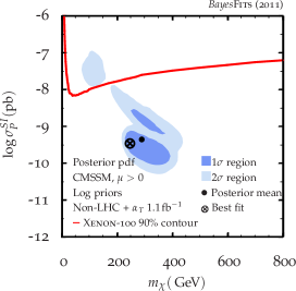
This can be seen in Fig. 8 where we present the impact of the XENON100 90% C.L. limit (denoted with solid red curve) on probability maps of the ($m_{\chi}$, $\sigma_{p}^{\rm SI}$) plane for our scans. In Fig. 8a the XENON100 limit is not added to the likelihood, while in Fig. 8b it is applied. By comparing both panels we can see that, once LHC limits have been applied (left panel), the $1\sigma$ posterior region on the ($m_{\chi}$, $\sigma_{p}^{\rm SI}$) plane is only weakly affected by the additional XENON100 limit (right panel).

Some interesting effects can nevertheless be noticed. First, a small $2\sigma$ region above the XENON100 exclusion curve has shrunk somewhat, especially on the side of larger $\sigma_{p}^{\rm SI}$, but, because of the large theoretical error assumed in this analysis, it remains allowed. Second, the large smearing affects the favored regions of $\sigma_{p}^{\rm SI}$ also below the experimental curve. Note that, before the XENON100 is applied (Fig. 8a) there are actually two $1\sigma$ regions close to each other. The lower one comes entirely from the stau-coannhilation region of small $m_{0}$ and large $m_{1/2}$. The other one, just above it (along with a broader $2\sigma$ region, both decreasing with $m_{\chi}$), corresponds to the broad $2\sigma$ AF region in the ($m_{0}$, $m_{1/2}$) plane. Once the XENON100 limit is added to the likelihood (Fig. 8b), the largest values of $\sigma_{p}^{\rm SI}$, just below the experimental curve, become excluded and the statistical significance of the whole AF region becomes reduced to the $2\sigma$ level. On the other hand, the lower $1\sigma$ region remains nearly intact.

Clearly, recent LHC limits have had the effect of pushing down the most favored ranges of $\sigma_{p}^{\rm SI}$, for the most part below $\sim 10^{-9}\,\text{pb}$, while pre-LHC data favored largest $1\sigma$ posterior ranges of $\sigma_{p}^{\rm SI}$ at least an order of magnitude higher; compare, e.g.,Roszkowski:2007fd ; Trotta:2008bp . This implies much poorer prospects for XENON100, with expected reach of $\sim 10^{-9}\,\text{pb}$ to explore the SI cross sections currently favored by the CMSSM.

It is also clear that, in light of the impact of LHC limits, one-ton detectors with planned sensitivity reach of $\sim 10^{-10}\,\text{pb}$ will now be needed to explore the most probable ranges of the ($m_{\chi}$, $\sigma_{p}^{\rm SI}$) plane in the CMSSM. We also note that the most probable range of dark matter particle mass, $250\,\text{GeV}\mathrel{\hbox to0.0pt{\lower 4.0pt\hbox{\hskip 1.0pt$\sim$}\hss}\raise 1.0pt\hbox{$<$}}m_{\chi}\mathrel{\hbox to0.0pt{\lower 4.0pt\hbox{\hskip 1.0pt$\sim$}\hss}\raise 1.0pt\hbox{$<$}}343\,\text{GeV}$ (at $1\sigma$) is somewhat above the range of the highest sensitivity of most detectors. Finally, in Table 4, we show the combined impact of the $\alpha_{T}$ and xenon limits on the posterior ranges of several particle masses already constrained by other (Non-LHC) data. The $1\sigma$ and $2\sigma$ posterior ranges were calculated with Eq. 5.

(a)

(b)

Figure 8: Marginalised posterior pdf on the ($\sigma_{p}^{\rm SI}$, $m_{\chi}$) plane, LABEL:sub@fig:Comparison_sigsipmchi-a before and LABEL:sub@fig:Comparison_sigsipmchi-b after we included a likelihood for the XENON100 limit.

(a)

(b)

Figure 9: Marginalised posterior pdf with the log prior the CMSSM’s parameters constrained by non-LHC experiments, the $\text{CMS}\ \alpha_{T}\ 1.1/\text{fb}$ limit and the XENON100 limit. The panels should be compared with the corresponding panels in Fig. 3 and Fig. 4.

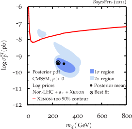
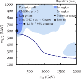
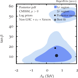
Finally, in Fig. 9, we show the impact of the XENON100 limit on the shapes of the 2D marginalized posterior pdf maps for the CMSSM parameters. The results shown here correspond to a scan with a likelihood from the non-LHC constraints, from the $\text{CMS}\ \alpha_{T}\ 1.1/\text{fb}$ analysis and from XENON100. The panels should be compared with the corresponding panels in Fig. 3 and Fig. 4.

The discussion of Fig. 8 above helps in understanding new effects in Fig. 9. First, it is clear that, the configurations of the CMSSM parameters are already constrained by current LHC limits to give $\sigma_{p}^{\rm SI}$ for the most part below the XENON100 limit. Unsurprisingly, adding it to the likelihood has a relatively weak additional impact on the CMSSM’s parameters. The $1\sigma$ posterior region in the high probability SC region on the ($m_{0}$, $m_{1/2}$) plane in Fig. 9a remains unaffected because the corresponding values of $\sigma_{p}^{\rm SI}$ are the lowest. The change in the best-fit point is also probably not statistically significant. However, note that the broader $2\sigma$ region of AF has shrunk somewhat on the side of large $m_{0}$, especially in the direction of the HB/FP region. This is because in that direction the Higgsino component of the DM neutralino increases, causing in turn $\sigma_{p}^{\rm SI}$ to increase and become at some point constrained by the XENON100 limit, especially for large $\tan\beta$.

Moving farther toward the lower-right corner, we can see that the XENON100 result disfavors also the HB/FP region – the $1\sigma$ credible region in the ($m_{0}$, $m_{1/2}$) plane in Fig. 3a has now become only a $2\sigma$ region. This is not surprising since predicted values of $\sigma_{p}^{\rm SI}$ in that regions are among the largest predicted in the CMSSM, again because of the increased Higgsino component of the neutralino. We stress, however, that the HB/FP region is not excluded by the XENON100 limit; rather, it is inside the $2\sigma$ credible region. This follows from our conservative estimation of the error in the $\sigma_{p}^{\rm SI}$ calculation. (We weakened the XENON100 limit by smearing it with a Gaussian describing the theoretical error in the $\sigma_{p}^{\rm SI}$ calculation.) We have checked that, if we assumed the theoretical error in $\sigma_{p}^{\rm SI}$ to be $0.1\times\sigma_{p}^{\rm SI}$, the XENON100 limit would exclude the focus point region at $2\sigma$. Finally we note that the favored regions on the ($A_{0}$, $\tan\beta$) plane in Fig. 9b are not strongly affected by XENON100, though the two modes on the ($A_{0}$, $\tan\beta$) plane are no longer connected.

Mass (GeV)	$68$%	$95$%	$68$%	$95$%
	Non-LHC		Non-LHC + $\text{CMS}\ \alpha_{T}\ 1.1/\text{fb}$ limit + XENON100
$m_{h}$	$(112.3,116.5)$	$(110.1,118.4)$	$(114.4,117.8)$	$(112.2,119.4)$
$m_{\chi}$	$(56,291)$	$(53,356)$	$(250,343)$	$(128,390)$
$m_{{\chi}^{\pm}_{1}}$	$(110,554)$	$(104,676)$	$(475,651)$	$(181,738)$
$m_{\tilde{q}}$	$(326,808)$	$(254,1172)$	$(434,761)$	$(398,1302)$
${m_{\tilde{g}}}$	$(403,1576)$	$(384,1885)$	$(1380,1825)$	$(879,2043)$

Table 4: Posterior $1\sigma$ and $2\sigma$ regions for several particle masses, when constrained by pre- (two left columns) and post-$\text{CMS}\ \alpha_{T}\ 1.1/\text{fb}$ data, calculated with Eq. 5.

III.3 Prior dependence and the best-fit point

We will now comment on the prior dependence of the results presented here, and will also come back to the discussion of the best-fit point.

As is well known, some of the most challenging aspects of Bayesian statistics are the necessity to choose a prior and the sensitivity of the posterior to that choice. The prior dependence of the posterior is a measure of the lack of the constraining power of the likelihood function. If the information from data included in the likelihood is sufficient to select ranges of model’s parameters giving good fit to the constraints (high posterior probability regions), then the sensitivity of such ranges to the choice of priors should be weak, or even marginal. In such cases the likelihood has the ability to overpower noninformative priors, such as log priors and linear (flat) priors, and the resulting posterior has little prior dependence. If, however, the posterior is dependent on the choice of prior, the likelihood ought to be regarded as too weak to support robust conclusions about the model.

In several pre-LHC studies prior dependence of the CMSSM was found to be substantial (see, e.g.,Roszkowski:2007fd ; Trotta:2008bp ), and the situation in less constrained models was found to be even less satisfactoryRoszkowski:2009sm . This was merely a reflection of poor constraining power of the data available at that time. It was also concluded that the choice of the prior that is linear in the log of the masses is more motivated by both physical and statistical reasonsRoszkowski:2007fd ; Trotta:2008bp . From the physical point of view, log priors explore in much greater detail the low-mass region, where one typically needs less fine tuning in order to achieve radiative electroweak symmetry breaking. From the statistical point of view, log priors give the same a priori weight to all orders of magnitude in the masses, and thus appear to be less biased to giving larger statistical a priori weights to the large mass region, which under a flat prior has a much larger volume in parameter space.

(a)

(b)

Figure 10: Marginalised posterior pdf with the linear (flat) prior the CMSSM’s parameters constrained by non-LHC experiments, the $\text{CMS}\ \alpha_{T}\ 1.1/\text{fb}$ limit and the XENON100 limit. The Figure should be compared with Fig. 9.

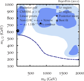
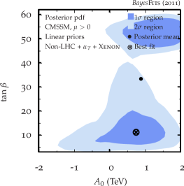
Motivated by the above arguments, in this study we have chosen log priors for the CMSSM’s mass parameters, and our posterior distributions are, of course, dependent on the choice. As a way of examining the degree of the dependence, we identically repeated our scan of the CMSSM with a likelihood from the non-LHC experiments and from $\alpha_{T}$, except that this time we chose linear priors for all the CMSSM’s parameters. The resulting posterior distributions, which are shown in Fig. 10, are actually broadly similar to the distributions that resulted from log priors. With linear priors, we found three $1\sigma$ modes in the marginalized posterior pdf on the ($m_{0}$, $m_{1/2}$) plane, rather than two as in Fig. 3b. The third mode is present in Fig. 10 both large $m_{1/2}$ and $m_{0}$, and probably results from the mentioned above volume effect on the marginalized posterior. For the same reason the $2\sigma$ region at large masses also becomes enhanced and the FP/HB mode again becomes strengthened. We interpret this as a reflection of the fact that, despite new strong limits from the LHC, the constraining power of experimental data remains insufficient to eliminate prior dependence of the CMSSM. On the other hand, the effect of assuming the linear prior for $m_{1/2}$ and $m_{0}$on the parameters $\tan\beta$ and $A_{0}$ appears to be relatively weaker, as expected, since for the latter the prior has been assumed to be the same (linear) in both cases.

Constraints	$m_{0}$	$m_{1/2}$	$A_{0}$	$\tan\beta$	$\chi^{2}$	d.o.f.	$p$-value
Non-LHC	$122$ $(116,1391)$	$343$ $(142,702)$	$806$ $(236,1514)$	$17$ $(13,22)$	$16.53$	$16$	$42\%$
Non-LHC + $\alpha_{T}$ + XENON100	$122$ $(127,741)$	$600$ $(608,820)$	$677$ $(82,1283)$	$11$ $(9,16)$	$22.21$	see text	see text

Table 5: Best-fit points and $68\%$ central credible regions for the CMSSM’s parameters, calculated with Eq. 5, when constrained by different sets of experimental data. Masses are in  GeV. The best-fit values of $m_{0}$ are close to the lower edge of our prior range for $m_{0}$, which is $100\,\text{GeV}$; therefore, our central credible regions exclude the best-fit values of $m_{0}$.

Constraint	$\Omega_{\chi}h^{2}$	$m_{h}$	$\bar{B}\rightarrow X_{s}\gamma$	$\sin^{2}{\theta}_{\rm eff}$	$M_{W}$	$\delta(g-2)_{\mu}^{\rm SUSY}$	$B_{u}\rightarrow\tau\nu$	$\Delta M_{B_{s}}$	$\alpha_{T}$	Total
$\chi^{2}$	$0.01$	$1.32$	$1.98$	$4.16$	$1.49$	$9.76$	$0.03$	$0.25$	$3.42$	$22.21$

Table 6: Breakdown of the main contributions to $\chi^{2}$ for our best-fit point from a scan with a likelihood from non-LHC experiments and the $\alpha_{T}$ and XENON100 limits. Note that all likelihoods are normalized to unity, including one for each $H_{T}$ bin.

On the other hand, the location of the best-fit point should, by definition, be entirely determined by the likelihood function, and therefore independent of the prior. However, because in practice it is found numerically with a Monte Carlo method, it is a random variable with an error and with a weak dependence on the scanning algorithm, rather than an exact solution. This is clear when one remembers that by choosing, for example, the log prior for the CMSSM’s mass parameters, one in practice also chooses a log metric for these parameters. As a result, the scanning algorithm inevitably explores the low-mass region of the CMSSM’s ($m_{0}$, $m_{1/2}$) plane in greater detail than the high-mass region. This metric dependence can be overcome, or at least reduced, by tightening the algorithm’s stopping conditions, so that it runs until it has explored the whole parameter space in sufficient detail. We also emphasise once again that, in Bayesian statistics the best-fit point has no significance.

In Table 5 we present best-fit points from two scans of the CMSSM: one with non-LHC constraints only and one with $\alpha_{T}$ and XENON100 constraints added to the likelihood. (We quote our best-fit points rounded to the nearest whole  GeV or unit of $\tan\beta$.) In both cases the best-fit point is located in the SC/AF region of the CMSSM’s parameter space. Our best-fit point for the non-LHC-only case is in good agreement with best-fit points reported previously in Ref.deAustri:2006pe ; Allanach:2007qk ; Trotta:2008bp ; Buchmueller:2010ai , which is encouraging. Our $p$-value of $42\%$ is also reasonably close to MasterCode’s latest result for the CMSSM of $37\%$ for this caseRef.Buchmueller:2011sw .

On the other hand, after including the $\alpha_{T}$ and XENON100 constraints in the likelihood, our best-fit point shifts up almost vertically to a larger value of $m_{1/2}\simeq 600\,\text{GeV}$, while the one in Ref.Buchmueller:2011sw moves much more radically, to much larger values of both mass parameters ($m_{0}=450\,\text{GeV}$ and $m_{1/2}=780\,\text{GeV}$), and also giving much larger $\tan\beta=41$, although with large standard deviations reported for all the parameters.

We investigated which constraints included in the likelihood played the most important role in determining the shape of the posterior, and also the location of the best-fit point. In Table 6 we show a breakdown of the main contributions to the $\chi^{2}$ for the best-fit point corresponding to including the $\alpha_{T}$ and XENON100 constraints in the likelihood. (Note that the $\alpha_{T}$ likelihood is itself a product of eight likelihoods, and therefore contributes 8 degrees of freedom, and inevitably has a relatively poor $\chi^{2}$.) It is clear that the constraint from $\delta(g-2)_{\mu}^{\rm SUSY}$ plays the biggest role in increasing the $\chi^{2}$ for the best-fit point.

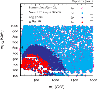
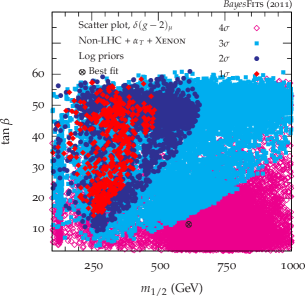
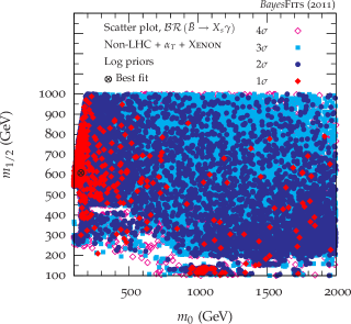
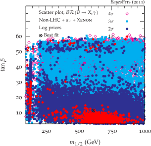
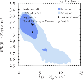
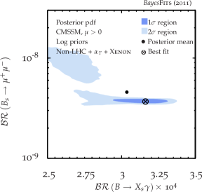
The upper panels of Fig. 11 show that the $\delta(g-2)_{\mu}^{\rm SUSY}$ constraint requires that increases in $m_{1/2}$ induced by the $\alpha_{T}$ limit are compensated by increases in $m_{0}$ [Fig. 11a], and also in $\tan\beta$ [Fig. 11b]. Our best-fit point is, however, being pulled in a different direction mostly by $\mathcal{BR}\left(\bar{B}\rightarrow X_{s}\gamma\right)$. The lower panels of Fig. 11 show that increasing $m_{1/2}$ by improving LHC mass limits, does not require one to increase $m_{0}$ [Fig. 11c] and small $\tan\beta$ is sufficient [Fig. 11d], in order to maintain a good fit to $\mathcal{BR}\left(\bar{B}\rightarrow X_{s}\gamma\right)$. There is a clear tension between on the one hand $\delta(g-2)_{\mu}^{\rm SUSY}$, which favors lighter mass spectra in order to generate large enough SUSY contribution to the variable, and, on the other hand, $\mathcal{BR}\left(\bar{B}\rightarrow X_{s}\gamma\right)$ and other constraints which prefer a SUSY contribution to be all but suppressed. The tension between the two observables is exacerbated by adding the constraint from $\alpha_{T}$, because it pushes $m_{1/2}$ into a region of the ($m_{0}$, $m_{1/2}$) plane in which it is more difficult to satisfy both constraints simultaneously. It appears that, at the end $\delta(g-2)_{\mu}^{\rm SUSY}$ is outweighed by the other constraints, most notably $\mathcal{BR}\left(\bar{B}\rightarrow X_{s}\gamma\right)$. As a result, we find that the best-fit point remains at small $m_{0}$ and $\tan\beta$, and $\delta(g-2)_{\mu}^{\rm SUSY}$ is forsaken. Consequently, the best-fit points have a large $\chi^{2}$ from $\delta(g-2)_{\mu}^{\rm SUSY}$but not from $\mathcal{BR}\left(\bar{B}\rightarrow X_{s}\gamma\right)$; compare Table 6.

To investigate its effect, we repeated our analysis without the $\delta(g-2)_{\mu}^{\rm SUSY}$ experimental constraint. With a likelihood from non-LHC experiments, except for $\delta(g-2)_{\mu}^{\rm SUSY}$, and from $\alpha_{T}$, the credible regions on the ($m_{0}$,$m_{1/2}$) plane are similar to those in Fig. 3b, though the central region of the plane is disfavored. The best-fit point’s value of $m_{1/2}$ is significantly larger than that in Fig. 3b. This suggests that, while it favors smaller values of the SUSY mass parameters, $\delta(g-2)_{\mu}^{\rm SUSY}$ does not play the dominant role in determining the credible regions.

This is further illustrated in of Fig. 12a, where we show the interplay between combinations of constraints from $\mathcal{BR}\left(\bar{B}\rightarrow X_{s}\gamma\right)$, $\mathcal{BR}\left(B_{s}\rightarrow\mu^{+}\mu^{-}\right)$, $\delta(g-2)_{\mu}^{\rm SUSY}$ and $\Omega_{\chi}h^{2}$ in 2D marginalized posteriors. We can also see that the resulting range of $\mathcal{BR}\left(B_{s}\rightarrow\mu^{+}\mu^{-}\right)$ is very close to its SM value and that $\Omega_{\chi}h^{2}$ plays a rather neutral role in determining both the posterior and the best-fit point. This is because one can relatively easily adjust $A_{0}$ to produce the correct value of $\Omega_{\chi}h^{2}$, without much affecting the other major constraints.

(a)

(b)

(c)

(d)

Figure 11: Scatter plots of points from a scan with a likelihood from the $\alpha_{T}$ and XENON100 limits and from non-LHC experiments, colored by the values of $\delta(g-2)_{\mu}^{\rm SUSY}$ (top row) and $\mathcal{BR}\left(\bar{B}\rightarrow X_{s}\gamma\right)$ (bottom row). The colors show the discrepancy between the CMSSM’s predicted value and the central experimental value, measured in experimental errors.

(a) t

(b) t

(c) t

(d) t

Figure 12: Marginalised posterior pdf for combinations of the experimental observables $\mathcal{BR}\left(\bar{B}\rightarrow X_{s}\gamma\right)$, $\delta(g-2)_{\mu}^{\rm SUSY}$, $\mathcal{BR}\left(B_{s}\rightarrow\mu^{+}\mu^{-}\right)$ and $\Omega h^{2}$, from a scan with a likelihood from $\alpha_{T}$, XENON100 and non-LHC experiments.

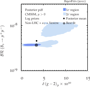
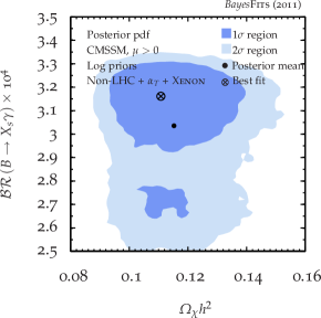
Another note is in order about $\chi^{2}$ and the $p$-value. As can be seen from Table 5, applying only non-LHC constraints, we find $\chi^{2}=16.53$ and the $p$-value of $42\%$. Adding new constraints from the $\alpha_{T}$ and XENON100 likelihood inevitably increases the value of $\chi^{2}$, but a shift in the $p$-value depends on our assumptions about the additional degrees of freedom. In the CMS analysisCMS:2011 the observed events in each bin are treated as independent of the other bins, and described by a Poisson distribution. This is why in our treatment of the $\alpha_{T}$ limit we evaluated likelihood in each of the eight energy bins independently, treating them as contributing as many new degrees of freedom. In this case the $p$-value in fact increases to $61\%$. On the other hand, one could reasonably expect that signal events in different bins would be correlated, in which case the $\alpha_{T}$ constraint could be treated as effectively contributing only one extra degree of freedom. In this case the resulting $p$-value would be 22.3%. This illustrates the difficulty in correctly estimating the number of degrees of freedom and the $p$-value. We also note that in a recent analysis of the MasterCodeBuchmueller:2011sw the $p$-value diminished from $37\%$ to $15\%$ when the LHC and XENON100 constraints were included. Note, however, that in that analysis Gaussian distributions were assumed, unlike here. Also, their way of including LHC limits from jets+$/E_{T}$in the likelihood contributed only 1 additional degree of freedom and also forward-backward scattering variables $A_{\text{fb}}$ were included in their likelihood, which suppressed their $p$-values further. All this makes it difficult to compare the resulting values of $\chi^{2}$ and $p$-value.

In addition to a different location of the best-fit point and the $p$-value, the confidence intervals on the ($m_{0}$, $m_{1/2}$) plane that are found in Ref.Buchmueller:2011sw are much larger than our confidence intervals and span the central region. On the other hand, they do not include the focus point region. In contrast, we find regions of the largest posterior not only in the SC/AF region but also in the focus point region, both in the pre-LHC case, in agreement with previous studies using the SuperBayeS codeTrotta:2008bp , and also after including the $\alpha_{T}$ and XENON100 limits. A physical reason for its existence has been given earlier.

The apparent discrepancy between some of the results reported here and those in a recent $\chi^{2}$ analysis by the MasterCode groupBuchmueller:2011ki is probably caused by a combination of several factors. Some have already been mentioned above. Most likely, the different ways of implementing LHC limits play an important role. We also note that the implementation of $\mathcal{BR}\left(\bar{B}\rightarrow X_{s}\gamma\right)$ in the version of SuperBayeS that we have used for this analysis differs from that of the MasterCode group whose experimental constraint is the ratio of the measured branching ratio to its Standard Model prediction. In contrast, in SuperBayeS the constraint from $\mathcal{BR}\left(\bar{B}\rightarrow X_{s}\gamma\right)$ is simply applied to the measured branching ratio. On the other hand, the choice of different statistics (Bayesian vs $\chi^{2}$) is probably of secondary importance since our results for the best-fit point agree reasonably well in the non-LHC case with several other analyzes, both Bayesian and $\chi^{2}$,Trotta:2008bp ; Allanach:2011ut ; Bechtle:2011it ; Buchmueller:2011aa . We also note that the large $1\sigma$ errors reported on the CMSSM parameters for the best-fit point in Buchmueller:2011ki indicate to us that probably small differences in the likelihood function may lead to large shifts in the location of the best-fit point, in addition to numerical issues related to using different scanning algorithms. This may imply that the high probability regions of the CMSSM parameter space after including current LHC constraints are quite “unstable,” or can fairly easily shift within a rather wide plateau, in the sense that “secondary” issues such as the precise implementation of some of the main constraints, or a treatment of LHC limits may lead to major differences, and seemingly contradictory results.

IV Summary

We have performed an updated Bayesian analysis of the CMSSM. In addition to updating experimental inputs in indirect modes of constraining SUSY [most notably $\mathcal{BR}\left(B_{s}\rightarrow\mu^{+}\mu^{-}\right)$], we included much improved limits from the $\text{CMS}\ \alpha_{T}\ 1.1/\text{fb}$ analysis, which currently gives the strongest bounds on the CMSSM mass parameters, and from the XENON100 experiment. We simulated the $\text{CMS}\ \alpha_{T}\ 1.1/\text{fb}$ analysis in an approximate but methodologically correct way by estimating the efficiency for the $\alpha_{T}$ method and constructing a likelihood function. We validated our method against the official CMS $95\%$ contour. For the XENON100 limit we constructed a conservative, approximate likelihood function by taking into account large uncertainties related to the inputs to hadronic matrix elements and the local density of dark matter.

We incorporated these likelihoods into a global Bayesian fit of the CMSSM and identified marginalized posterior maps of the CMSSM’s parameter space. These credible regions were compared with credible regions before the new experiments to illustrate the effects of the new constraints. The $\alpha_{T}$ limit has taken a deep bite into regions of the CMSSM’s parameter space that were previously favored, and has pushed the best-fit point to significantly higher values of $m_{1/2}$. Including XENON100 in the likelihood had a weak additional effect. We find that, although the focus point region is disfavored by the new constraints, it is still not excluded.

Despite the disappointing null results of SUSY searches at the LHC so far, which have pushed the allowed ranges of CMSSM mass parameters, especially $m_{1/2}$, up to much larger values, we note that the best-fit point, both before and after including the $\text{CMS}\ \alpha_{T}\ 1.1/\text{fb}$ limit, is found close to the bottom of the marginalized $1\sigma$ posterior ranges of both $m_{0}$ and $m_{1/2}$. Despite the uncertainties in determining its location discussed above, this is certainly encouraging for prospects of finding a signal of SUSY in a much larger dataset already collected by both ATLAS and CMS. On the other hand, we note that the preference for the low-mass spectrum in the CMSSM and similar unified models is driven primarily by a single constraint from the $\delta(g-2)_{\mu}^{\rm SUSY}$ anomaly, satisfying what has already been in some tension with $\mathcal{BR}\left(\bar{B}\rightarrow X_{s}\gamma\right)$, and is now becoming increasingly harder also with improving LHC limits.