aainstitutetext: Department of Astronomy and Theoretical Physics, Lund University,
Sölvegatan 14A, SE 223-62 Lund, Sweden

Constraining General Two Higgs Doublet Models by the Evolution of Yukawa Couplings

Johan Bijnens a    Jie Lu a    and Johan Rathsman Johan.Bijnens@thep.lu.se Lu.Jie@thep.lu.se Johan.Rathsman@thep.lu.se
Abstract

We study how general two Higgs doublet models can be constrained by considering their properties under renormalization group evolution of the Yukawa couplings. We take into account both the appearance of a Landau pole as well as off-diagonal Yukawa couplings leading to flavour changing neutral currents in violation with experimental constraints at the electroweak scale. We find that the latter condition can be used to limit the amount of Z2subscript𝑍2Z_{2} symmetry breaking allowed in a given model.

Keywords:
Beyond Standard Model, Higgs Physics
arxiv: 1111.5760

1 Introduction

The Standard Model (SM) has been compared to experiments with great success in the past decades and finding the Higgs boson is the only missing piece. However, there are still a few internal problems. The prime example is the so called hierarchy problem: why is the electroweak (EW) scale much smaller than the Plank scale? Thus, the SM cannot be seen as a fundamental theory of particle physics, but only as an effective description which will break down at higher energies, at least at the Planck scale where gravity becomes of the same magnitude as the gauge forces. The mission of the Large Hadron Collider at CERN is therefore not only to look for the SM Higgs boson but also for physics Beyond the Standard Model (BSM).

The general two Higgs Doublet Model (2HDM) was one of the earliest BSM models, proposed by T.D. Lee Lee:1973iz already in 1973 as a model with spontaneous CP-violation. The 2HDM itself cannot give any solution to the problems of the SM, such as the hierarchy problem. On the contrary, it introduces more problems such as tree level flavour-changing-neutral-currents (FCNC) which are absent in the SM. However, a 2HDM is part of many other BSM models, especially supersymmetric ones, which require an even number of Higgs doublets. Therefore it is useful and interesting to study the 2HDM itself, since it can be thought of as an effective description of more general models at the TeV scale. One such example is the Minimal SuperSymmetric Model (MSSM) in the case of heavy superpartners such that the Higgs bosons only decays to SM particles.

The problem of tree level FCNC can be evaded by introducing an appropriate Z2subscript𝑍2Z_{2} symmetry that ensures that each fermion type only couples to one of the Higgs doublets, which is sufficient in order to avoid tree-level FCNC as shown by Glashow and Weinberg Glashow:1976nt . This is precisely what happens in the MSSM whose Higgs sector at tree-level is a so called type II 2HDM, meaning that one of the Higgs doublets couples only to down-type fermions and the other only to up-type ones. By enforcing a Z2subscript𝑍2Z_{2}-symmetry one also ensures the absence of tree-level FCNC under renormalization group evolution of the model to other energy scales.

Recently another way of avoiding the tree-level FCNC, by having the Yukawa couplings to the two Higgs doublets proportional to each other, has been proposed Pich:2009sp . This works fine at a given energy scale but if one evolves the model to another scale then the tree-level FCNC are reintroduced because the Yukawa couplings in this model do not respect any Z2subscript𝑍2Z_{2} symmetry as shown by Ferreira et al Ferreira:2010xe . There has also been some discussion of the experimental constraints on this model under renormalization group evolution arXiv:1005.5310 ; arXiv:1005.5706 ; arXiv:1006.0470 and we will revisit these constraints more carefully below.

More generally, the FCNC at a given energy scale are avoided as long as the Yukawa couplings are diagonal in the appropriate basis. The constraints on these more general models from low-energy flavour observables have also been studied Mahmoudi:2009zx , but not their properties under renormalization group evolution. Apart from these schemes, which are set up in order to avoid tree-level FCNC to a larger or lesser extent, one can also envision a top-down approach where one assumes a certain texture for the mass matrices and from this derives the Yukawa coupling matrices. In the present context the prime example is the Cheng-Sher ansatz Cheng:1987rs which gives a natural suppression of tree-level FCNC from the hierarchy of quark masses. Some generic properties of these models under renormalization group evolution have been studied cvetic:1997 but not taking experimental constraints into account.

In this paper we will study the properties of all these types of models taking into account also experimental constraints on FCNC when evolving them according to the Renormalization Group Equations (RGE) for the Yukawa couplings. In this way we can see how stable the various assumptions are under RGE evolution, which in turn gives a measure of have plausible the assumptions are. A large sensitivity indicates that the assumptions behind the model are not stable meaning that they are either fine-tuned or incomplete such that there for example will be additional particles appearing when going to a higher energy. From this respect we will study both the appearance of a Landau pole as well as off-diagonal Yukawa couplings leading to FCNC. Strictly speaking, the experimental constraints on the latter are given at the EW scale. Even so, we can still apply them at a higher scale as a means of a determining the fine-tuning of the models as argued above. As an alternative one can also envision to assume a Z2subscript𝑍2Z_{2}-symmetric starting point at the EW scale, then evolve up to a high scale where the Z2subscript𝑍2Z_{2}-symmetry is broken, and finally evolve down to the EW scale again where the experimental FCNC constraints are then applied.

The layout of the paper is as follows. We first give a brief introduction to the general 2HDM in section 2 including the Yukawa sector with emphasis on the FCNC problem as well as some possible solutions and the RGEs for the Yukawa couplings. Section 3 gives the latest constraints on the non-diagonal Yukawa couplings from neutral meson mixing as well as the SM input values we use. Then in section 4 we present our numerical analysis of the running Yukawa couplings. We investigate the limits both from the absence of a Landau pole as well as from requiring the off-diagonal Yukawa couplings at higher energy scales to be in accordance with the experimental limits at the EW scale. Finally, in section 5 we present our conclusions.

2 The general 2HDM

2.1 The Scalar Sector

The two Higgs doublet model was introduced in Lee:1973iz and for a more general overview of its properties and the constraints that can be put on it, we refer to the recent review Branco:2011iw . Much of the phenomenology of the 2HDM is also closely related to the SM and MSSM for which we refer to the reviews by Djouadi hep-ph/0503172 ; hep-ph/0503173 .

The most general renormalizable scalar potential with two Higgs doublets, Φ1subscriptΦ1\Phi_{1} and Φ2subscriptΦ2\Phi_{2}, can be written as

VΦsubscript𝑉Φ\displaystyle V_{\Phi} =\displaystyle= m112Φ1Φ1+m222Φ2Φ2(m122Φ1Φ2+h.c)\displaystyle m^{2}_{11}\Phi^{\dagger}_{1}\Phi_{1}+m^{2}_{22}\Phi^{\dagger}_{2}\Phi_{2}-(m^{2}_{12}\Phi^{\dagger}_{1}\Phi_{2}+h.c) (1)
+12λ1(Φ1Φ1)2+12λ2(Φ2Φ2)2+λ3(Φ1Φ1)(Φ2Φ2)+λ4(Φ1Φ2)(Φ2Φ1)12subscript𝜆1superscriptsubscriptΦ1subscriptΦ1212subscript𝜆2superscriptsubscriptΦ2subscriptΦ22subscript𝜆3subscriptsuperscriptΦ1subscriptΦ1subscriptsuperscriptΦ2subscriptΦ2subscript𝜆4subscriptsuperscriptΦ1subscriptΦ2subscriptsuperscriptΦ2subscriptΦ1\displaystyle+{1\over 2}\lambda_{1}(\Phi_{1}\Phi_{1})^{2}+{1\over 2}\lambda_{2}(\Phi_{2}\Phi_{2})^{2}+\lambda_{3}(\Phi^{\dagger}_{1}\Phi_{1})(\Phi^{\dagger}_{2}\Phi_{2})+\lambda_{4}(\Phi^{\dagger}_{1}\Phi_{2})(\Phi^{\dagger}_{2}\Phi_{1})
+{12λ5(Φ1Φ2)2+[λ6(Φ1Φ1)+λ7(Φ2Φ2)](Φ1Φ2)+h.c}.\displaystyle+\Bigg{\{}{1\over 2}\lambda_{5}(\Phi^{\dagger}_{1}\Phi_{2})^{2}+\Big{[}\lambda_{6}(\Phi^{\dagger}_{1}\Phi_{1})+\lambda_{7}(\Phi^{\dagger}_{2}\Phi_{2})\Big{]}(\Phi^{\dagger}_{1}\Phi_{2})+h.c\Bigg{\}}\,.

The coupling constants m112subscriptsuperscript𝑚211m^{2}_{11}, m222subscriptsuperscript𝑚222m^{2}_{22} and λ1,2,3,4subscript𝜆1234\lambda_{1,2,3,4} are real, while m12subscript𝑚12m_{12} and λ5,6,7subscript𝜆567\lambda_{5,6,7} can be complex if there are not any further restrictions. In the following we will however set them to be real such that there is no explicit CP-violation.

The vacuum expectation values (VEVs) of ΦisubscriptΦ𝑖\Phi_{i} are in general

Φ10subscriptdelimited-⟨⟩subscriptΦ10\displaystyle\langle\Phi_{1}\rangle_{0} =\displaystyle= 12eiθ1(0v1),12superscript𝑒𝑖subscript𝜃10subscript𝑣1\displaystyle{1\over\sqrt{2}}e^{i\theta_{1}}\left(\begin{array}[]{c}0\\ v_{1}\end{array}\right)\,, (4)
Φ20subscriptdelimited-⟨⟩subscriptΦ20\displaystyle\langle\Phi_{2}\rangle_{0} =\displaystyle= 12eiθ2(0v2),12superscript𝑒𝑖subscript𝜃20subscript𝑣2\displaystyle{1\over\sqrt{2}}e^{i\theta_{2}}\left(\begin{array}[]{c}0\\ v_{2}\end{array}\right)\,, (7)

and tanβ𝛽\tan\beta is defined as the ratio of the visubscript𝑣𝑖v_{i}, tanβ=v2/v1𝛽subscript𝑣2subscript𝑣1\tan\beta=v_{2}/v_{1}.

The Higgs doublets can be rotated to a basis in which only one of the doublets has a vacuum expectation value using the angle β𝛽\beta. This is called the Higgs basis and is related to the general basis as

H1subscript𝐻1\displaystyle H_{1} =\displaystyle= cosβΦ1+sinβeiθΦ2,𝛽subscriptΦ1𝛽superscript𝑒𝑖𝜃subscriptΦ2\displaystyle\cos\beta\,\Phi_{1}+\sin\beta\,e^{-i\theta}\Phi_{2}\,,
H2subscript𝐻2\displaystyle H_{2} =\displaystyle= sinβΦ1+cosβeiθΦ2,𝛽subscriptΦ1𝛽superscript𝑒𝑖𝜃subscriptΦ2\displaystyle-\sin\beta\,\Phi_{1}+\cos\beta\,e^{-i\theta}\Phi_{2}\,, (8)

with θ=θ2θ1𝜃subscript𝜃2subscript𝜃1\theta=\theta_{2}-\theta_{1}. Hence the VEVs for the doublets in the Higgs basis, with v2=v12+v22superscript𝑣2subscriptsuperscript𝑣21subscriptsuperscript𝑣22v^{2}=v^{2}_{1}+v^{2}_{2}, are

H10subscriptdelimited-⟨⟩subscript𝐻10\displaystyle\langle H_{1}\rangle_{0} =\displaystyle= 12eiθ1(0v),12superscript𝑒𝑖subscript𝜃10𝑣\displaystyle{1\over\sqrt{2}}e^{i\theta_{1}}\left(\begin{array}[]{c}0\\ v\end{array}\right)\,, (10)
H20subscriptdelimited-⟨⟩subscript𝐻20\displaystyle\langle H_{2}\rangle_{0} =\displaystyle= (00).00\displaystyle\left(\begin{array}[]{c}0\\ 0\end{array}\right)\,. (13)

We have defined both ΦisubscriptΦ𝑖\Phi_{i} to have weak hypercharge +11+1. Doublets with weak hypercharge 11-1 can be constructed out of the complex conjugate fields via

Φ~i=iσ2Φi.subscript~Φ𝑖𝑖subscript𝜎2superscriptsubscriptΦ𝑖\widetilde{\Phi}_{i}=i\sigma_{2}\Phi_{i}^{*}\,. (14)

Φ1subscriptΦ1\Phi_{1} and Φ2subscriptΦ2\Phi_{2} consist of 8 real fields in total. Three of them correspond to the Goldstone bosons to be eaten by the weak gauge bosons W±superscript𝑊plus-or-minusW^{\pm} and Z0superscript𝑍0Z^{0} upon spontaneous breaking of the gauge group SU(2)L×U(1)Y𝑆𝑈subscript2𝐿𝑈subscript1𝑌SU(2)_{L}\times U(1)_{Y}. One of the standard conventions to write the doublets without the Goldstone bosons is (setting for clarity θ1=0subscript𝜃10\theta_{1}=0)

Φ1(x)subscriptΦ1𝑥\displaystyle\Phi_{1}(x) =\displaystyle= (sβH+12(cβvsαh+cαHisβA))subscript𝑠𝛽superscript𝐻12subscript𝑐𝛽𝑣subscript𝑠𝛼subscript𝑐𝛼𝐻𝑖subscript𝑠𝛽𝐴\displaystyle\left(\begin{array}[]{c}-s_{\beta}H^{+}\\ {1\over\sqrt{2}}(c_{\beta}v-s_{\alpha}h+c_{\alpha}H-is_{\beta}A)\end{array}\right) (17)
Φ2(x)subscriptΦ2𝑥\displaystyle\Phi_{2}(x) =\displaystyle= (cβH+12(sβv+cαh+sαH+icβA)).subscript𝑐𝛽superscript𝐻12subscript𝑠𝛽𝑣subscript𝑐𝛼subscript𝑠𝛼𝐻𝑖subscript𝑐𝛽𝐴\displaystyle\left(\begin{array}[]{c}c_{\beta}H^{+}\\ {1\over\sqrt{2}}(s_{\beta}v+c_{\alpha}h+s_{\alpha}H+ic_{\beta}A)\end{array}\right)\,. (20)

Here H±superscript𝐻plus-or-minusH^{\pm} is the charged Higgs boson and the angle α𝛼\alpha (sα=sinα,cα=cosαformulae-sequencesubscript𝑠𝛼𝛼subscript𝑐𝛼𝛼s_{\alpha}=\sin\alpha,c_{\alpha}=\cos\alpha) is introduced to diagonalize the CP eigenstates in the neutral sector, which can be divided into two CP even scalars: (H𝐻H, hh), and a CP odd pseudo-scalar: A𝐴A.

2.2 The Yukawa Sector

The weak eigenstates of the SM fermions (with massless neutrinos for simplicity) are denoted as

QLsubscript𝑄𝐿\displaystyle Q_{L} =\displaystyle= (ULDL)LL=(νLEL),subscript𝑈𝐿subscript𝐷𝐿subscript𝐿𝐿subscript𝜈𝐿subscript𝐸𝐿\displaystyle\left(\begin{array}[]{c}U_{L}\\ D_{L}\end{array}\right)\qquad L_{L}=\left(\begin{array}[]{c}\nu_{L}\\ E_{L}\end{array}\right)\,, (25)
UR,subscript𝑈𝑅\displaystyle U_{R}, DR,subscript𝐷𝑅\displaystyle D_{R}, ER.subscript𝐸𝑅\displaystyle E_{R}\,. (26)

The most general Yukawa interaction can then be written as

Ysubscript𝑌\displaystyle-\mathcal{L}_{Y} =\displaystyle= Q¯LΦ~1η1UUR+Q¯LΦ1η1DDR+L¯LΦ1η1LERsubscript¯𝑄𝐿subscript~Φ1superscriptsubscript𝜂1𝑈subscript𝑈𝑅subscript¯𝑄𝐿subscriptΦ1superscriptsubscript𝜂1𝐷subscript𝐷𝑅subscript¯𝐿𝐿subscriptΦ1superscriptsubscript𝜂1𝐿subscript𝐸𝑅\displaystyle\overline{Q}_{L}\widetilde{\Phi}_{1}\eta_{1}^{U}U_{R}+\overline{Q}_{L}\Phi_{1}\eta_{1}^{D}D_{R}+\overline{L}_{L}\Phi_{1}\eta_{1}^{L}E_{R} (27)
+Q¯LΦ~2η2UUR+Q¯LΦ2η2DDR+L¯LΦ2η2LER+h.c..formulae-sequencesubscript¯𝑄𝐿subscript~Φ2superscriptsubscript𝜂2𝑈subscript𝑈𝑅subscript¯𝑄𝐿subscriptΦ2superscriptsubscript𝜂2𝐷subscript𝐷𝑅subscript¯𝐿𝐿subscriptΦ2superscriptsubscript𝜂2𝐿subscript𝐸𝑅hc\displaystyle+\overline{Q}_{L}\widetilde{\Phi}_{2}\eta_{2}^{U}U_{R}+\overline{Q}_{L}\Phi_{2}\eta_{2}^{D}D_{R}+\overline{L}_{L}\Phi_{2}\eta_{2}^{L}E_{R}+\mathrm{h.c.}\,.

We leave the generation index implicit here, all entities are matrices or vectors in the three-dimensional generation space. The ηiFsubscriptsuperscript𝜂𝐹𝑖\eta^{F}_{i} are the 3×3333\times 3 matrices of Yukawa couplings for F=U,D,L𝐹𝑈𝐷𝐿F=U,D,L.

In order to show more explicitly the physical content in the Yukawa couplings, we rotate the Yukawa coupling matrices to the Higgs basis by inverting Eq. (8) and inserting into Eq. (27).

Ysubscript𝑌\displaystyle-\mathcal{L}_{Y} =\displaystyle= Q¯LH~1κ0UUR+Q¯LH1κ0DDR+L¯LH1κ0LERsubscript¯𝑄𝐿subscript~𝐻1superscriptsubscript𝜅0𝑈subscript𝑈𝑅subscript¯𝑄𝐿subscript𝐻1superscriptsubscript𝜅0𝐷subscript𝐷𝑅subscript¯𝐿𝐿subscript𝐻1superscriptsubscript𝜅0𝐿subscript𝐸𝑅\displaystyle\overline{Q}_{L}\widetilde{H}_{1}\kappa_{0}^{U}U_{R}+\overline{Q}_{L}H_{1}\kappa_{0}^{D}D_{R}+\overline{L}_{L}H_{1}\kappa_{0}^{L}E_{R} (28)
+Q¯LH~2ρ0UUR+Q¯LH2ρ0DDR+L¯LH2ρ0LER+h.c..formulae-sequencesubscript¯𝑄𝐿subscript~𝐻2superscriptsubscript𝜌0𝑈subscript𝑈𝑅subscript¯𝑄𝐿subscript𝐻2superscriptsubscript𝜌0𝐷subscript𝐷𝑅subscript¯𝐿𝐿subscript𝐻2superscriptsubscript𝜌0𝐿subscript𝐸𝑅hc\displaystyle+\overline{Q}_{L}\widetilde{H}_{2}\rho_{0}^{U}U_{R}+\overline{Q}_{L}H_{2}\rho_{0}^{D}D_{R}+\overline{L}_{L}H_{2}\rho_{0}^{L}E_{R}+\mathrm{h.c.}\,.

The relations between the two sets of Yukawa matrices are

κ0Usuperscriptsubscript𝜅0𝑈\displaystyle\kappa_{0}^{U} =\displaystyle= cosβη1U+sinβ(eiθη2U),𝛽subscriptsuperscript𝜂𝑈1𝛽superscript𝑒𝑖𝜃subscriptsuperscript𝜂𝑈2\displaystyle\cos\beta\,\eta^{U}_{1}+\sin\beta(e^{-i{\theta}}\eta^{U}_{2})\,,
κ0Dsuperscriptsubscript𝜅0𝐷\displaystyle\kappa_{0}^{D} =\displaystyle= cosβη1D+sinβ(e+iθη2D),𝛽subscriptsuperscript𝜂𝐷1𝛽superscript𝑒𝑖𝜃subscriptsuperscript𝜂𝐷2\displaystyle\cos\beta\,\eta^{D}_{1}+\sin\beta(e^{+i{\theta}}\eta^{D}_{2})\,,
κ0Lsuperscriptsubscript𝜅0𝐿\displaystyle\kappa_{0}^{L} =\displaystyle= cosβη1L+sinβ(e+iθη2L);𝛽subscriptsuperscript𝜂𝐿1𝛽superscript𝑒𝑖𝜃subscriptsuperscript𝜂𝐿2\displaystyle\cos\beta\,\eta^{L}_{1}+\sin\beta(e^{+i{\theta}}\eta^{L}_{2})\,; (29)

and

ρ0Usuperscriptsubscript𝜌0𝑈\displaystyle\rho_{0}^{U} =\displaystyle= sinβη1U+cosβ(eiθη2U),𝛽subscriptsuperscript𝜂𝑈1𝛽superscript𝑒𝑖𝜃subscriptsuperscript𝜂𝑈2\displaystyle-\sin\beta\,\eta^{U}_{1}+\cos\beta(e^{-i{\theta}}\eta^{U}_{2})\ ,
ρ0Dsuperscriptsubscript𝜌0𝐷\displaystyle\rho_{0}^{D} =\displaystyle= sinβη1D+cosβ(e+iθη2D),𝛽subscriptsuperscript𝜂𝐷1𝛽superscript𝑒𝑖𝜃subscriptsuperscript𝜂𝐷2\displaystyle-\sin\beta\,\eta^{D}_{1}+\cos\beta(e^{+i{\theta}}\eta^{D}_{2})\,,
ρ0Lsuperscriptsubscript𝜌0𝐿\displaystyle\rho_{0}^{L} =\displaystyle= sinβη1L+cosβ(e+iθη2L).𝛽subscriptsuperscript𝜂𝐿1𝛽superscript𝑒𝑖𝜃subscriptsuperscript𝜂𝐿2\displaystyle-\sin\beta\,\eta^{L}_{1}+\cos\beta(e^{+i{\theta}}\eta^{L}_{2})\,. (30)

The couplings to H1subscript𝐻1H_{1} produce the masses of the fermions. We can go over to the fermion mass basis by bi-diagonalizing the matrices κFsuperscript𝜅𝐹\kappa^{F} with the unitary matrices VLF,VRFsuperscriptsubscript𝑉𝐿𝐹subscriptsuperscript𝑉𝐹𝑅V_{L}^{F},V^{F}_{R}:

κFsuperscript𝜅𝐹\displaystyle\kappa^{F} =\displaystyle= VLFκ0FVRF=2viiFsubscriptsuperscript𝑉𝐹𝐿superscriptsubscript𝜅0𝐹subscriptsuperscript𝑉𝐹𝑅2𝑣superscriptsubscript𝑖𝑖𝐹\displaystyle V^{F}_{L}\kappa_{0}^{F}V^{F{\dagger}}_{R}={\sqrt{2}\over v}\mathcal{M}_{ii}^{F} (31)
ρFsuperscript𝜌𝐹\displaystyle\rho^{F} =\displaystyle= VLFρ0FVRFsubscriptsuperscript𝑉𝐹𝐿superscriptsubscript𝜌0𝐹subscriptsuperscript𝑉𝐹𝑅\displaystyle V^{F}_{L}\rho_{0}^{F}V^{F{\dagger}}_{R} (32)

The κFsuperscript𝜅𝐹\kappa^{F} are diagonal, real and positive and are fully determined from the fermion masses iiFsuperscriptsubscript𝑖𝑖𝐹\mathcal{M}_{ii}^{F} with 11U=musubscriptsuperscript𝑈11subscript𝑚𝑢\mathcal{M}^{U}_{11}=m_{u} etc. ρFsuperscript𝜌𝐹\rho^{F} is still a general complex matrix whose non-diagonal matrix elements could cause tree level flavour-changing-neutral-currents. The reason is that we cannot in general diagonalize two different matrices simultaneously. The flavour changing charged currents are described by the matrix

VCKM=VLUVLD.subscript𝑉𝐶𝐾𝑀superscriptsubscript𝑉𝐿𝑈superscriptsubscript𝑉𝐿𝐷V_{CKM}=V_{L}^{U}V_{L}^{D\dagger}\,. (33)

We now can derive the Yukawa interactions in the Higgs and fermion mass basis. Using the definitions of Eqs. (8), (20), and (2.2-32), the Yukawa interactions (28) become (see e.g. hep-ph/0504050 )

YsubscriptY\displaystyle-\mathcal{L}_{\rm{Y}} =\displaystyle= 12D¯[κDsβα+(ρDPR+ρDPL)cβα]Dh12¯𝐷delimited-[]superscript𝜅𝐷subscript𝑠𝛽𝛼superscript𝜌𝐷subscript𝑃𝑅superscriptsuperscript𝜌𝐷subscript𝑃𝐿subscript𝑐𝛽𝛼𝐷\displaystyle\frac{1}{\sqrt{2}}\bar{D}\Bigl{[}\kappa^{D}s_{\beta-\alpha}+(\rho^{D}P_{R}+{\rho^{D}}^{\dagger}P_{L})c_{\beta-\alpha}\Bigr{]}Dh (34)
+12D¯[κDcβα(ρDPR+ρDPL)sβα]DH+i2D¯(ρDPRρDPL)DA12¯𝐷delimited-[]superscript𝜅𝐷subscript𝑐𝛽𝛼superscript𝜌𝐷subscript𝑃𝑅superscriptsuperscript𝜌𝐷subscript𝑃𝐿subscript𝑠𝛽𝛼𝐷𝐻𝑖2¯𝐷superscript𝜌𝐷subscript𝑃𝑅superscriptsuperscript𝜌𝐷subscript𝑃𝐿𝐷𝐴\displaystyle\,+\frac{1}{\sqrt{2}}\bar{D}\Bigl{[}\kappa^{D}c_{\beta-\alpha}-(\rho^{D}P_{R}+{\rho^{D}}^{\dagger}P_{L})s_{\beta-\alpha}\Bigr{]}DH+\frac{i}{\sqrt{2}}\bar{D}(\rho^{D}P_{R}-{\rho^{D}}^{\dagger}P_{L})DA
+12U¯[κUsβα+(ρUPR+ρUPL)cβα]Uh12¯𝑈delimited-[]superscript𝜅𝑈subscript𝑠𝛽𝛼superscript𝜌𝑈subscript𝑃𝑅superscriptsuperscript𝜌𝑈subscript𝑃𝐿subscript𝑐𝛽𝛼𝑈\displaystyle\,+\frac{1}{\sqrt{2}}\bar{U}\Bigl{[}\kappa^{U}s_{\beta-\alpha}+(\rho^{U}P_{R}+{\rho^{U}}^{\dagger}P_{L})c_{\beta-\alpha}\Bigr{]}Uh
+12U¯[κUcβα(ρUPR+ρUPL)sβα]UHi2U¯(ρUPRρUPL)UA12¯𝑈delimited-[]superscript𝜅𝑈subscript𝑐𝛽𝛼superscript𝜌𝑈subscript𝑃𝑅superscriptsuperscript𝜌𝑈subscript𝑃𝐿subscript𝑠𝛽𝛼𝑈𝐻𝑖2¯𝑈superscript𝜌𝑈subscript𝑃𝑅superscriptsuperscript𝜌𝑈subscript𝑃𝐿𝑈𝐴\displaystyle\,+\frac{1}{\sqrt{2}}\bar{U}\Bigl{[}\kappa^{U}c_{\beta-\alpha}-(\rho^{U}P_{R}+{\rho^{U}}^{\dagger}P_{L})s_{\beta-\alpha}\Bigr{]}UH-\frac{i}{\sqrt{2}}\bar{U}(\rho^{U}P_{R}-{\rho^{U}}^{\dagger}P_{L})UA
+12L¯[κLsβα+(ρLPR+ρLPL)cβα]Lh12¯𝐿delimited-[]superscript𝜅𝐿subscript𝑠𝛽𝛼superscript𝜌𝐿subscript𝑃𝑅superscriptsuperscript𝜌𝐿subscript𝑃𝐿subscript𝑐𝛽𝛼𝐿\displaystyle\,+\frac{1}{\sqrt{2}}\bar{L}\Bigl{[}\kappa^{L}s_{\beta-\alpha}+(\rho^{L}P_{R}+{\rho^{L}}^{\dagger}P_{L})c_{\beta-\alpha}\Bigr{]}Lh
+12L¯[κLcβα(ρLPR+ρLPL)sβα]LH+i2L¯(ρLPRρLPL)LA12¯𝐿delimited-[]superscript𝜅𝐿subscript𝑐𝛽𝛼superscript𝜌𝐿subscript𝑃𝑅superscriptsuperscript𝜌𝐿subscript𝑃𝐿subscript𝑠𝛽𝛼𝐿𝐻𝑖2¯𝐿superscript𝜌𝐿subscript𝑃𝑅superscriptsuperscript𝜌𝐿subscript𝑃𝐿𝐿𝐴\displaystyle\,+\frac{1}{\sqrt{2}}\bar{L}\Bigl{[}\kappa^{L}c_{\beta-\alpha}-(\rho^{L}P_{R}+{\rho^{L}}^{\dagger}P_{L})s_{\beta-\alpha}\Bigr{]}LH+\frac{i}{\sqrt{2}}\bar{L}(\rho^{L}P_{R}-{\rho^{L}}^{\dagger}P_{L})LA
+[U¯(VCKMρDPRρUVCKMPL)DH++ν¯ρLPRLH++h.c.],\displaystyle\,+\frac{}{}\Bigl{[}\bar{U}\bigl{(}V_{\rm{CKM}}\rho^{D}P_{R}-{\rho^{U}}^{\dagger}V_{\rm{CKM}}P_{L}\bigr{)}DH^{+}+\bar{\nu}\rho^{L}P_{R}LH^{+}+\rm{h.c.}\Bigr{]},

where PR/L=(1±γ5)/2subscript𝑃𝑅𝐿plus-or-minus1subscript𝛾52P_{R/L}=(1\pm\gamma_{5})/2. One can clearly see, that if the Yukawa coupling matrices ρFsuperscript𝜌𝐹\rho^{F} are not diagonal, there are flavour-changing-neutral-currents (FCNC) at tree level, which are absent in the Standard Model and are severely constrained by experiments. Therefore, either these terms are completely forbidden by certain symmetries or mechanisms, or they are sufficiently small to avoid the current experimental bounds. An early discussion is the paper by Glashow and Weinberg Glashow:1976nt .

Type URsubscript𝑈𝑅U_{R} DRsubscript𝐷𝑅D_{R} LRsubscript𝐿𝑅L_{R} ρUsuperscript𝜌𝑈\rho^{U} ρDsuperscript𝜌𝐷\rho^{D} ρLsuperscript𝜌𝐿\rho^{L}
I ++ ++ ++ κUcotβsuperscript𝜅𝑈𝛽\kappa^{U}\cot\beta κDcotβsuperscript𝜅𝐷𝛽\kappa^{D}\cot\beta κLcotβsuperscript𝜅𝐿𝛽\kappa^{L}\cot\beta
II ++ - - κUcotβsuperscript𝜅𝑈𝛽\kappa^{U}\cot\beta κDtanβsuperscript𝜅𝐷𝛽-\kappa^{D}\tan\beta κLtanβsuperscript𝜅𝐿𝛽-\kappa^{L}\tan\beta
III/Y ++ - ++ κUcotβsuperscript𝜅𝑈𝛽\kappa^{U}\cot\beta κDtanβsuperscript𝜅𝐷𝛽-\kappa^{D}\tan\beta κLcotβsuperscript𝜅𝐿𝛽\kappa^{L}\cot\beta
IV/X ++ ++ - κUcotβsuperscript𝜅𝑈𝛽\kappa^{U}\cot\beta κDcotβsuperscript𝜅𝐷𝛽\kappa^{D}\cot\beta κLtanβsuperscript𝜅𝐿𝛽-\kappa^{L}\tan\beta
Table 1: The different types of 2HDM with Z2subscript𝑍2Z_{2} symmetry. The nomenclature follows Mahmoudi:2009zx . The Z2subscript𝑍2Z_{2} charges for Higgs doublets are odd or 11-1 for Φ1subscriptΦ1\Phi_{1} and even or +11+1 for Φ2subscriptΦ2\Phi_{2}. The right-handed fermions have been given different Z2subscript𝑍2Z_{2} charges assignment as shown. The Yukawa matrices ρFsuperscript𝜌𝐹\rho^{F} are proportional to the κFsuperscript𝜅𝐹\kappa^{F} and thus also diagonal with the relation shown in the last three columns.

There are different known solutions to the FCNC problem. In this paper we study three different cases:

  • Z2subscript𝑍2Z_{2} symmetry

    If there is only one Higgs doublet coupling to each type of fermions, the situation becomes the same as in the standard model. The FCNC couplings vanish completely, known as naturally vanishing FCNC Glashow:1976nt . An elegant way to achieve this is to impose a Z2subscript𝑍2Z_{2} symmetry on the Lagrangian and set one of the Higgs doublets and some of the right handed fermions to be Z2subscript𝑍2Z_{2} odd. The different cases depending on which fermions couple to the same doublets are listed in Table 1. We also note that the Higgs sector of the MSSM is of type II at tree-level.

  • Yukawa Alignment

    A more general way to diagonalize the Yukawa matrices simultaneously is the Yukawa Alignment model Pich:2009sp . They proposed that the Yukawa coupling matrices η1Fsubscriptsuperscript𝜂𝐹1\eta^{F}_{1} and η2Fsubscriptsuperscript𝜂𝐹2\eta^{F}_{2} are proportional to each other. So the rotated Yukawa coupling matrices κFsuperscript𝜅𝐹\kappa^{F} and ρFsuperscript𝜌𝐹\rho^{F} are also proportional to each other and can thus be diagonalized simultaneously.

    However, other than the models with Z2subscript𝑍2Z_{2} symmetry, this alignment may be spoiled when going to different energy scales and some of the non-diagonal couplings leading to FCNC may become sizable. Studying limits on the proportionality constants from this source is one of the purposes of the present paper.

  • Cheng-Sher Ansatz

    A third possibility is to keep the off-diagonal FCNC elements in the ρFsuperscript𝜌𝐹\rho^{F} naturally small. The best known ansatz of this type was proposed by Cheng and Sher Cheng:1987rs

    ρijFsubscriptsuperscript𝜌𝐹𝑖𝑗\displaystyle\rho^{F}_{ij} =\displaystyle= λijF2mimjv.subscriptsuperscript𝜆𝐹𝑖𝑗2subscript𝑚𝑖subscript𝑚𝑗𝑣\displaystyle\lambda^{F}_{ij}\frac{\sqrt{2m_{i}m_{j}}}{v}\,. (35)

    The misubscript𝑚𝑖m_{i} are the different fermion masses. Since the diagonal elements of the κFsuperscript𝜅𝐹\kappa^{F} have a hierarchy in size corresponding to the fermion mass hierarchy it is natural to introduce this also for the ρFsuperscript𝜌𝐹\rho^{F}. The λFsuperscript𝜆𝐹\lambda^{F} are expected to be of 𝒪(1)𝒪1\mathcal{O}(1) and should be small enough to suppress FCNC to the observed level. We discuss these limits below. One should be aware that there are different parameterizations of the Cheng-Sher ansatz, some papers do not have the factor of 22\sqrt{2} in (35), e.g. Gupta:2009wn .

2.3 RGE for Yukawa Couplings in 2HDM

The variation of couplings and masses with the subtraction scale μ𝜇\mu is given by the renormalization group equations (RGE). The running of Yukawa couplings in the 2HDM can be found in many places, e.g. cvetic:1997 ; Ferreira:2010xe ; Branco:2011iw . We have also rederived them using the methods of cvetic:1997 .

Using the notation 𝒟16π2d/d(lnμ)𝒟16superscript𝜋2𝑑𝑑𝜇\mathcal{D}\equiv 16\pi^{2}d/d(\ln\mu) the RGEs for the Yukawa couplings in the general basis are:

𝒟ηkU𝒟subscriptsuperscript𝜂𝑈𝑘\displaystyle\mathcal{D}\eta^{U}_{k} =\displaystyle= AUηkU+=12Tr[Nc(ηkUηU+ηDηkD)+ηkLηL]ηUsubscript𝐴𝑈subscriptsuperscript𝜂𝑈𝑘superscriptsubscript12Trdelimited-[]subscript𝑁𝑐subscriptsuperscript𝜂𝑈𝑘subscriptsuperscript𝜂𝑈subscriptsuperscript𝜂𝐷subscriptsuperscript𝜂𝐷𝑘subscriptsuperscript𝜂𝐿𝑘subscriptsuperscript𝜂𝐿subscriptsuperscript𝜂𝑈\displaystyle-A_{U}\eta^{U}_{k}+\sum_{\ell=1}^{2}\mbox{Tr}\left[N_{c}\left(\eta^{U}_{k}\eta^{U{\dagger}}_{\ell}+\eta^{D}_{\ell}\eta^{D{\dagger}}_{k}\right)+\eta^{L{\dagger}}_{k}\eta^{L}_{\ell}\right]\eta^{U}_{\ell}
+12=12[ηUηU+ηDηD]ηkU+ηkU=12ηUηU2=12[ηDηkDηU],12superscriptsubscript12delimited-[]subscriptsuperscript𝜂𝑈subscriptsuperscript𝜂𝑈subscriptsuperscript𝜂𝐷subscriptsuperscript𝜂𝐷subscriptsuperscript𝜂𝑈𝑘subscriptsuperscript𝜂𝑈𝑘superscriptsubscript12subscriptsuperscript𝜂𝑈subscriptsuperscript𝜂𝑈2superscriptsubscript12delimited-[]subscriptsuperscript𝜂𝐷subscriptsuperscript𝜂𝐷𝑘subscriptsuperscript𝜂𝑈\displaystyle+\frac{1}{2}\sum_{\ell=1}^{2}\left[\eta^{U}_{\ell}\eta^{U{\dagger}}_{\ell}+\eta^{D}_{\ell}\eta^{D{\dagger}}_{\ell}\right]\eta^{U}_{k}+\eta^{U}_{k}\sum_{\ell=1}^{2}\eta^{U{\dagger}}_{\ell}\eta^{U}_{\ell}-2\sum_{\ell=1}^{2}\left[\eta^{D}_{\ell}\eta^{D{\dagger}}_{k}\eta^{U}_{\ell}\right]\,,
𝒟ηkD𝒟subscriptsuperscript𝜂𝐷𝑘\displaystyle\mathcal{D}\eta^{D}_{k} =\displaystyle= ADηkD+=12Tr[Nc(ηkDηD+ηUηkU)+ηkLηL]ηDsubscript𝐴𝐷subscriptsuperscript𝜂𝐷𝑘superscriptsubscript12Trdelimited-[]subscript𝑁𝑐subscriptsuperscript𝜂𝐷𝑘subscriptsuperscript𝜂𝐷subscriptsuperscript𝜂𝑈subscriptsuperscript𝜂𝑈𝑘subscriptsuperscript𝜂𝐿𝑘subscriptsuperscript𝜂𝐿subscriptsuperscript𝜂𝐷\displaystyle-A_{D}\eta^{D}_{k}+\sum_{\ell=1}^{2}\mbox{Tr}\left[N_{c}\left(\eta^{D}_{k}\eta^{D{\dagger}}_{\ell}+\eta^{U}_{\ell}\eta^{U{\dagger}}_{k}\right)+\eta^{L}_{k}\eta^{L{\dagger}}_{\ell}\right]\eta^{D}_{\ell}
+12=12[ηUηU+ηDηD]ηkD+ηkD=12ηDηD2=12[ηUηkUηD],12superscriptsubscript12delimited-[]subscriptsuperscript𝜂𝑈subscriptsuperscript𝜂𝑈subscriptsuperscript𝜂𝐷subscriptsuperscript𝜂𝐷subscriptsuperscript𝜂𝐷𝑘subscriptsuperscript𝜂𝐷𝑘superscriptsubscript12subscriptsuperscript𝜂𝐷subscriptsuperscript𝜂𝐷2superscriptsubscript12delimited-[]subscriptsuperscript𝜂𝑈subscriptsuperscript𝜂𝑈𝑘subscriptsuperscript𝜂𝐷\displaystyle+\frac{1}{2}\sum_{\ell=1}^{2}\left[\eta^{U}_{\ell}\eta^{U{\dagger}}_{\ell}+\eta^{D}_{\ell}\eta^{D{\dagger}}_{\ell}\right]\eta^{D}_{k}+\eta^{D}_{k}\sum_{\ell=1}^{2}\eta^{D{\dagger}}_{\ell}\eta^{D}_{\ell}-2\sum_{\ell=1}^{2}\left[\eta^{U}_{\ell}\eta^{U{\dagger}}_{k}\eta^{D}_{\ell}\right]\,,
𝒟ηkL𝒟subscriptsuperscript𝜂𝐿𝑘\displaystyle\mathcal{D}\eta^{L}_{k} =\displaystyle= ALηkU+=12Tr[Nc(ηkUηU+ηkDηD)+ηkLηL]ηLsubscript𝐴𝐿subscriptsuperscript𝜂𝑈𝑘superscriptsubscript12Trdelimited-[]subscript𝑁𝑐subscriptsuperscript𝜂𝑈𝑘subscriptsuperscript𝜂𝑈subscriptsuperscript𝜂𝐷𝑘subscriptsuperscript𝜂𝐷subscriptsuperscript𝜂𝐿𝑘subscriptsuperscript𝜂𝐿subscriptsuperscript𝜂𝐿\displaystyle-A_{L}\eta^{U}_{k}+\sum_{\ell=1}^{2}\mbox{Tr}\left[N_{c}\left(\eta^{U{\dagger}}_{k}\eta^{U}_{\ell}+\eta^{D}_{k}\eta^{D{\dagger}}_{\ell}\right)+\eta^{L}_{k}\eta^{L{\dagger}}_{\ell}\right]\eta^{L}_{\ell} (36)
+=12[12ηLηLηkL+ηkLηLηL].superscriptsubscript12delimited-[]12subscriptsuperscript𝜂𝐿subscriptsuperscript𝜂𝐿subscriptsuperscript𝜂𝐿𝑘subscriptsuperscript𝜂𝐿𝑘subscriptsuperscript𝜂𝐿subscriptsuperscript𝜂𝐿\displaystyle+\sum_{\ell=1}^{2}\left[\frac{1}{2}\eta^{L}_{\ell}\eta^{L{\dagger}}_{\ell}\eta^{L}_{k}+\eta^{L}_{k}\eta^{L{\dagger}}_{\ell}\eta^{L}_{\ell}\right]\,.

where AFsubscript𝐴𝐹A_{F} are given by the gauge couplings as follows

AUsubscript𝐴𝑈\displaystyle A_{U} =\displaystyle= 3(Nc21)Ncg32+94g22+1712g12,3superscriptsubscript𝑁𝑐21subscript𝑁𝑐superscriptsubscript𝑔3294superscriptsubscript𝑔221712superscriptsubscript𝑔12\displaystyle 3\frac{(N_{c}^{2}-1)}{N_{c}}g_{3}^{2}+\frac{9}{4}g_{2}^{2}+\frac{17}{12}g_{1}^{2}\ ,
ADsubscript𝐴𝐷\displaystyle A_{D} =\displaystyle= AUg12,subscript𝐴𝑈superscriptsubscript𝑔12\displaystyle A_{U}-g_{1}^{2}\ ,
ALsubscript𝐴𝐿\displaystyle A_{L} =\displaystyle= 154g12+94g22.154superscriptsubscript𝑔1294superscriptsubscript𝑔22\displaystyle{15\over 4}g_{1}^{2}+{9\over 4}g_{2}^{2}\,. (37)

with g1=e/cosθWsubscript𝑔1𝑒subscript𝜃𝑊g_{1}=e/\cos\theta_{W}, g2=e/sinθWsubscript𝑔2𝑒subscript𝜃𝑊g_{2}=e/\sin\theta_{W}, and g3=gssubscript𝑔3subscript𝑔𝑠g_{3}=g_{s}, sinθWsubscript𝜃𝑊\sin\theta_{W} being the weak mixing angle. In turn the RGEs for the gauge couplings up to one loop level are

𝒟(g1)𝒟subscript𝑔1\displaystyle\mathcal{D}(g_{1}) =\displaystyle= (13+109nq)g13,13109subscript𝑛𝑞superscriptsubscript𝑔13\displaystyle\left({1\over 3}+{10\over 9}n_{q}\right)g_{1}^{3}\,,
𝒟(g2)𝒟subscript𝑔2\displaystyle\mathcal{D}(g_{2}) =\displaystyle= (723nq)g23,723subscript𝑛𝑞superscriptsubscript𝑔23\displaystyle-\left(7-{2\over 3}n_{q}\right)g_{2}^{3}\,,
𝒟(g3)𝒟subscript𝑔3\displaystyle\mathcal{D}(g_{3}) =\displaystyle= 13(11Nc2nq)g33.1311subscript𝑁𝑐2subscript𝑛𝑞superscriptsubscript𝑔33\displaystyle-{1\over 3}\left(11N_{c}-2n_{q}\right)g_{3}^{3}\,. (38)

nqsubscript𝑛𝑞n_{q} is the number of active quarks above energy threshold. In this paper we will always use nq=6subscript𝑛𝑞6n_{q}=6. We have checked that using the two-loop running for g3subscript𝑔3g_{3} produces only a small change in our results. We thus expect that the effect of running with nq=6subscript𝑛𝑞6n_{q}=6 from mZsubscript𝑚𝑍m_{Z} to the top threshold rather than nq=5subscript𝑛𝑞5n_{q}=5 will not introduce a significant effect.

Finally the RGEs for the fields and thus for the vacuum expectation values eθivisuperscript𝑒subscript𝜃𝑖subscript𝑣𝑖e^{\theta_{i}}v_{i} are:

𝒟(eiθkvk)𝒟superscript𝑒𝑖subscript𝜃𝑘subscript𝑣𝑘\displaystyle\mathcal{D}(e^{i\theta_{k}}v_{k}) =\displaystyle= =12Tr[Nc(ηkUηU+ηDηkD)+ηLηkL]eiθvsubscriptsuperscript21Trdelimited-[]subscript𝑁𝑐subscriptsuperscript𝜂𝑈𝑘subscriptsuperscript𝜂𝑈subscriptsuperscript𝜂𝐷subscriptsuperscript𝜂𝐷𝑘subscriptsuperscript𝜂𝐿subscriptsuperscript𝜂𝐿𝑘superscript𝑒𝑖subscript𝜃subscript𝑣\displaystyle-\sum^{2}_{\ell=1}\mbox{Tr}\left[N_{c}\Big{(}\eta^{U}_{k}\eta^{U{\dagger}}_{\ell}+\eta^{D}_{\ell}\eta^{D{\dagger}}_{k}\Big{)}+\eta^{L}_{\ell}\eta^{L{\dagger}}_{k}\right]e^{i\theta_{\ell}}v_{\ell} (39)
+(34g12+94g22)eiθkvk.34subscriptsuperscript𝑔2194subscriptsuperscript𝑔22superscript𝑒𝑖subscript𝜃𝑘subscript𝑣𝑘\displaystyle+\left({3\over 4}g^{2}_{1}+{9\over 4}g^{2}_{2}\right)e^{i\theta_{k}}v_{k}\,.

Note that the running of the Yukawa couplings as given in (36) is independent of the couplings in the Higgs potential (1). They only appear at the two-loop level. Thus we limit ourselves to studying the evolution of the Yukawa sector by itself and do not include the evolution of the parameters of the Higgs potential. One should keep in mind that the evolution of the latter could also signal the breakdown of a given model. This has for example been studied in Ferreira:2009jb although only including the top Yukawa coupling. A complete one-loop treatment of the Higgs sector would require also the inclusion of the complete Yukawa sector at one-loop. We foresee to include this in future versions of the 2HDMC calculator Eriksson:2009ws .

Using the definitions (8), (2.2) and (2.2), the RGEs can be rewritten in the Higgs basis. The vacuum expectation value v𝑣v, the phase difference between the two vacuum expectation values θ𝜃\theta and the angle β𝛽\beta relating the general basis and the Higgs basis satisfy the following RGEs:

𝒟(v2)𝒟superscript𝑣2\displaystyle\mathcal{D}\left(v^{2}\right) =\displaystyle= 2Tr[Nc(κ0Uκ0U+κ0Dκ0D)+κ0Lκ0L]v2+[32g12+92g22]v2,2Trdelimited-[]subscript𝑁𝑐superscriptsubscript𝜅0𝑈superscriptsubscript𝜅0𝑈superscriptsubscript𝜅0𝐷superscriptsubscript𝜅0𝐷superscriptsubscript𝜅0𝐿superscriptsubscript𝜅0𝐿superscript𝑣2delimited-[]32superscriptsubscript𝑔1292superscriptsubscript𝑔22superscript𝑣2\displaystyle-2\mbox{Tr}\left[N_{c}\left(\kappa_{0}^{U}\kappa_{0}^{U{\dagger}}+\kappa_{0}^{D}\kappa_{0}^{D{\dagger}}\right)+\kappa_{0}^{L}\kappa_{0}^{L{\dagger}}\right]v^{2}+\left[\frac{3}{2}g_{1}^{2}+\frac{9}{2}g_{2}^{2}\right]v^{2}\,,
𝒟(tanβ)𝒟𝛽\displaystyle\mathcal{D}(\tan\beta) =\displaystyle= 12cos2βTr[Nc(ρ0Uκ0U+κ0Uρ0U+κ0Dρ0D+ρ0Dκ0D)\displaystyle-\frac{1}{2\cos^{2}\beta}\mbox{Tr}\Bigg{[}N_{c}\left(\rho^{U}_{0}\kappa_{0}^{U{\dagger}}+\kappa_{0}^{U}\rho^{U{\dagger}}_{0}+\kappa_{0}^{D}\rho^{D{\dagger}}_{0}+\rho^{D}_{0}\kappa_{0}^{D{\dagger}}\right)
+κ0Lρ0L+ρ0Lκ0L],\displaystyle\quad+\kappa_{0}^{L}\rho^{L{\dagger}}_{0}+\rho^{L}_{0}\kappa_{0}^{L{\dagger}}\Bigg{]}\,,
𝒟(θ)𝒟𝜃\displaystyle\mathcal{D}(\theta) =\displaystyle= 1isin(2β)Tr[Nc(κ0Uρ0Uρ0Uκ0U)Nc(κ0Dρ0Dρ0Dκ0D)\displaystyle\frac{1}{i\sin(2\beta)}\mbox{Tr}\Bigg{[}N_{c}\left(\kappa_{0}^{U}\rho^{U{\dagger}}_{0}-\rho^{U}_{0}\kappa_{0}^{U{\dagger}}\right)-N_{c}\left(\kappa^{D}_{0}\rho^{D{\dagger}}_{0}-\rho^{D}_{0}\kappa_{0}^{D{\dagger}}\right) (40)
(κ0Lρ0Lρ0Lκ0L)].\displaystyle\quad-\left(\kappa^{L}_{0}\rho^{L{\dagger}}_{0}-\rho^{L}_{0}\kappa_{0}^{L{\dagger}}\right)\Bigg{]}\,.

Finally the Yukawa couplings in the Higgs basis, in other words the matrices κ0Fsubscriptsuperscript𝜅𝐹0\kappa^{F}_{0} and ρ0Fsubscriptsuperscript𝜌𝐹0\rho^{F}_{0} satisfy:

𝒟(κ0U)𝒟superscriptsubscript𝜅0𝑈\displaystyle\mathcal{D}\left(\kappa_{0}^{U}\right) =\displaystyle= AUκ0U+Tr[Nc(κ0Uκ0U+κ0Dκ0D)+κ0Lκ0L]κ0Usubscript𝐴𝑈superscriptsubscript𝜅0𝑈Trdelimited-[]subscript𝑁𝑐superscriptsubscript𝜅0𝑈superscriptsubscript𝜅0𝑈superscriptsubscript𝜅0𝐷superscriptsubscript𝜅0𝐷subscriptsuperscript𝜅𝐿0subscriptsuperscript𝜅𝐿0superscriptsubscript𝜅0𝑈\displaystyle-A_{U}\kappa_{0}^{U}+\mbox{Tr}\left[N_{c}\left(\kappa_{0}^{U}\kappa_{0}^{U{\dagger}}+\kappa_{0}^{D}\kappa_{0}^{D{\dagger}}\right)+\kappa^{L{\dagger}}_{0}\kappa^{L}_{0}\right]\kappa_{0}^{U} (41)
12tanβTr{Nc(κ0Uρ0Uρ0Uκ0U)Nc(κ0Dρ0Dρ0Dκ0D)\displaystyle-\frac{1}{2}\tan\beta\,\mbox{Tr}\Bigg{\{}N_{c}\left(\kappa_{0}^{U}\rho^{U{\dagger}}_{0}-\rho^{U}_{0}\kappa_{0}^{U{\dagger}}\right)-N_{c}\left(\kappa_{0}^{D}\rho^{D{\dagger}}_{0}-\rho^{D}_{0}\kappa_{0}^{D{\dagger}}\right)
(κ0Lρ0Lρ0Lκ0L)}κ0U\displaystyle\quad-\left(\kappa^{L}_{0}\rho^{L{\dagger}}_{0}-\rho^{L}_{0}\kappa^{L{\dagger}}_{0}\right)\Bigg{\}}\kappa_{0}^{U}
+{12[ρ0Uρ0U+ρ0Dρ0D+κ0Uκ0U+κ0Dκ0D]κ0U+κ0U[ρ0Uρ0U+κ0Uκ0U]\displaystyle+{\Bigg{\{}}\frac{1}{2}\left[\rho^{U}_{0}\rho^{U{\dagger}}_{0}+\rho^{D}_{0}\rho^{D{\dagger}}_{0}+\kappa_{0}^{U}\kappa_{0}^{U{\dagger}}+\kappa_{0}^{D}\kappa_{0}^{D{\dagger}}\right]\kappa_{0}^{U}+\kappa_{0}^{U}\left[\rho^{U{\dagger}}_{0}\rho^{U}_{0}+\kappa_{0}^{U{\dagger}}\kappa_{0}^{U}\right]
2ρ0Dκ0Dρ0U2κ0Dκ0Dκ0U},\displaystyle\qquad-2\rho^{D}_{0}\kappa_{0}^{D{\dagger}}\rho^{U}_{0}-2\kappa_{0}^{D}\kappa_{0}^{D{\dagger}}\kappa_{0}^{U}{\Bigg{\}}}\,,
𝒟(κ0D)𝒟superscriptsubscript𝜅0𝐷\displaystyle\mathcal{D}\left(\kappa_{0}^{D}\right) =\displaystyle= ADκ0D+Tr[Nc(κ0Uκ0U+κ0Dκ0D)+κ0Lκ0L]κ0Dsubscript𝐴𝐷superscriptsubscript𝜅0𝐷Trdelimited-[]subscript𝑁𝑐superscriptsubscript𝜅0𝑈superscriptsubscript𝜅0𝑈superscriptsubscript𝜅0𝐷superscriptsubscript𝜅0𝐷subscriptsuperscript𝜅𝐿0subscriptsuperscript𝜅𝐿0superscriptsubscript𝜅0𝐷\displaystyle-A_{D}\kappa_{0}^{D}+\mbox{Tr}\left[N_{c}\left(\kappa_{0}^{U}\kappa_{0}^{U{\dagger}}+\kappa_{0}^{D}\kappa_{0}^{D{\dagger}}\right)+\kappa^{L}_{0}\kappa^{L{\dagger}}_{0}\right]\kappa_{0}^{D} (42)
+12tanβTr{Nc(κ0Uρ0Uρ0Uκ0U)Nc(κ0Dρ0Dρ0Dκ0D)\displaystyle+\frac{1}{2}\tan\beta\,\mbox{Tr}\Bigg{\{}N_{c}\left(\kappa_{0}^{U}\rho^{U{\dagger}}_{0}-\rho^{U}_{0}\kappa_{0}^{U{\dagger}}\right)-N_{c}\left(\kappa_{0}^{D}\rho^{D{\dagger}}_{0}-\rho^{D}_{0}\kappa_{0}^{D{\dagger}}\right)
(κ0Lρ0Lρ0Lκ0L)}κ0D\displaystyle\quad-\left(\kappa^{L}_{0}\rho^{L{\dagger}}_{0}-\rho^{L}_{0}\kappa_{0}^{L{\dagger}}\right)\Bigg{\}}\kappa_{0}^{D}
+{12[ρ0Uρ0U+ρ0Dρ0D+κ0Uκ0U+κ0Dκ0D]κ0D+κ0D[ρ0Dρ0D+κ0Dκ0D]\displaystyle+{\Bigg{\{}}\frac{1}{2}\left[\rho^{U}_{0}\rho^{U{\dagger}}_{0}+\rho^{D}_{0}\rho^{D{\dagger}}_{0}+\kappa_{0}^{U}\kappa_{0}^{U{\dagger}}+\kappa_{0}^{D}\kappa_{0}^{D{\dagger}}\right]\kappa_{0}^{D}+\kappa_{0}^{D}\left[\rho^{D{\dagger}}_{0}\rho^{D}_{0}+\kappa_{0}^{D{\dagger}}\kappa_{0}^{D}\right]
2ρ0Uκ0Uρ0D2κ0Uκ0Uκ0D},\displaystyle\quad-2\rho^{U}_{0}\kappa_{0}^{U{\dagger}}\rho^{D}_{0}-2\kappa_{0}^{U}\kappa_{0}^{U{\dagger}}\kappa_{0}^{D}{\Bigg{\}}}\,,
𝒟(κ0L)𝒟superscriptsubscript𝜅0𝐿\displaystyle\mathcal{D}\left(\kappa_{0}^{L}\right) =\displaystyle= ALκ0L+Tr{Nc(κ0Uκ0U+κ0Dκ0D)+κ0Lκ0L}κ0Lsubscript𝐴𝐿subscriptsuperscript𝜅𝐿0Trsubscript𝑁𝑐subscriptsuperscript𝜅𝑈0subscriptsuperscript𝜅𝑈0subscriptsuperscript𝜅𝐷0subscriptsuperscript𝜅𝐷0subscriptsuperscript𝜅𝐿0subscriptsuperscript𝜅𝐿0subscriptsuperscript𝜅𝐿0\displaystyle-A_{L}\kappa^{L}_{0}+\mbox{Tr}\Bigg{\{}N_{c}\left(\kappa^{U{\dagger}}_{0}\kappa^{U}_{0}+\kappa^{D}_{0}\kappa^{D{\dagger}}_{0}\right)+\kappa^{L{\dagger}}_{0}\kappa^{L}_{0}\Bigg{\}}{\kappa^{L}_{0}} (43)
+12tanβTr{Nc(κ0Uρ0Uρ0Uκ0U)Nc(κ0Dρ0Dρ0Dκ0D)\displaystyle+{1\over 2}\tan\beta\,\mbox{Tr}\Bigg{\{}N_{c}\left(\kappa_{0}^{U}\rho^{U{\dagger}}_{0}-\rho^{U}_{0}\kappa_{0}^{U{\dagger}}\right)-N_{c}\left(\kappa_{0}^{D}\rho^{D{\dagger}}_{0}-\rho^{D}_{0}\kappa_{0}^{D{\dagger}}\right)
(κ0Lρ0Lρ0Lκ0L)}κL0\displaystyle\quad-\left(\kappa^{L}_{0}\rho^{L{\dagger}}_{0}-\rho^{L}_{0}\kappa_{0}^{L{\dagger}}\right)\Bigg{\}}\kappa^{L}_{0}
+12(ρ0Lρ0L+κ0Lκ0L)κ0L+κ0L(ρ0Lρ0L+κ0Lκ0L),12subscriptsuperscript𝜌𝐿0subscriptsuperscript𝜌𝐿0superscriptsubscript𝜅0𝐿superscriptsubscript𝜅0𝐿subscriptsuperscript𝜅𝐿0subscriptsuperscript𝜅𝐿0subscriptsuperscript𝜌𝐿0subscriptsuperscript𝜌𝐿0superscriptsubscript𝜅0absent𝐿superscriptsubscript𝜅0𝐿\displaystyle+\frac{1}{2}\left(\rho^{L}_{0}\rho^{L{\dagger}}_{0}+\kappa_{0}^{L}\kappa_{0}^{L{\dagger}}\right)\kappa^{L}_{0}+\kappa^{L}_{0}\left(\rho^{L{\dagger}}_{0}\rho^{L}_{0}+\kappa_{0}^{{\dagger}L}\kappa_{0}^{L}\right)\,,
𝒟(ρ0U)𝒟subscriptsuperscript𝜌𝑈0\displaystyle\mathcal{D}(\rho^{U}_{0}) =\displaystyle= AUρ0U+2Tr[Nc(ρ0Uκ0U+κ0Dρ0D)+κ0Lρ0L]κ0Usubscript𝐴𝑈subscriptsuperscript𝜌𝑈02Trdelimited-[]subscript𝑁𝑐subscriptsuperscript𝜌𝑈0superscriptsubscript𝜅0𝑈superscriptsubscript𝜅0𝐷subscriptsuperscript𝜌𝐷0subscriptsuperscript𝜅𝐿0subscriptsuperscript𝜌𝐿0superscriptsubscript𝜅0𝑈\displaystyle-A_{U}\rho^{U}_{0}+2\mbox{Tr}\left[N_{c}\left(\rho^{U}_{0}\kappa_{0}^{U{\dagger}}+\kappa_{0}^{D}\rho^{D{\dagger}}_{0}\right)+\kappa^{L}_{0}\rho^{L{\dagger}}_{0}\right]\kappa_{0}^{U} (44)
+Tr[Nc(ρ0Uρ0U+ρ0Dρ0U)+ρ0Lρ0L]ρ0UTrdelimited-[]subscript𝑁𝑐subscriptsuperscript𝜌𝑈0subscriptsuperscript𝜌𝑈0subscriptsuperscript𝜌𝐷0subscriptsuperscript𝜌𝑈0subscriptsuperscript𝜌𝐿0subscriptsuperscript𝜌𝐿0subscriptsuperscript𝜌𝑈0\displaystyle+\mbox{Tr}\left[N_{c}\left(\rho^{U}_{0}\rho^{U{\dagger}}_{0}+\rho^{D}_{0}\rho^{U{\dagger}}_{0}\right)+\rho^{L}_{0}\rho^{L{\dagger}}_{0}\right]\rho^{U}_{0}
12cotβTr{Nc(κ0Uρ0Uρ0Uκ0U)Nc(κ0Dρ0Dρ0Dκ0D)\displaystyle-\frac{1}{2}\cot\beta\,\mbox{Tr}\Bigg{\{}N_{c}\left(\kappa_{0}^{U}\rho^{U{\dagger}}_{0}-\rho^{U}_{0}\kappa_{0}^{U{\dagger}}\right)-N_{c}\left(\kappa_{0}^{D}\rho^{D{\dagger}}_{0}-\rho^{D}_{0}\kappa_{0}^{D{\dagger}}\right)
(κ0Lρ0Lρ0Lκ0L)}ρU0\displaystyle\quad-\left(\kappa^{L}_{0}\rho^{L{\dagger}}_{0}-\rho^{L}_{0}\kappa^{L{\dagger}}_{0}\right)\Bigg{\}}\rho^{U}_{0}
+{12[ρ0Uρ0U+ρ0Dρ0D+κ0Uκ0U+κ0Dκ0D]ρ0U+ρ0U[ρ0Uρ0U+κ0Uκ0U]\displaystyle+\Bigg{\{}\frac{1}{2}\left[\rho^{U}_{0}\rho^{U{\dagger}}_{0}+\rho^{D}_{0}\rho^{D{\dagger}}_{0}+\kappa_{0}^{U}\kappa_{0}^{U{\dagger}}+\kappa_{0}^{D}\kappa_{0}^{D{\dagger}}\right]\rho^{U}_{0}+\rho^{U}_{0}\left[\rho^{U{\dagger}}_{0}\rho^{U}_{0}+\kappa_{0}^{U{\dagger}}\kappa_{0}^{U}\right]
2ρ0Dρ0Dρ0U2κ0Dρ0Dκ0U},\displaystyle\quad-2\rho^{D}_{0}\rho^{D{\dagger}}_{0}\rho^{U}_{0}-2\kappa_{0}^{D}\rho^{D{\dagger}}_{0}\kappa_{0}^{U}\Bigg{\}}\,,
𝒟(ρ0D)𝒟subscriptsuperscript𝜌𝐷0\displaystyle\mathcal{D}(\rho^{D}_{0}) =\displaystyle= ADρ0D+2Tr[Nc(κ0Uρ0U+ρ0Dκ0D)+ρ0Lκ0L]κ0Dsubscript𝐴𝐷subscriptsuperscript𝜌𝐷02Trdelimited-[]subscript𝑁𝑐superscriptsubscript𝜅0𝑈subscriptsuperscript𝜌𝑈0subscriptsuperscript𝜌𝐷0superscriptsubscript𝜅0𝐷subscriptsuperscript𝜌𝐿0subscriptsuperscript𝜅𝐿0superscriptsubscript𝜅0𝐷\displaystyle-A_{D}\rho^{D}_{0}+2\mbox{Tr}\left[N_{c}\left(\kappa_{0}^{U}\rho^{U{\dagger}}_{0}+\rho^{D}_{0}\kappa_{0}^{D{\dagger}}\right)+\rho^{L}_{0}\kappa^{L{\dagger}}_{0}\right]\kappa_{0}^{D} (45)
+Tr[Nc(ρ0Uρ0U+ρ0Dρ0D+ρ0Lρ0L)]ρ0DTrdelimited-[]subscript𝑁𝑐subscriptsuperscript𝜌𝑈0subscriptsuperscript𝜌𝑈0subscriptsuperscript𝜌𝐷0subscriptsuperscript𝜌𝐷0subscriptsuperscript𝜌𝐿0subscriptsuperscript𝜌𝐿0subscriptsuperscript𝜌𝐷0\displaystyle+\mbox{Tr}\left[N_{c}\left(\rho^{U}_{0}\rho^{U{\dagger}}_{0}+\rho^{D}_{0}\rho^{D{\dagger}}_{0}+\rho^{L}_{0}\rho^{L{\dagger}}_{0}\right)\right]\rho^{D}_{0}
+12cotβTr{Nc(κ0Uρ0Uρ0Uκ0U)Nc(κ0Dρ0Dρ0Dκ0D)\displaystyle+\frac{1}{2}\cot\beta\,\mbox{Tr}\Bigg{\{}N_{c}\left(\kappa_{0}^{U}\rho^{U{\dagger}}_{0}-\rho^{U}_{0}\kappa_{0}^{U{\dagger}}\right)-N_{c}\left(\kappa_{0}^{D}\rho^{D{\dagger}}_{0}-\rho^{D}_{0}\kappa_{0}^{D{\dagger}}\right)
(κ0Lρ0Lρ0Lκ0L)}ρD0\displaystyle\quad-\left(\kappa^{L}_{0}\rho^{L{\dagger}}_{0}-\rho^{L}_{0}\kappa_{0}^{L{\dagger}}\right)\Bigg{\}}\rho^{D}_{0}
+{12[ρ0Uρ0U+ρ0Dρ0D+κ0Uκ0U+κ0Dκ0D]ρ0D+ρ0D[ρ0Dρ0D+κ0Dκ0D]\displaystyle+{\Bigg{\{}}\frac{1}{2}\left[\rho^{U}_{0}\rho^{U{\dagger}}_{0}+\rho^{D}_{0}\rho^{D{\dagger}}_{0}+\kappa_{0}^{U}\kappa_{0}^{U{\dagger}}+\kappa_{0}^{D}\kappa_{0}^{D{\dagger}}\right]\rho^{D}_{0}+\rho^{D}_{0}\left[\rho^{D{\dagger}}_{0}\rho^{D}_{0}+\kappa_{0}^{D{\dagger}}\kappa_{0}^{D}\right]
2ρ0Uρ0Uρ0D2κ0Uρ0Uκ0D},\displaystyle-2\rho^{U}_{0}\rho^{U{\dagger}}_{0}\rho^{D}_{0}-2\kappa_{0}^{U}\rho^{U{\dagger}}_{0}\kappa_{0}^{D}{\Bigg{\}}}\,,
𝒟ρ0L𝒟subscriptsuperscript𝜌𝐿0\displaystyle\mathcal{D}\rho^{L}_{0} =\displaystyle= ALρ0L+2Tr{Nc(κ0Uρ0U+ρ0Dκ0D)+ρ0Lκ0L}κ0Lsubscript𝐴𝐿subscriptsuperscript𝜌𝐿02Trsubscript𝑁𝑐subscriptsuperscript𝜅𝑈0subscriptsuperscript𝜌𝑈0subscriptsuperscript𝜌𝐷0subscriptsuperscript𝜅𝐷0subscriptsuperscript𝜌𝐿0subscriptsuperscript𝜅𝐿0subscriptsuperscript𝜅𝐿0\displaystyle-A_{L}\rho^{L}_{0}+2\mbox{Tr}\Bigg{\{}N_{c}\left(\kappa^{U}_{0}\rho^{U{\dagger}}_{0}+\rho^{D}_{0}\kappa^{D{\dagger}}_{0}\right)+\rho^{L}_{0}\kappa^{L{\dagger}}_{0}\Bigg{\}}\kappa^{L}_{0} (46)
+Tr{Nc(ρ0Uρ0U+ρ0Dρ0D)+ρ0Lρ0L}ρ0LTrsubscript𝑁𝑐subscriptsuperscript𝜌𝑈0subscriptsuperscript𝜌𝑈0subscriptsuperscript𝜌𝐷0subscriptsuperscript𝜌𝐷0subscriptsuperscript𝜌𝐿0subscriptsuperscript𝜌𝐿0subscriptsuperscript𝜌𝐿0\displaystyle+\mbox{Tr}\Bigg{\{}N_{c}\left(\rho^{U}_{0}\rho^{U{\dagger}}_{0}+\rho^{D}_{0}\rho^{D{\dagger}}_{0}\right)+\rho^{L}_{0}\rho^{L{\dagger}}_{0}\Bigg{\}}\rho^{L}_{0}
+12cotβTr{Nc(κ0Uρ0Uρ0Uκ0U)Nc(κ0Dρ0Dρ0Dκ0D)\displaystyle+{1\over 2}\cot\beta\,\mbox{Tr}\Bigg{\{}N_{c}\left(\kappa_{0}^{U}\rho^{U{\dagger}}_{0}-\rho^{U}_{0}\kappa_{0}^{U{\dagger}}\right)-N_{c}\left(\kappa_{0}^{D}\rho^{D{\dagger}}_{0}-\rho^{D}_{0}\kappa_{0}^{D{\dagger}}\right)
(κ0Lρ0Lρ0Lκ0L)}ρL0\displaystyle\quad-\left(\kappa^{L}_{0}\rho^{L{\dagger}}_{0}-\rho^{L}_{0}\kappa_{0}^{L{\dagger}}\right)\Bigg{\}}\rho^{L}_{0}
+12(ρ0Lρ0L+κ0Lκ0L)ρ0L+ρ0L(ρ0Lρ0L+κ0Lκ0L).12subscriptsuperscript𝜌𝐿0subscriptsuperscript𝜌𝐿0superscriptsubscript𝜅0𝐿superscriptsubscript𝜅0𝐿subscriptsuperscript𝜌𝐿0subscriptsuperscript𝜌𝐿0subscriptsuperscript𝜌𝐿0subscriptsuperscript𝜌𝐿0superscriptsubscript𝜅0absent𝐿superscriptsubscript𝜅0𝐿\displaystyle+\frac{1}{2}\left(\rho^{L}_{0}\rho^{L{\dagger}}_{0}+\kappa_{0}^{L}\kappa_{0}^{L{\dagger}}\right)\rho^{L}_{0}+\rho^{L}_{0}\left(\rho^{L{\dagger}}_{0}\rho^{L}_{0}+\kappa_{0}^{{\dagger}L}\kappa_{0}^{L}\right)\,.

Before ending this section we note that the tanβ𝛽\tan\beta dependent terms in the evolution equations for the Yukawa couplings disappear in the real case. In the CP-violating case ρ𝜌\rho is no longer basis-independent and therefore there is a residual dependence on tanβ𝛽\tan\beta in this case. For a thorough discussion of basis independent quantities in the CP-violating case we refer to hep-ph/0602242 .

3 Constraints and SM input

3.1 Low-energy constraints on λijFsubscriptsuperscript𝜆𝐹𝑖𝑗\lambda^{F}_{ij}

In the recent review of 2HDM Branco:2011iw , the authors have given a comprehensive overview on the latest constraints on the λijFsubscriptsuperscript𝜆𝐹𝑖𝑗\lambda^{F}_{ij}. The most stringent ones are in the quark sector, coming from the neutral meson mixing, and we will therefore limit ourselves to these constraints in the following.

The master formula for F0F¯0superscript𝐹0superscript¯𝐹0F^{0}-\bar{F}^{0} mixing mediated by tree level Higgs scalars in the vacuum insertion approximation can be found in Atwood:1996vj :

ΔMFΔsubscript𝑀𝐹\displaystyle\Delta M_{F} =\displaystyle= |ρijF|2MF[SF(cβα2mh2+sβα2mH2)+PFmA2]superscriptsubscriptsuperscript𝜌𝐹𝑖𝑗2subscript𝑀𝐹delimited-[]subscript𝑆𝐹superscriptsubscript𝑐𝛽𝛼2subscriptsuperscript𝑚2superscriptsubscript𝑠𝛽𝛼2subscriptsuperscript𝑚2𝐻subscript𝑃𝐹subscriptsuperscript𝑚2𝐴\displaystyle{|\rho^{F}_{ij}|^{2}\over M_{F}}\left[S_{F}\left({c_{\beta-\alpha}^{2}\over m^{2}_{h}}+{s_{\beta-\alpha}^{2}\over m^{2}_{H}}\right)+{P_{F}\over m^{2}_{A}}\right] (47)
SFsubscript𝑆𝐹\displaystyle S_{F} =\displaystyle= 16BFfF2MF2[1+MF2(mi+mj)2]16subscript𝐵𝐹subscriptsuperscript𝑓2𝐹subscriptsuperscript𝑀2𝐹delimited-[]1subscriptsuperscript𝑀2𝐹superscriptsubscript𝑚𝑖subscript𝑚𝑗2\displaystyle{1\over 6}B_{F}f^{2}_{F}M^{2}_{F}\left[1+\frac{M^{2}_{F}}{(m_{i}+m_{j})^{2}}\right]
PFsubscript𝑃𝐹\displaystyle P_{F} =\displaystyle= 16BFfF2MF2[1+11MF2(mi+mj)2]16subscript𝐵𝐹subscriptsuperscript𝑓2𝐹subscriptsuperscript𝑀2𝐹delimited-[]111subscriptsuperscript𝑀2𝐹superscriptsubscript𝑚𝑖subscript𝑚𝑗2\displaystyle{1\over 6}B_{F}f^{2}_{F}M^{2}_{F}\left[1+\frac{11M^{2}_{F}}{(m_{i}+m_{j})^{2}}\right]

Here MFsubscript𝑀𝐹M_{F} and ΔMFΔsubscript𝑀𝐹\Delta M_{F} are the mass and mass difference of the neutral mesons respectively, and fFsubscript𝑓𝐹f_{F} is the corresponding pseudo-scalar decay constant. The parameter BFsubscript𝐵𝐹B_{F} is defined as the ratio of the actual matrix element compared to its value in the vacuum insertion approximation Atwood:1996vj . The numerical values of the parameters we use are listed in Table 2.

Meson MFsubscript𝑀𝐹M_{F}(GeV) BFsubscript𝐵𝐹B_{F} fFsubscript𝑓𝐹f_{F} (GeV)
K0(ds¯)superscript𝐾0𝑑¯𝑠K^{0}\,(d\bar{s}) 0.4976 pdg 0.75±0.026plus-or-minus0.750.0260.75\pm 0.026 Laiho:2009eu 0.1558±0.0017plus-or-minus0.15580.00170.1558\pm 0.0017 Laiho:2009eu
D0(u¯c)superscript𝐷0¯𝑢𝑐D^{0}\,(\bar{u}c) 1.8648 pdg 0.82±0.01plus-or-minus0.820.010.82\pm 0.01  Lunghi:2007ak 0.165  Lunghi:2007ak
Bd0(db¯)superscriptsubscript𝐵𝑑0𝑑¯𝑏B_{d}^{0}\,(d\bar{b}) 5.2795 pdg 1.26±0.11plus-or-minus1.260.111.26\pm 0.11 Laiho:2009eu 0.1928±0.0099plus-or-minus0.19280.00990.1928\pm 0.0099  Laiho:2009eu
Bs0(sb¯)superscriptsubscript𝐵𝑠0𝑠¯𝑏B_{s}^{0}\,(s\bar{b}) 5.3663 pdg 1.33±0.06plus-or-minus1.330.061.33\pm 0.06 Laiho:2009eu 0.2388±0.0095plus-or-minus0.23880.00950.2388\pm 0.0095  Laiho:2009eu
Table 2: Parameters of the neutral mesons K0superscript𝐾0K^{0}, D0superscript𝐷0D^{0},Bd0subscriptsuperscript𝐵0𝑑B^{0}_{d} and Bs0subscriptsuperscript𝐵0𝑠B^{0}_{s}.

To calculate the limits on λijFsubscriptsuperscript𝜆𝐹𝑖𝑗\lambda^{F}_{ij}, we require that the sum of the SM and 2HDM theoretical predictions for ΔMFΔsubscript𝑀𝐹\Delta M_{F} does not exceed the experimental value by more than 2 standard deviations:

ΔMFSM+ΔMF2HDMΔMFexpt+2σΔsuperscriptsubscript𝑀𝐹SMΔsuperscriptsubscript𝑀𝐹2HDMΔsuperscriptsubscript𝑀𝐹expt2𝜎\displaystyle\Delta M_{F}^{\mathrm{SM}}+\Delta M_{F}^{\mathrm{2HDM}}\leq\Delta M_{F}^{\mathrm{expt}}+2\sigma (48)

where σ=σexpt2+σSM2𝜎subscriptsuperscript𝜎2exptsubscriptsuperscript𝜎2SM\sigma=\sqrt{\sigma^{2}_{\mathrm{expt}}+\sigma^{2}_{\mathrm{SM}}} is a combination of the experimental and theoretical uncertainties. For the K0K¯0superscript𝐾0superscript¯𝐾0K^{0}-\bar{K}^{0} and D0D¯0superscript𝐷0superscript¯𝐷0D^{0}-\bar{D}^{0} mixing, the non-perturbative interactions make the SM calculation very difficult. Here we therefore simply assume that the 2HDM contribution is not larger than the experimental value by more than 2 standard deviations. This corresponds to setting the SM contribution to zero in Eq. (48) as was done in Gupta:2009wn . The experimental and SM values we thus use are listed below.

  1. 1.

    K0K¯0superscript𝐾0superscript¯𝐾0K^{0}-\bar{K}^{0}:

    ΔMK0exptΔsuperscriptsubscript𝑀superscript𝐾0expt\Delta M_{K^{0}}^{\rm expt} = (3.483±0.006)×1015plus-or-minus3.4830.006superscript1015(3.483\pm 0.006)\times 10^{-15} GeV pdg
    ΔMK0SMΔsubscriptsuperscript𝑀SMsuperscript𝐾0\Delta M^{\rm SM}_{K^{0}} = 0
  2. 2.

    D0D¯0superscript𝐷0superscript¯𝐷0D^{0}-\bar{D}^{0}:

    ΔMD0exptΔsubscriptsuperscript𝑀exptsuperscript𝐷0\Delta M^{\rm expt}_{D^{0}} = 1.570.415+0.39×10¹⁴subscriptsuperscript1.570.390.415superscript10141.57^{+0.39}_{-0.415}\times 10^{-14} GeV pdg
    ΔMD0SMΔsubscriptsuperscript𝑀SMsuperscript𝐷0\Delta M^{\rm SM}_{D^{0}} = 0
  3. 3.

    Bd0B¯d0subscriptsuperscript𝐵0𝑑subscriptsuperscript¯𝐵0𝑑B^{0}_{d}-\bar{B}^{0}_{d}:

    ΔMBdexptΔsubscriptsuperscript𝑀exptsubscript𝐵𝑑\Delta M^{\rm expt}_{B_{d}} = (3.344±0.0197±0.0197)×1013plus-or-minus3.3440.01970.0197superscript1013(3.344\pm 0.0197\pm 0.0197)\times 10^{-13} GeV pdg
    ΔMBdSMΔsubscriptsuperscript𝑀SMsubscript𝐵𝑑\Delta M^{\rm SM}_{B_{d}} = 3.6530.30+0.48×10¹³subscriptsuperscript3.6530.480.30superscript10133.653^{+0.48}_{-0.30}\times 10^{-13} GeV Lenz:2010gu
  4. 4.

    Bs0B¯s0subscriptsuperscript𝐵0𝑠subscriptsuperscript¯𝐵0𝑠B^{0}_{s}-\bar{B}^{0}_{s}:

    ΔMBsexptΔsubscriptsuperscript𝑀exptsubscript𝐵𝑠\Delta M^{\rm expt}_{B_{s}} = (116.668±0.270±0.171)×1013plus-or-minus116.6680.2700.171superscript1013(116.668\pm 0.270\pm 0.171)\times 10^{-13} GeV LHCb
    ΔMBsSMΔsubscriptsuperscript𝑀SMsubscript𝐵𝑠\Delta M^{\rm SM}_{B_{s}} = 110.69.9+17.1×10¹³subscriptsuperscript110.617.19.9superscript1013110.6^{+17.1}_{-9.9}\times 10^{-13} GeV Lenz:2010gu

The 2HDM contribution is then calculated using Eq. (47). We note that the quark masses appearing in Eq. (47) are the low energy ones defined more or less at the scale of the respective meson masses. For internal consistency we use the following values from ref. Xing:2007fb (in GeV):

mu(2 GeV)subscript𝑚𝑢2 GeV\displaystyle m_{u}(2\mbox{ GeV}) =\displaystyle= 2.2×10³,mc(mc)=1.25;2.2superscript103subscript𝑚𝑐subscript𝑚𝑐1.25\displaystyle 2.2\times 10^{-3}\,,\ \ \quad m_{c}(m_{c})=1.25\,;
md(2 GeV)subscript𝑚𝑑2 GeV\displaystyle m_{d}(2\mbox{ GeV}) =\displaystyle= 5.0×10³,ms(2 GeV)=0.095,mb(mb)=4.2.formulae-sequence5.0superscript103subscript𝑚𝑠2 GeV0.095subscript𝑚𝑏subscript𝑚𝑏4.2\displaystyle 5.0\times 10^{-3}\,,\ \ \quad m_{s}(2\mbox{ GeV})=0.095\,,\quad m_{b}(m_{b})=4.2\,.

However, the impact of the actual quark masses used is very small since the masses appearing in |ρijF|2superscriptsubscriptsuperscript𝜌𝐹𝑖𝑗2|\rho^{F}_{ij}|^{2} and the dominant pseudo-scalar matrix element MF2/(mi+mj)2subscriptsuperscript𝑀2𝐹superscriptsubscript𝑚𝑖subscript𝑚𝑗2{M^{2}_{F}}/{(m_{i}+m_{j})^{2}} essentially cancel, and we get similar results using the masses defined at mZsubscript𝑚𝑍m_{Z} instead.

From Eq. (47) we can see that the main uncertainty of this estimate is due to the unknown masses of the CP-even and CP-odd Higgs bosons. It is also clear that the contribution to the mixing from the CP-odd exchange is much larger due to the extra factor 11 in PFsubscript𝑃𝐹P_{F} for the dominant pseudo-scalar matrix element. We will consider three different representative cases. We also remind the reader that in some cases there is no factor of 22\sqrt{2} in the definition of λijFsubscriptsuperscript𝜆𝐹𝑖𝑗\lambda^{F}_{ij}. With all this in mind we get the following constraints on λijFsubscriptsuperscript𝜆𝐹𝑖𝑗\lambda^{F}_{ij}:

  • mh=mH=mA=120subscript𝑚subscript𝑚𝐻subscript𝑚𝐴120m_{h}=m_{H}=m_{A}=120 GeV

    λucsubscript𝜆𝑢𝑐\displaystyle\lambda_{uc} less-than-or-similar-to\displaystyle\lesssim 0.13,0.13\displaystyle 0.13\,,
    λdssubscript𝜆𝑑𝑠\displaystyle\lambda_{ds} less-than-or-similar-to\displaystyle\lesssim 0.08,λdb0.03,λsb0.05.formulae-sequenceless-than-or-similar-to0.08subscript𝜆𝑑𝑏0.03less-than-or-similar-tosubscript𝜆𝑠𝑏0.05\displaystyle 0.08,\quad\lambda_{db}\lesssim 0.03,\quad\lambda_{sb}\lesssim 0.05\,.
  • mh=mH=mA=400subscript𝑚subscript𝑚𝐻subscript𝑚𝐴400m_{h}=m_{H}=m_{A}=400 GeV

    λucsubscript𝜆𝑢𝑐\displaystyle\lambda_{uc} less-than-or-similar-to\displaystyle\lesssim 0.44,0.44\displaystyle 0.44\,,
    λdssubscript𝜆𝑑𝑠\displaystyle\lambda_{ds} less-than-or-similar-to\displaystyle\lesssim 0.27,λdb0.12,λsb0.18.formulae-sequenceless-than-or-similar-to0.27subscript𝜆𝑑𝑏0.12less-than-or-similar-tosubscript𝜆𝑠𝑏0.18\displaystyle 0.27\,,\quad\lambda_{db}\lesssim 0.12\,,\quad\lambda_{sb}\lesssim 0.18\,.
  • mh=mH=120subscript𝑚subscript𝑚𝐻120m_{h}=m_{H}=120 GeV mA=400subscript𝑚𝐴400m_{A}=400 GeV

    λucsubscript𝜆𝑢𝑐\displaystyle\lambda_{uc} less-than-or-similar-to\displaystyle\lesssim 0.30,0.30\displaystyle 0.30\,,
    λdssubscript𝜆𝑑𝑠\displaystyle\lambda_{ds} less-than-or-similar-to\displaystyle\lesssim 0.20,λdb0.08,λsb0.12.formulae-sequenceless-than-or-similar-to0.20subscript𝜆𝑑𝑏0.08less-than-or-similar-tosubscript𝜆𝑠𝑏0.12\displaystyle 0.20\,,\quad\lambda_{db}\lesssim 0.08\,,\quad\lambda_{sb}\lesssim 0.12\,.

The first and second cases are examples of typical low and intermediate masses for the Higgs bosons, whereas the last case illustrates that the main restriction comes from the exchange of the CP-odd Higgs. All in all we conclude from these different cases that a representative value for these constraints is given by λijF0.1less-than-or-similar-tosubscriptsuperscript𝜆𝐹𝑖𝑗0.1\lambda^{F}_{i\neq j}\lesssim 0.1 and this is the generic value we will use when analyzing the effects of Z2subscript𝑍2Z_{2} breaking in the running of the Yukawa couplings in the next section.

3.2 General input

For the RGE evolution towards high scales we need a set of input parameters at the low scale μ=mZ=91.186𝜇subscript𝑚𝑍91.186\mu=m_{Z}=91.186 GeV. The experimental input we have are the masses and the measured parameters of the CKM-mixing matrix as well as the gauge couplings. We have neglected constraints coming from the neutrino sector. The quark and charged lepton masses at the scale mZsubscript𝑚𝑍m_{Z} we take from Ref. Xing:2007fb , their values are (in GeV)

musubscript𝑚𝑢\displaystyle m_{u} =\displaystyle= 1.29×10³,mc=0.619,mt=171.7;formulae-sequence1.29superscript103subscript𝑚𝑐0.619subscript𝑚𝑡171.7\displaystyle 1.29\times 10^{-3}\,,\ \ \quad m_{c}=0.619\,,\quad m_{t}=171.7\,;
mdsubscript𝑚𝑑\displaystyle m_{d} =\displaystyle= 2.93×10³,ms=0.055,mb=2.89;formulae-sequence2.93superscript103subscript𝑚𝑠0.055subscript𝑚𝑏2.89\displaystyle 2.93\times 10^{-3}\,,\ \ \quad m_{s}=0.055\,,\quad m_{b}=2.89\,;
mesubscript𝑚𝑒\displaystyle m_{e} =\displaystyle= 0.487×10³,mμ=0.103,mτ=1.746.formulae-sequence0.487superscript103subscript𝑚𝜇0.103subscript𝑚𝜏1.746\displaystyle 0.487\times 10^{-3}\,,\quad m_{\mu}=0.103\,,\quad m_{\tau}=1.746\,.

For the 3×3333\times 3 CKM matrix we use the PDG pdg phase convention

VCKM=(c12c13s12c13s13eiδs12c23c12s23s13eiδc12c23s12s23s13eiδs23c13s12s23c12c23s13eiδc12s23s12c23s13eiδc23c13),subscript𝑉𝐶𝐾𝑀subscript𝑐12subscript𝑐13subscript𝑠12subscript𝑐13subscript𝑠13superscript𝑒𝑖𝛿subscript𝑠12subscript𝑐23subscript𝑐12subscript𝑠23subscript𝑠13superscript𝑒𝑖𝛿subscript𝑐12subscript𝑐23subscript𝑠12subscript𝑠23subscript𝑠13superscript𝑒𝑖𝛿subscript𝑠23subscript𝑐13subscript𝑠12subscript𝑠23subscript𝑐12subscript𝑐23subscript𝑠13superscript𝑒𝑖𝛿subscript𝑐12subscript𝑠23subscript𝑠12subscript𝑐23subscript𝑠13superscript𝑒𝑖𝛿subscript𝑐23subscript𝑐13V_{CKM}=\left(\begin{array}[]{ccc}c_{12}c_{13}&s_{12}c_{13}&s_{13}e^{-i\delta}\\ -s_{12}c_{23}-c_{12}s_{23}s_{13}e^{i\delta}&c_{12}c_{23}-s_{12}s_{23}s_{13}e^{i\delta}&s_{23}c_{13}\\ s_{12}s_{23}-c_{12}c_{23}s_{13}e^{i\delta}&-c_{12}s_{23}-s_{12}c_{23}s_{13}e^{i\delta}&c_{23}c_{13}\end{array}\right)\,, (49)

where sij=sinθijsubscript𝑠𝑖𝑗subscript𝜃𝑖𝑗s_{ij}=\sin\theta_{ij} and cij=cosθijsubscript𝑐𝑖𝑗subscript𝜃𝑖𝑗c_{ij}=\cos\theta_{ij}. We will also use this convention for the phases at the high scale. The values for the angles and the phase follow from pdg

s21subscript𝑠21\displaystyle s_{21} =\displaystyle= λ,s23=Aλ2,𝜆subscript𝑠23𝐴superscript𝜆2\displaystyle\lambda\,,\quad s_{23}=A\lambda^{2}\,,
s13eiδsubscript𝑠13superscript𝑒𝑖𝛿\displaystyle s_{13}e^{i\delta} =\displaystyle= Aλ3(ρ¯+iη¯)1A2λ41λ2[1A2λ4(ρ¯+iη¯)].𝐴superscript𝜆3¯𝜌𝑖¯𝜂1superscript𝐴2superscript𝜆41superscript𝜆2delimited-[]1superscript𝐴2superscript𝜆4¯𝜌𝑖¯𝜂\displaystyle\frac{A\lambda^{3}\left(\bar{\rho}+i\bar{\eta}\right)\sqrt{1-A^{2}\lambda^{4}}}{\sqrt{1-\lambda^{2}}\left[1-A^{2}\lambda^{4}\left(\bar{\rho}+i\bar{\eta}\right)\right]}\,. (50)

with

λ=0.2253,A=0.808,ρ¯=0.132,η¯=0.341.formulae-sequence𝜆0.2253formulae-sequence𝐴0.808formulae-sequence¯𝜌0.132¯𝜂0.341\lambda=0.2253\,,\quad A=0.808\,,\quad\bar{\rho}=0.132\,,\quad\bar{\eta}=0.341\,. (51)

There is of course still a large freedom in how one chooses the remaining freedom at the weak scale mZsubscript𝑚𝑍m_{Z}. We chose to put the CKM-mixing always in the down quark sector and have thus at the EW scale

VLUsuperscriptsubscript𝑉𝐿𝑈\displaystyle V_{L}^{U} =\displaystyle= VRU=Isuperscriptsubscript𝑉𝑅𝑈𝐼\displaystyle V_{R}^{U}=I
VLDsuperscriptsubscript𝑉𝐿𝐷\displaystyle V_{L}^{D} =\displaystyle= VCKMVRD=Isubscriptsuperscript𝑉𝐶𝐾𝑀superscriptsubscript𝑉𝑅𝐷𝐼\displaystyle V^{\dagger}_{CKM}\qquad V_{R}^{D}=I
VLLsuperscriptsubscript𝑉𝐿𝐿\displaystyle V_{L}^{L} =\displaystyle= VRL=I.superscriptsubscript𝑉𝑅𝐿𝐼\displaystyle V_{R}^{L}=I\,.

The last two are a consequence of our neglecting neutrino masses and mixings. The Yukawa couplings at the EW scale are thus:

(κ0U)ijsubscriptsubscriptsuperscript𝜅𝑈0𝑖𝑗\displaystyle(\kappa^{U}_{0})_{ij} =\displaystyle= κijU=2miv,(ρ0U)ij=ρijU(i,j=u,c,t)\displaystyle\kappa^{U}_{ij}=\frac{\sqrt{2}m_{i}}{v}\,,\qquad\ \qquad\quad(\rho^{U}_{0})_{ij}=\rho^{U}_{ij}\qquad\qquad(i,j=u,c,t)
(κ0D)ijsubscriptsubscriptsuperscript𝜅𝐷0𝑖𝑗\displaystyle(\kappa^{D}_{0})_{ij} =\displaystyle= VCKMκijD=VCKM2miv,(ρ0D)ij=VCKMρijD(i,j=d,s,b)\displaystyle V_{\rm CKM}\,\kappa^{D}_{ij}=V_{\rm CKM}\frac{\sqrt{2}m_{i}}{v}\,,\ \ (\rho^{D}_{0})_{ij}=V_{\rm CKM}\,\rho^{D}_{ij}\quad(i,j=d,s,b)
(κ0L)ijsubscriptsubscriptsuperscript𝜅𝐿0𝑖𝑗\displaystyle(\kappa^{L}_{0})_{ij} =\displaystyle= κijL=2miv,(ρ0L)ij=ρijL(i,j=e,μ,τ)\displaystyle\kappa^{L}_{ij}=\frac{\sqrt{2}m_{i}}{v}\,,\qquad\ \qquad\quad(\rho^{L}_{0})_{ij}=\rho^{L}_{ij}\qquad\qquad(i,j=e,\mu,\tau)

At any energy higher than the EW scale, the Yukawa couplings κ0subscript𝜅0\kappa_{0} and ρ0subscript𝜌0\rho_{0} in general become non-diagonal and complex. Thus they need to be transformed to the mass eigenstates by the bi-diagonalization defined in Eq. (32) in order to give κ𝜅\kappa and ρ𝜌\rho. The latter can then be used together with the diagonal elements of the former to calculate λijFsubscriptsuperscript𝜆𝐹𝑖𝑗\lambda^{F}_{i\neq j}. When performing the bi-diagonalization we always keep to the PDG conventions for how to write the CKM matrix.

For the electroweak VEV we use v2=1/(2GF)superscript𝑣212subscript𝐺𝐹v^{2}=1/(\sqrt{2}G_{F}) with GF=1.16637105subscript𝐺𝐹1.16637superscript105G_{F}=1.16637\cdot 10^{-5} GeV-2 from PDG pdg and for the phase difference between the two VEVs we start from θ=0𝜃0\theta=0 such that there is no spontaneous CP-violation. For the gauge couplings we use the PDG pdg values: α=1/127.91𝛼1127.91\alpha=1/127.91, αs=0.118subscript𝛼𝑠0.118\alpha_{s}=0.118 and for the weak mixing angle we use the on-shell value sin2θW=0.2233superscript2subscript𝜃𝑊0.2233\sin^{2}\theta_{W}=0.2233.

4 RGE analysis

We have implemented the RGE equations in the Higgs basis given above in three different computer codes. The matrix operations have been performed with either the C++ template library Eigen eigen or the GNU Scientific Library (GSL)gsl and the in total 114 ordinary differential equations are handled by the ODE-solver in GSL using the explicit Runge-Kutta-Fehlberg (4,5) method. The programs have been tested against each other and also by comparing with the results from cvetic:1997 .

In this section we will start by briefly exploring the behavior of Z2subscript𝑍2Z_{2}-symmetric models and then study a number of Z2subscript𝑍2Z_{2}-breaking models in more detail.

4.1 Z2subscript𝑍2{Z}_{2}-symmetric models

From table 1 and the definitions of κFsuperscript𝜅𝐹\kappa^{F} and ρFsuperscript𝜌𝐹\rho^{F}, we get the diagonal elements of λiiFsubscriptsuperscript𝜆𝐹𝑖𝑖\lambda^{F}_{ii} in terms of tanβ𝛽\tan\beta for the four different 2HDM types as shown in table 3. Since in this case the Yukawa couplings are given by tanβ𝛽\tan\beta it is a real physical parameter. In addition the evolution of the Yukawa couplings will only depend on the initial value of tanβ𝛽\tan\beta.

Since the Z2subscript𝑍2Z_{2}-symmetry is enforced the Yukawa couplings stay diagonal and the only thing that can happen during the evolution is that one or more of the Yukawas will blow up due to the presence of a Landau pole. This signals the breakdown of the perturbative description and calls for a new theory at the corresponding energy scale. The position of the Landau pole will depend on the initial value of tanβ𝛽\tan\beta and which of the four types we are considering.

Type λiiUsubscriptsuperscript𝜆𝑈𝑖𝑖\lambda^{U}_{ii} λiiDsubscriptsuperscript𝜆𝐷𝑖𝑖\lambda^{D}_{ii} λiiLsubscriptsuperscript𝜆𝐿𝑖𝑖\lambda^{L}_{ii}
I 1/tanβ1𝛽1/\tan\beta 1/tanβ1𝛽1/\tan\beta 1/tanβ1𝛽1/\tan\beta
II 1/tanβ1𝛽1/\tan\beta tanβ𝛽-\tan\beta tanβ𝛽-\tan\beta
III/Y 1/tanβ1𝛽1/\tan\beta tanβ𝛽-\tan\beta 1/tanβ1𝛽1/\tan\beta
IV/X 1/tanβ1𝛽1/\tan\beta 1/tanβ1𝛽1/\tan\beta tanβ𝛽-\tan\beta
Table 3: The diagonal λiiFsubscriptsuperscript𝜆𝐹𝑖𝑖\lambda^{F}_{ii} in 2HDM models with Z2subscript𝑍2Z_{2} symmetry.
Refer to caption
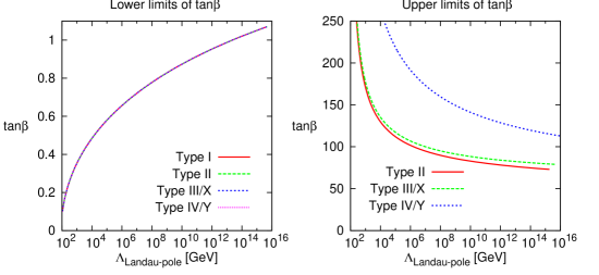
Figure 1: The starting value of tanβ𝛽\tan\beta as a function of the position of the corresponding Landau pole (ΛLandaupolesubscriptΛLandaupole\Lambda_{\rm Landau-pole}) in the different 2HDM types. There are lower limits on tanβ𝛽\tan\beta for all four types (left), but only type II, type III/X and type IV/Y have an upper limit of tanβ𝛽\tan\beta (right).

In Fig. 1 we show the position of the Landau pole as a function of the input tanβ𝛽\tan\beta. For the lower limits, the results are almost the same for all types, and the lines are more or less on top of each other. This is natural since in this regime the evolution is essentially driven by λttsubscript𝜆𝑡𝑡\lambda_{tt}, which is the same in all types. For the upper limits, on the other hand, there are some differences. First of all there is no upper limit on tanβ𝛽\tan\beta in the type I model, which means there is no Landau pole below 1016superscript101610^{16} GeV if the input tanβ>1.1𝛽1.1\tan\beta>1.1. For the other types, the upper limits are shown in the right panel of Fig. 1. The differences can be understood from whether the evolution is driven by λbbsubscript𝜆𝑏𝑏\lambda_{bb} (type III), λττsubscript𝜆𝜏𝜏\lambda_{\tau\tau} (type IV) or both (type II).

4.2 Z2subscript𝑍2Z_{2}-breaking models

Before starting to analyze the Z2subscript𝑍2Z_{2}-breaking models we note that, as shown by Ferreira:2010xe , the Z2subscript𝑍2Z_{2}-symmetry of the RGE’s is still preserved if all the λFsuperscript𝜆𝐹\lambda^{F}’s for the different types are rescaled with a factor x𝑥x for the cotβ𝛽\cot\beta ones and 1/x1𝑥1/x for the tanβ𝛽\tan\beta ones. In addition, when tanβ𝛽\tan\beta is no longer related to the Yukawa couplings it does not have any physical meaning, since it only reflects the basis choice for the general 2HDM. In the following we will only be considering cases with ρ𝜌\rho real at the starting scale. This means that the only source of CP-violation is from the CKM-matrix. Thus the CP-violating effects will be small and therefore the dependence on tanβ𝛽\tan\beta very limited. We have verified this numerically for a number of cases and in the following we set tanβ=1𝛽1\tan\beta=1.

In this subsection, we will also explore the non-diagonal elements of FCNC Yukawa couplings. We know that in the Z2subscript𝑍2Z_{2} symmetric case, the tree level FCNC couplings will remain equal to zero (up to the numerical precision) up to arbitrarily high energy scales since they are protected by the symmetry. However once we break the Z2subscript𝑍2Z_{2} symmetry in some way, this protection is not effective anymore and the off-diagonal elements λijFsubscriptsuperscript𝜆𝐹𝑖𝑗\lambda^{F}_{i\neq j} may start to grow.

The actual values of the non-diagonal FCNC Yukawa couplings ρijFsubscriptsuperscript𝜌𝐹𝑖𝑗\rho^{F}_{i\neq j} at different energy scales will depend on how much we break the Z2subscript𝑍2Z_{2} symmetry. We can thus use the size of the λijFsubscriptsuperscript𝜆𝐹𝑖𝑗\lambda^{F}_{i\neq j} as a measure of how severe different types of Z2subscript𝑍2Z_{2} symmetry breaking are. Of course we do not know how large the λijFsubscriptsuperscript𝜆𝐹𝑖𝑗\lambda^{F}_{i\neq j} can be at higher scales. Still it is reasonable to assume that the values should not be widely different from the ones at the EW scale. Thus we will use a generic value of λijF0.1subscriptsuperscript𝜆𝐹𝑖𝑗0.1\lambda^{F}_{i\neq j}\leq 0.1 as a limit on how much Z2subscript𝑍2Z_{2} symmetry breaking should be allowed and see at which energy scale this limit is reached.

The argument behind this is essentially that we can use the RGE evolution to analyze the stability of the assumptions underlying different 2HDMs under variations of the scale where the model is defined. A large sensitivity indicates that the assumptions behind the model are not stable meaning that they are either fine-tuned or incomplete such that there for example will be additional particles appearing when going to a higher energy. From this respect we will thus study both the appearance of a Landau pole as well as off-diagonal Yukawa couplings leading to FCNC larger than experimentally allowed at the EW scale. We also note that as will become clear below there is a small dependence on at which scale we apply the above argument. Requiring stability up to 103superscript10310^{3} GeV gives very similar constraints on the amount of Z2subscript𝑍2Z_{2}-breaking that is allowed as when using 1015superscript101510^{15} GeV.

As an alternative way of assessing the amount of Z2subscript𝑍2Z_{2}-breaking that is allowed by the experimental constraints from FCNC at the EW scale we have also considered a set-up where the Z2subscript𝑍2Z_{2}-symmetry is broken at a high scale. In this set-up we start from a Z2subscript𝑍2Z_{2}-symmetric model at the EW scale and then evolve it to the high scale of interest. The resulting model is then used as the starting point for exploring different ways of breaking the Z2subscript𝑍2Z_{2} symmetry. Once the Z2subscript𝑍2Z_{2}-breaking has been introduced the different models are then evolved down to the EW scale for comparison with the experimental constraints. We have verified that in representative cases the results obtained in this way are very similar to the first approach and therefore we will not go into any more details.

There are many possibilities to break the Z2subscript𝑍2Z_{2} symmetry and in the following we will consider three ways: aligned, diagonal and non-diagonal λijFsubscriptsuperscript𝜆𝐹𝑖𝑗\lambda^{F}_{ij} as defined below. In most cases we will concentrate on the effects of breaking the symmetry starting from a type I or type II model. The reasons for this is on the one hand that these models are the most well studied cases in the literature and on the other hand that it is in the quark sector that we have the most stringent constraints on the FCNC Yukawa couplings. Thus the breaking of the Z2subscript𝑍2Z_{2} symmetry in the lepton sector will typically have small effects.

In order to be able to separate the effects of breaking the Z2subscript𝑍2Z_{2} symmetry in different ways we will limits ourselves to breaking the symmetry in one specific way at a time.

We start by noting that in the Z2subscript𝑍2Z_{2} symmetric models at least two of the λFsuperscript𝜆𝐹\lambda^{F} are always equal whereas the third one is the same as the other two in type I and the negative inverse of them in the other types. When going to the aligned models we will therefore keep two of the sectors in fulfillment with the Z2subscript𝑍2Z_{2}-symmetry and only break the symmetry through the relation to the third sector. In other words either setting λiiD=λiiLsubscriptsuperscript𝜆𝐷𝑖𝑖subscriptsuperscript𝜆𝐿𝑖𝑖\lambda^{D}_{ii}=\lambda^{L}_{ii}, λiiU=λiiLsubscriptsuperscript𝜆𝑈𝑖𝑖subscriptsuperscript𝜆𝐿𝑖𝑖\lambda^{U}_{ii}=\lambda^{L}_{ii}, or λiiU=λiiDsubscriptsuperscript𝜆𝑈𝑖𝑖subscriptsuperscript𝜆𝐷𝑖𝑖\lambda^{U}_{ii}=\lambda^{D}_{ii} and letting λiiFsubscriptsuperscript𝜆𝐹𝑖𝑖\lambda^{F}_{ii} of the third sector vary independently of the other two.

Another way of breaking the Z2subscript𝑍2Z_{2}-symmetry is by keeping the λijFsubscriptsuperscript𝜆𝐹𝑖𝑗\lambda^{F}_{ij} diagonal but letting the individual diagonal elements be non-equal as has been studied by Mahmoudi and Stål Mahmoudi:2009zx . We will analyze the effects of this type of breaking in the up and down sectors separately again starting from the Z2subscript𝑍2Z_{2}-symmetric cases with either λiiD=λiiL=λttsubscriptsuperscript𝜆𝐷𝑖𝑖subscriptsuperscript𝜆𝐿𝑖𝑖subscript𝜆𝑡𝑡\lambda^{D}_{ii}=\lambda^{L}_{ii}=\lambda_{tt} or λiiD=λiiL=1/λttsubscriptsuperscript𝜆𝐷𝑖𝑖subscriptsuperscript𝜆𝐿𝑖𝑖1subscript𝜆𝑡𝑡\lambda^{D}_{ii}=\lambda^{L}_{ii}=-{1/\lambda_{tt}}. In other words using the type I or II Z2subscript𝑍2Z_{2}-symmetries as starting point.

The third way of breaking the Z2subscript𝑍2Z_{2}-symmetry that we will consider is by setting the non-diagonal elements of λijFsubscriptsuperscript𝜆𝐹𝑖𝑗\lambda^{F}_{ij} nonzero already at the starting scale. Again we will consider setting the up-sector and down-sector non-diagonal elements non-zero separately and apply the type I or type II symmetries for the diagonal elements.

4.2.1 Aligned models

We start by analyzing the three different versions of Aligned models with λUsuperscript𝜆𝑈\lambda^{U}, λDsuperscript𝜆𝐷\lambda^{D}, and λLsuperscript𝜆𝐿\lambda^{L} pairwise equal. Based on the similarities with the Z2subscript𝑍2Z_{2}-symmetric models we call them I/II, III, and IV respectively and their free parameters are as follows

  • Aligned I/II: λiiU,λiiD=λiiLsubscriptsuperscript𝜆𝑈𝑖𝑖subscriptsuperscript𝜆𝐷𝑖𝑖subscriptsuperscript𝜆𝐿𝑖𝑖\lambda^{U}_{ii},\quad\lambda^{D}_{ii}=\lambda^{L}_{ii}

  • Aligned III: λiiD,λiiU=λiiLsubscriptsuperscript𝜆𝐷𝑖𝑖subscriptsuperscript𝜆𝑈𝑖𝑖subscriptsuperscript𝜆𝐿𝑖𝑖\lambda^{D}_{ii},\quad\lambda^{U}_{ii}=\lambda^{L}_{ii}

  • Aligned IV: λiiL,λiiU=λiiDsubscriptsuperscript𝜆𝐿𝑖𝑖subscriptsuperscript𝜆𝑈𝑖𝑖subscriptsuperscript𝜆𝐷𝑖𝑖\lambda^{L}_{ii},\quad\lambda^{U}_{ii}=\lambda^{D}_{ii}

Refer to caption
Refer to caption
Refer to caption
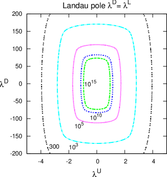
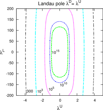
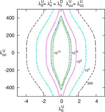
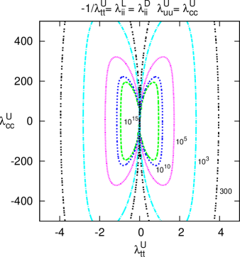
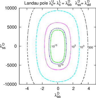
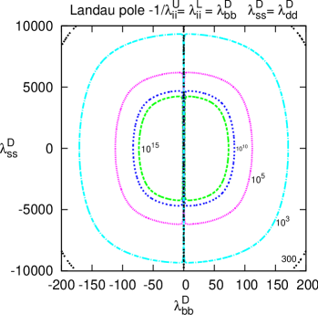
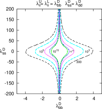
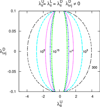
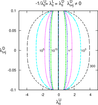
Figure 2: The energy scale at which the Landau pole is encountered as a function of pairwise combinations of the starting values for λiiUsubscriptsuperscript𝜆𝑈𝑖𝑖\lambda^{U}_{ii}, λiiDsubscriptsuperscript𝜆𝐷𝑖𝑖\lambda^{D}_{ii}, and λiiLsubscriptsuperscript𝜆𝐿𝑖𝑖\lambda^{L}_{ii} as indicated in the figure for the three different versions of aligned models explained in the text. The areas inside a given contour are allowed by the requirement of not having a Landau pole. The different contours are as follows starting from the center: 1015superscript101510^{15}, 1010superscript101010^{10}, 105superscript10510^{5}, 103superscript10310^{3}, and 300300300 GeV.

First we consider the effects of requiring that there is no Landau pole encountered when evolving to higher scales. We therefore plot in Fig. 2 the scale at which the Landau pole is reached as a function of the starting values for pairs of λUsuperscript𝜆𝑈\lambda^{U}, λDsuperscript𝜆𝐷\lambda^{D}, and λLsuperscript𝜆𝐿\lambda^{L}. This means that for a given energy scale the points inside the corresponding contour is allowed by this requirement. As can be seen from the figure, the position of the Landau poles is very similar to the situation for the Z2subscript𝑍2Z_{2}-symmetric cases and there is only a small correlation between the values of the aligned Yukawas where the Landau pole is reached.

Refer to caption
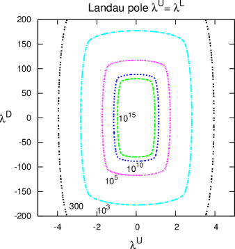
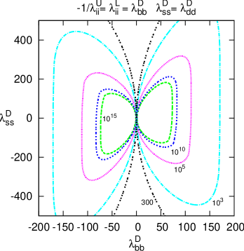
Figure 3: Same as Fig. 2 but also applying the constraints from the non-diagonal λijFsubscriptsuperscript𝜆𝐹𝑖𝑗\lambda^{F}_{i\neq j}. The plot shows the results for λiiL=λiiDsubscriptsuperscript𝜆𝐿𝑖𝑖subscriptsuperscript𝜆𝐷𝑖𝑖\lambda^{L}_{ii}=\lambda^{D}_{ii}, but the same results are also obtained for λiiL=λiiUsubscriptsuperscript𝜆𝐿𝑖𝑖subscriptsuperscript𝜆𝑈𝑖𝑖\lambda^{L}_{ii}=\lambda^{U}_{ii}.

Applying also the condition that the off-diagonal elements of should respect the limits given by the meson mixing constraints also at higher scales has a potentially large impact on the allowed regions. This is the case for the aligned models of type I/II and III, where λLsuperscript𝜆𝐿\lambda^{L} is set equal to λDsuperscript𝜆𝐷\lambda^{D} and λUsuperscript𝜆𝑈\lambda^{U} respectively, as can be seen in Fig. 3. In fact, within the parameter region displayed in the figure (note the difference in scale compared to Fig. 2) there is no difference between the two cases and therefore we only show one of them. However, as may also have been expected, there are no additional constraints in the case when λDsuperscript𝜆𝐷\lambda^{D} and λUsuperscript𝜆𝑈\lambda^{U} are set equal since the off-diagonal lepton Yukawas are always small as a consequence of the small lepton masses and the limited cross-talk between the quarks and leptons. In other words breaking the Z2subscript𝑍2Z_{2} symmetry between the quarks and leptons has no effect in this respect.
Refer to caption
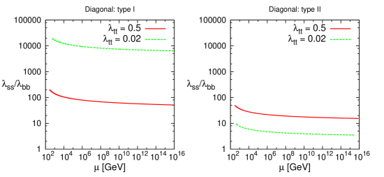
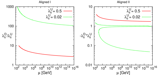
Figure 4: The constraints on the starting values of ξ=λiiD/λiiU𝜉subscriptsuperscript𝜆𝐷𝑖𝑖subscriptsuperscript𝜆𝑈𝑖𝑖\xi=\lambda^{D}_{ii}/\lambda^{U}_{ii} (left) and ξ=λiiDλiiU𝜉subscriptsuperscript𝜆𝐷𝑖𝑖subscriptsuperscript𝜆𝑈𝑖𝑖\xi=-\lambda^{D}_{ii}\lambda^{U}_{ii} (right) as a function of the renormalization scale where the off-diagonal elements reaches 0.1 in the Aligned models of type I and type II respectively for the representative values λiiU=0.02subscriptsuperscript𝜆𝑈𝑖𝑖0.02\lambda^{U}_{ii}=0.02 and 0.50.50.5.

For reference we have also included lines corresponding to the Z2subscript𝑍2Z_{2} symmetric relations in Fig. 3. Along these lines it is the Landau pole that gives the limit but in the other regions the limit comes from the off-diagonal elements. We also note that the plot is symmetric under inversion through the origin (x,y)(x,y)𝑥𝑦𝑥𝑦(x,y)\to(-x,-y), which follows since the evolution equations for ρ0Fsubscriptsuperscript𝜌𝐹0\rho^{F}_{0} are all even under ρ0Fρ0Fsubscriptsuperscript𝜌𝐹0subscriptsuperscript𝜌𝐹0\rho^{F}_{0}\to-\rho^{F}_{0} as long as the imaginary parts of κ0Fsubscriptsuperscript𝜅𝐹0\kappa^{F}_{0} and ρ0Fsubscriptsuperscript𝜌𝐹0\rho^{F}_{0} are small.

It is also interesting to compare the results for non-equal λDsuperscript𝜆𝐷\lambda^{D} and λUsuperscript𝜆𝑈\lambda^{U} with the constraints on λbbsubscript𝜆𝑏𝑏\lambda_{bb} and λttsubscript𝜆𝑡𝑡\lambda_{tt} obtained from bsγ𝑏𝑠𝛾b\to s\gamma in Mahmoudi:2009zx . Applying the conditions of stability when evolving to higher scales and that the non-diagonal Yukawas should stay small essentially removes the regions |λtt|1greater-than-or-equivalent-tosubscript𝜆𝑡𝑡1|\lambda_{tt}|\gtrsim 1 including the fine-tuned regions where λbbsubscript𝜆𝑏𝑏\lambda_{bb} and λttsubscript𝜆𝑡𝑡\lambda_{tt} are both large (2greater-than-or-equivalent-toabsent2\gtrsim 2) and have the same sign.

As special cases we also show in Fig. 4 the results for λiiU=0.02,0.5subscriptsuperscript𝜆𝑈𝑖𝑖0.020.5\lambda^{U}_{ii}=0.02,0.5 and either λiiD=λiiL=ξλiiUsubscriptsuperscript𝜆𝐷𝑖𝑖subscriptsuperscript𝜆𝐿𝑖𝑖𝜉subscriptsuperscript𝜆𝑈𝑖𝑖\lambda^{D}_{ii}=\lambda^{L}_{ii}=\xi\lambda^{U}_{ii} (type I) or λiiD=λiiL=ξ/λiiUsubscriptsuperscript𝜆𝐷𝑖𝑖subscriptsuperscript𝜆𝐿𝑖𝑖𝜉subscriptsuperscript𝜆𝑈𝑖𝑖\lambda^{D}_{ii}=\lambda^{L}_{ii}=-\xi/\lambda^{U}_{ii} (type II). From these plots it is clear that for λiiU=0.5subscriptsuperscript𝜆𝑈𝑖𝑖0.5\lambda^{U}_{ii}=0.5, the off-diagonal elements puts strong constraints on the Z2subscript𝑍2Z_{2}-symmetry breaking parameter ξ=λiiD/λiiU𝜉subscriptsuperscript𝜆𝐷𝑖𝑖subscriptsuperscript𝜆𝑈𝑖𝑖\xi=\lambda^{D}_{ii}/\lambda^{U}_{ii} ( ξ=λiiDλiiU𝜉subscriptsuperscript𝜆𝐷𝑖𝑖subscriptsuperscript𝜆𝑈𝑖𝑖\xi=-\lambda^{D}_{ii}\lambda^{U}_{ii}) with typical values being ξ310(25)less-than-or-similar-to𝜉31025\xi\lesssim 3-10\,(2-5) for type I (II). For λiiU=0.02subscriptsuperscript𝜆𝑈𝑖𝑖0.02\lambda^{U}_{ii}=0.02 on the other hand the constraints are very mild in a type I set-up with ξ1001000less-than-or-similar-to𝜉1001000\xi\lesssim 100-1000 allowed, whereas in a type II setup only ξ𝜉\xi values very close to 1 or ξ0.050.1less-than-or-similar-to𝜉0.050.1\xi\lesssim 0.05-0.1 are allowed. The two possibilities corresponds to two distinct regions in the λiiD,λiiUsubscriptsuperscript𝜆𝐷𝑖𝑖subscriptsuperscript𝜆𝑈𝑖𝑖\lambda^{D}_{ii},\lambda^{U}_{ii} plane. The first one where λiiD1/λiiUsubscriptsuperscript𝜆𝐷𝑖𝑖1subscriptsuperscript𝜆𝑈𝑖𝑖\lambda^{D}_{ii}\approx-1/\lambda^{U}_{ii} and the second one where λiiDsubscriptsuperscript𝜆𝐷𝑖𝑖\lambda^{D}_{ii} is small (25less-than-or-similar-toabsent25\lesssim 2-5). For comparison we recall that the Landau pole constrains λiiD70200less-than-or-similar-tosubscriptsuperscript𝜆𝐷𝑖𝑖70200\lambda^{D}_{ii}\lesssim 70-200 more or less irrespectively of λiiUsubscriptsuperscript𝜆𝑈𝑖𝑖\lambda^{U}_{ii}. So the constraints on ξ𝜉\xi are more or less trivial in this case.

4.2.2 Diagonal models

Next we consider in more detail models with Z2subscript𝑍2Z_{2}-breaking in either the up or the down sector. To make the discussion more clear we only consider models where λttsubscript𝜆𝑡𝑡\lambda_{tt} and λbbsubscript𝜆𝑏𝑏\lambda_{bb} are related in a Z2subscript𝑍2Z_{2} symmetric way and since we have seen that the effects of the lepton sector is small we always set λiiL=λbbsubscriptsuperscript𝜆𝐿𝑖𝑖subscript𝜆𝑏𝑏\lambda^{L}_{ii}=\lambda_{bb}. (If λttsubscript𝜆𝑡𝑡\lambda_{tt} and λbbsubscript𝜆𝑏𝑏\lambda_{bb} are not related in a Z2subscript𝑍2Z_{2} symmetric way then we are more or less back in the aligned models since these two are the dominant Yukawas). In other words we only partially break the alignment.
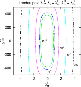
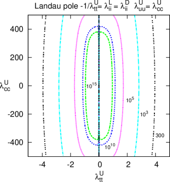
Refer to caption
Refer to caption
Refer to caption
Refer to caption
Figure 5: The energy scale where the Landau pole is reached (upper panels) together with the scale where one of the non-diagonal λijF=0.1subscriptsuperscript𝜆𝐹𝑖𝑗0.1\lambda^{F}_{i\neq j}=0.1 (lower panels) as a function of the input values λccsubscript𝜆𝑐𝑐\lambda_{cc} and λttsubscript𝜆𝑡𝑡\lambda_{tt}. In the left (right) panels λD=λL=λtt(1/λtt)superscript𝜆𝐷superscript𝜆𝐿subscript𝜆𝑡𝑡1subscript𝜆𝑡𝑡\lambda^{D}=\lambda^{L}=\lambda_{tt}(-1/\lambda_{tt}).

Thus we start with considering Z2subscript𝑍2Z_{2}-breaking in the up-sector with λD=λttsuperscript𝜆𝐷subscript𝜆𝑡𝑡\lambda^{D}=\lambda_{tt} (type I) or λD=1/λttsuperscript𝜆𝐷1subscript𝜆𝑡𝑡\lambda^{D}=-1/\lambda_{tt} (type II). For simplicity we also set λuu=λccsubscript𝜆𝑢𝑢subscript𝜆𝑐𝑐\lambda_{uu}=\lambda_{cc}.

First of all, as we show in Fig. 5, the Landau pole gives the restriction λcc400500less-than-or-similar-tosubscript𝜆𝑐𝑐400500\lambda_{cc}\lesssim 400-500 both for type I and II, again more or less independently of the value of λttsubscript𝜆𝑡𝑡\lambda_{tt}. We also want to emphasize that even though it is not really discernable from the figure, there is also a lower limit on λtt0.01greater-than-or-equivalent-tosubscript𝜆𝑡𝑡0.01\lambda_{tt}\gtrsim 0.01 from the Landau pole for λbbsubscript𝜆𝑏𝑏\lambda_{bb} for type II.

The figure also shows that the impact of constraining the off-diagonal elements to be less than 0.1 is limited for the type I set-up. In fact for λtt=0subscript𝜆𝑡𝑡0\lambda_{tt}=0 there is not additional constraint from the off-diagonal elements. In the type II set-up the constraints are more severe but even so quite mild.
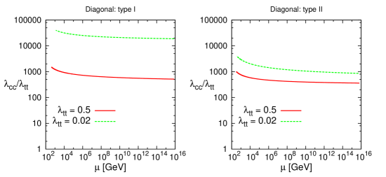
Refer to caption
Figure 6: The constraints on the input values ξ=λcc/λtt𝜉subscript𝜆𝑐𝑐subscript𝜆𝑡𝑡\xi=\lambda_{cc}/\lambda_{tt} as a function of the renormalization scale where the off-diagonal elements reaches 0.1 in the diagonal models of type I (left) and type II (right) for the representative values λtt=0.02subscript𝜆𝑡𝑡0.02\lambda_{tt}=0.02 and 0.50.50.5.

To get a better picture of the range of the amount of Z2subscript𝑍2Z_{2}-breaking allowed we also give in Fig. 6 the constraints on the ratio λcc/λttsubscript𝜆𝑐𝑐subscript𝜆𝑡𝑡\lambda_{cc}/\lambda_{tt} in type I and II set ups for our standard values λtt=0.02subscript𝜆𝑡𝑡0.02\lambda_{tt}=0.02 and 0.50.50.5. From the plots it is clear that this ratio can be as large as 1000similar-toabsent1000\sim 1000 without generating off-diagonal λF0.1superscript𝜆𝐹0.1\lambda^{F}\geq 0.1 all the way up to the GUT scale.

Refer to caption
Refer to caption
Refer to caption
Refer to caption
Figure 7: The energy scale where the Landau pole is reached (upper panels) together with the scale where one of the non-diagonal λijF=0.1subscriptsuperscript𝜆𝐹𝑖𝑗0.1\lambda^{F}_{i\neq j}=0.1 (lower panels) as a function of λsssubscript𝜆𝑠𝑠\lambda_{ss} and λbbsubscript𝜆𝑏𝑏\lambda_{bb}. In the left (right) panels λU=λbb(1/λbb)superscript𝜆𝑈subscript𝜆𝑏𝑏1subscript𝜆𝑏𝑏\lambda^{U}=\lambda_{bb}(-1/\lambda_{bb}) and in all cases λL=λbbsuperscript𝜆𝐿subscript𝜆𝑏𝑏\lambda^{L}=\lambda_{bb}.

Next we consider Z2subscript𝑍2Z_{2}-breaking in the down-sector with λbb=λiiUsubscript𝜆𝑏𝑏subscriptsuperscript𝜆𝑈𝑖𝑖\lambda_{bb}=\lambda^{U}_{ii} (type I) or λbb=1/λiiUsubscript𝜆𝑏𝑏1subscriptsuperscript𝜆𝑈𝑖𝑖\lambda_{bb}=-1/\lambda^{U}_{ii} (type II). Similarly to the up-sector we set λdd=λsssubscript𝜆𝑑𝑑subscript𝜆𝑠𝑠\lambda_{dd}=\lambda_{ss} for simplicity. Also in this case the constraints from the Landau pole are similar for the two set-ups with λss400700less-than-or-similar-tosubscript𝜆𝑠𝑠400700\lambda_{ss}\lesssim 400-700 in both cases with a small correlation with the value of λiiUsubscriptsuperscript𝜆𝑈𝑖𝑖\lambda^{U}_{ii} and λbbsubscript𝜆𝑏𝑏\lambda_{bb} for a set up of type I and type II respectively as can be seen from Fig. 7 (upper panels). However, contrary to the up-sector the figure (lower panels) also shows that the effects from requiring the off-diagonal Yukawas to be small are quite severe. In the type II case one can even see a mild preference for solutions with λssλbbsubscript𝜆𝑠𝑠subscript𝜆𝑏𝑏\lambda_{ss}\approx\lambda_{bb}.

Refer to caption
Figure 8: The constraints on the input values ξ=λss/λbb𝜉subscript𝜆𝑠𝑠subscript𝜆𝑏𝑏\xi=\lambda_{ss}/\lambda_{bb} as a function of the renormalization scale where the off-diagonal elements reaches 0.1 in the diagonal models of type I (left) and type II (right) for the representative values λtt=0.02subscript𝜆𝑡𝑡0.02\lambda_{tt}=0.02 and 0.50.50.5.

To get a more quantitative picture of the constraints we show in Fig. 8 the ratio ξ=λss/λbb𝜉subscript𝜆𝑠𝑠subscript𝜆𝑏𝑏\xi=\lambda_{ss}/\lambda_{bb} for type I and type II using the values λiiU=0.02subscriptsuperscript𝜆𝑈𝑖𝑖0.02\lambda^{U}_{ii}=0.02 and 0.50.50.5. In the type II set-up the constraints are especially restrictive with ξ410less-than-or-similar-to𝜉410\xi\lesssim 4-10 for λiiU=0.02subscriptsuperscript𝜆𝑈𝑖𝑖0.02\lambda^{U}_{ii}=0.02. In the type I set-up the constraints are less severe but even so stronger than the corresponding ones from the up-sector.

4.2.3 Non-diagonal models
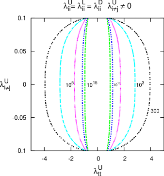
Refer to caption
Refer to caption
Refer to caption
Refer to caption
Figure 9: The constraints from the Landau pole and the off-diagonal elements as a function of λiiUsubscriptsuperscript𝜆𝑈𝑖𝑖\lambda^{U}_{ii} and the off-diagonal elements λijUsubscriptsuperscript𝜆𝑈𝑖𝑗\lambda^{U}_{i\neq j} (up) or λijDsubscriptsuperscript𝜆𝐷𝑖𝑗\lambda^{D}_{i\neq j} (down) at the input scale for the type I (left) and type II (right) relations for the diagonal elements.

Finally we consider the case of breaking the Z2subscript𝑍2Z_{2}-symmetry from having non-zero non-diagonal elements in the up- or down sectors. As starting point we again use the Z2subscript𝑍2Z_{2} symmetric models of type I or II for the diagonal elements and then set either λijU=0.1subscriptsuperscript𝜆𝑈𝑖𝑗0.1\lambda^{U}_{i\neq j}=0.1 or λijD=0.1subscriptsuperscript𝜆𝐷𝑖𝑗0.1\lambda^{D}_{i\neq j}=0.1 at the EW scale in order to break the Z2subscript𝑍2Z_{2} symmetry.

Refer to caption
Refer to caption
Figure 10: Left: The starting value λijUsubscriptsuperscript𝜆𝑈𝑖𝑗\lambda^{U}_{i\neq j} as a function of the energy scale μ𝜇\mu where one of the non-diagonal elements of λijU,Dsubscriptsuperscript𝜆𝑈𝐷𝑖𝑗\lambda^{U,D}_{i\neq j} becomes larger than 0.10.10.1 for λiiU=0.02subscriptsuperscript𝜆𝑈𝑖𝑖0.02\lambda^{U}_{ii}=0.02 and a type II relation between the diagonal elements, λiiD=λiiL=1/λiiUsubscriptsuperscript𝜆𝐷𝑖𝑖subscriptsuperscript𝜆𝐿𝑖𝑖1subscriptsuperscript𝜆𝑈𝑖𝑖\lambda^{D}_{ii}=\lambda^{L}_{ii}=-1/\lambda^{U}_{ii}. Right: The RGE-evolution of the non-diagonal elements λct(μ)subscript𝜆𝑐𝑡𝜇\lambda_{ct}(\mu), λsb(μ)subscript𝜆𝑠𝑏𝜇\lambda_{sb}(\mu), and λdb(μ)subscript𝜆𝑑𝑏𝜇\lambda_{db}(\mu) in the same case for λijU=0.001subscriptsuperscript𝜆𝑈𝑖𝑗0.001\lambda^{U}_{i\neq j}=0.001.

Quite unexpectedly the additional constraints from requiring the off-diagonal elements to stay small are limited. The corresponding plots for the case of only considering the Landau pole are essentially straight vertical lines. Thus we do not show the effects of applying the two constraints separately. In fact it is only in case II with λiiD=λiiL=1/λiiUsubscriptsuperscript𝜆𝐷𝑖𝑖subscriptsuperscript𝜆𝐿𝑖𝑖1subscriptsuperscript𝜆𝑈𝑖𝑖\lambda^{D}_{ii}=\lambda^{L}_{ii}=-1/\lambda^{U}_{ii} and λijU=0.1subscriptsuperscript𝜆𝑈𝑖𝑗0.1\lambda^{U}_{i\neq j}=0.1 that the requirement of having λijU(μ)0.1subscriptsuperscript𝜆𝑈𝑖𝑗𝜇0.1\lambda^{U}_{i\neq j}(\mu)\leq 0.1 gives any discernable effect and then only for small λiiU0.2less-than-or-similar-tosubscriptsuperscript𝜆𝑈𝑖𝑖0.2\lambda^{U}_{ii}\lesssim 0.2. On the other hand, in this case the constraints are very strong as also illustrated in Fig. 10. It is interesting to note that it is actually the off-diagonal elements in the down-sector that become large whereas the ones in the up-sector remain in accord with the limit λijU(μ)0.1subscriptsuperscript𝜆𝑈𝑖𝑗𝜇0.1\lambda^{U}_{i\neq j}(\mu)\leq 0.1. This means that even though there are presently no direct experimental constraints on λctsubscript𝜆𝑐𝑡\lambda_{ct} and λutsubscript𝜆𝑢𝑡\lambda_{ut} they are in this case highly constrained from the link to the down-sector through the RGE evolution. This is then the case in the MSSM, the prime example of a type II 2HDM, for large tanβ𝛽\tan\beta. To see more clearly what happens we show also in Fig. 10 the RGE evolution of the relevant off-diagonal elements for the input values λiiU=0.02subscriptsuperscript𝜆𝑈𝑖𝑖0.02\lambda^{U}_{ii}=0.02 and λijU=0.001subscriptsuperscript𝜆𝑈𝑖𝑗0.001\lambda^{U}_{i\neq j}=0.001, λijD=0subscriptsuperscript𝜆𝐷𝑖𝑗0\lambda^{D}_{i\neq j}=0.

5 Conclusion

We have seen that the RGE evolution is a useful tool to analyze the stability of the assumptions underlying different versions of the 2HDM under variations of the scale where the model is defined. A large sensitivity indicates that the assumptions behind the model are not stable meaning that they are either fine-tuned or incomplete such that there for example will be additional particles appearing when going to a higher energy. From this respect we have studied both the appearance of a Landau pole as well as off-diagonal Yukawa couplings leading to FCNC larger than experimentally allowed at the EW scale.

Based on our studies we have seen that the constraints from avoiding a Landau-pole are in general the same irrespective of the Z2subscript𝑍2Z_{2}-symmetry. They appear as soon as the magnitude of one of the Yukawa couplings becomes of order 1.

The constraints from the off-diagonal elements on the other hand depend on the details of how the Z2subscript𝑍2Z_{2}-symmetry is broken:

  • breaking the Z2subscript𝑍2Z_{2} relation between λDsuperscript𝜆𝐷\lambda^{D} and λUsuperscript𝜆𝑈\lambda^{U} as in the Aligned models is highly constrained with λD/λU10less-than-or-similar-tosuperscript𝜆𝐷superscript𝜆𝑈10\lambda^{D}/\lambda^{U}\lesssim 10 or λDλU10less-than-or-similar-tosuperscript𝜆𝐷superscript𝜆𝑈10-\lambda^{D}\lambda^{U}\lesssim 10 unless λDsuperscript𝜆𝐷\lambda^{D} and λUsuperscript𝜆𝑈\lambda^{U} are both 2less-than-or-similar-toabsent2\lesssim 2,

  • breaking it instead in the up-sector by having λccsubscript𝜆𝑐𝑐\lambda_{cc} and λttsubscript𝜆𝑡𝑡\lambda_{tt} non-equal gives a small difference compared to the constraints coming from the Landau pole with ratios λcc/λtt>1000subscript𝜆𝑐𝑐subscript𝜆𝑡𝑡1000\lambda_{cc}/\lambda_{tt}>1000 allowed,

  • in the down sector the constraints can be much stronger, but also more dependent on the relation between λbbsubscript𝜆𝑏𝑏\lambda_{bb} and λttsubscript𝜆𝑡𝑡\lambda_{tt}, ranging from λss/λbb10less-than-or-similar-tosubscript𝜆𝑠𝑠subscript𝜆𝑏𝑏10\lambda_{ss}/\lambda_{bb}\lesssim 10 for λbb=50subscript𝜆𝑏𝑏50\lambda_{bb}=50 and λtt=0.02subscript𝜆𝑡𝑡0.02\lambda_{tt}=-0.02 to λss/λbb10000less-than-or-similar-tosubscript𝜆𝑠𝑠subscript𝜆𝑏𝑏10000\lambda_{ss}/\lambda_{bb}\lesssim 10000 for λbb=λtt=0.02subscript𝜆𝑏𝑏subscript𝜆𝑡𝑡0.02\lambda_{bb}=\lambda_{tt}=0.02,

  • in the non-diagonal case the constraints are weak when starting from λijD,U=0.1subscriptsuperscript𝜆𝐷𝑈𝑖𝑗0.1\lambda^{D,U}_{i\neq j}=0.1 except in the case λbb=50subscript𝜆𝑏𝑏50\lambda_{bb}=-50 and λtt=0.02subscript𝜆𝑡𝑡0.02\lambda_{tt}=0.02 where we find λijU0.001less-than-or-similar-tosubscriptsuperscript𝜆𝑈𝑖𝑗0.001\lambda^{U}_{i\neq j}\lesssim 0.001. In all cases it is the λijDsubscriptsuperscript𝜆𝐷𝑖𝑗\lambda^{D}_{i\neq j} that become large.

From this we can conclude that starting from a type I Z2subscript𝑍2Z_{2} symmetry there is quite a lot of room for breaking the symmetry as long as one does not encounter a Landau pole except that λD/λU10less-than-or-similar-tosuperscript𝜆𝐷superscript𝜆𝑈10\lambda^{D}/\lambda^{U}\lesssim 10 has to be respected. In the type II case however, the room for breaking the symmetry is much smaller for large λbbsubscript𝜆𝑏𝑏\lambda_{bb}. This is natural since in the latter case κttsubscript𝜅𝑡𝑡\kappa_{tt} and ρbbsubscript𝜌𝑏𝑏\rho_{bb} are both large. It is also interesting to note that this corresponds to the situation in the MSSM with large tanβ𝛽\tan\beta. Finally we conclude that there is little hope to see effects of non-diagonal Yukawa couplings in the top system in a type II model such as MSSM if tanβ𝛽\tan\beta is large.

Acknowledgements

This work is supported in part by the European Community-Research Infrastructure Integrating Activity “Study of Strongly Interacting Matter” (HadronPhysics2, Grant Agreement n. 227431) and the Swedish Research Council grants 621-2008-4074, 621-2008-4219 and 621-2010-3326.

References

  • (1) T. D. Lee, Phys. Rev.  D 8 (1973) 1226.
  • (2) S. L. Glashow, S. Weinberg, Phys. Rev.  D15 (1977) 1958.
  • (3) A. Pich and P. Tuzon, Phys. Rev.  D 80 (2009) 091702 [arXiv:0908.1554].
  • (4) P. M. Ferreira, L. Lavoura and J. P. Silva, Phys. Lett.  B 688 (2010) 341 [arXiv:1001.2561].
  • (5) A. J. Buras, M. V. Carlucci, S. Gori and G. Isidori, JHEP 1010 (2010) 009 [arXiv:1005.5310].
  • (6) C. B. Braeuninger, A. Ibarra and C. Simonetto, Phys. Lett. B 692 (2010) 189 [arXiv:1005.5706].
  • (7) M. Jung, A. Pich and P. Tuzon, JHEP 1011 (2010) 003 [arXiv:1006.0470].
  • (8) F. Mahmoudi, O. Stal, Phys. Rev.  D81 (2010) 035016. [arXiv:0907.1791].
  • (9) T. P. Cheng and M. Sher, Phys. Rev.  D 35 (1987) 3484.
  • (10) G. Cvetic, S. S. Hwang and C. S. Kim, Int. J. Mod. Phys.  A 14, 769 (1999) [arXiv:hep-ph/9706323].
  • (11) G. C. Branco, P. M. Ferreira, L. Lavoura, M. N. Rebelo, M. Sher, J. P. Silva, [arXiv:1106.0034].
  • (12) A. Djouadi, Phys. Rept.  457 (2008) 1 [hep-ph/0503172].
  • (13) A. Djouadi, Phys. Rept.  459 (2008) 1 [hep-ph/0503173].
  • (14) S. Davidson and H. E. Haber, Phys. Rev. D 72 (2005) 035004 [Erratum-ibid. D 72 (2005) 099902] [hep-ph/0504050].
  • (15) R. S. Gupta, J. D. Wells, Phys. Rev.  D81 (2010) 055012. [arXiv:0912.0267].
  • (16) P. M. Ferreira and D. R. T. Jones, JHEP 0908 (2009) 069 [arXiv:0903.2856 [hep-ph]].
  • (17) D. Eriksson, J. Rathsman and O. Stal, Comput. Phys. Commun.  181 (2010) 189 [arXiv:0902.0851 [hep-ph]].
  • (18) H. E. Haber and D. O’Neil, Phys. Rev. D 74 (2006) 015018 [hep-ph/0602242].
  • (19) D. Atwood, L. Reina, A. Soni, Phys. Rev.  D55 (1997) 3156-3176. [hep-ph/9609279].
  • (20) K. Nakamura et al. [ Particle Data Group Collaboration ], J. Phys. G G37, 075021 (2010).
  • (21) J. Laiho, E. Lunghi, R. S. Van de Water, Phys. Rev.  D81 (2010) 034503. [arXiv:0910.2928].
  • (22) E. Lunghi, A. Soni, JHEP 0709 (2007) 053. [arXiv:0707.0212].
  • (23) A. Lenz, U. Nierste, J. Charles, S. Descotes-Genon, A. Jantsch, C. Kaufhold, H. Lacker, S. Monteil et al., Phys. Rev.  D83 (2011) 036004. [arXiv:1008.1593].
  • (24) LHCb collaboration, “Measurement of ΔmsΔsubscript𝑚𝑠\Delta m_{s} in the decay Bs0Ds(K+Kπ)π+subscriptsuperscript𝐵0𝑠superscriptsubscript𝐷𝑠superscript𝐾superscript𝐾superscript𝜋superscript𝜋B^{0}_{s}\to D_{s}^{-}(K^{+}K^{-}\pi^{-})\pi^{+} using opposite-side and same-side flavour tagging algorithms,” LHCb-CONF-2011-050
  • (25) Z. z. Xing, H. Zhang and S. Zhou, Phys. Rev.  D 77 (2008) 113016 [arXiv:0712.1419].
  • (26) G. Guennebaud, B. Jacob et al., http://eigen.tuxfamily.org/
  • (27) M. Galassi, J. Davies, J. Theiler, B. Gough, G. Jungman, P. Alken, M. Booth, F. Rossi ”GNU Scientific Library Reference Manual - Third Edition (v1.12)”, http://www.gnu.org/s/gsl/