Statistics of Stellar Variability from Kepler - I: Revisiting Quarter 1 with an Astrophysically Robust Systematics Correction
We investigate the variability properties of main sequence stars in the first month of Kepler data, using a new astrophysically robust systematics correction. We find that the fraction of stars with variability greater than that of the Sun is 60%, which is marginally consistent with previous studies, and confirm the trend of increasing variability with decreasing effective temperatures. We define low and high variability samples, with a cut corresponding to twice the variability level of the active Sun, and compare the properties of the stars belonging to each sample. We show tentative evidence that the more active stars have lower proper motions and may be located closer to the galactic plane. We also investigate the frequency content of the variability, finding clear evidence for periodic or quasi-periodic behaviour in 16% of stars, and showing that there exist significant differences in the nature of variability between spectral types. Of the periodic objects, most A and F stars have short periods ( days) and highly sinusoidal variability, suggestive of pulsations, whilst G, K and M stars tend to have longer periods ( days, with a trend towards longer periods at later spectral types) and show a mixture of periodic and stochastic variability, indicative of activity. Finally, we use auto-regressive models to characterise the stochastic component of the variability, and show that its typical amplitude and time-scale both increase towards later spectral types, which we interpret as a corresponding increase in the characteristic size and life-time of active regions.
Key Words.:
Techniques: photometric – Stars: activity – Stars: statistics – Stars: rotation1 Introduction
The past decade has seen a rapid increase in the rate of discovery and classification of variable stars, mainly as a result of time-domain photometric surveys whose primary goals were to search for other phenomena, such as microlensing or planetary transits (e.g. the OGLE survey, Udalski et al. 2008). Sources of stellar variability are wide ranging, from the potentially large-amplitude signatures of eclipses, star spots and pulsations, down to the sub-millimagnitude changes induced by granulation. The typical precision and time sampling of ground-based surveys confines the associated variability studies to ‘classical’ variable stars, with amplitudes of a percent or more. In these surveys, the Sun, whose total output never varies by more than around 0.5% peak-to-peak (Fröhlich, 2011), even at the maximum of its activity cycle, would appear as a ‘quiet’ or ‘constant’ star. However, space-based transit surveys such as CoRoT (Baglin, 2003) and Kepler (Borucki et al., 2010) are sensitive to ‘micro-variability’ down to and well below the solar level, on timescales ranging from minutes to months and, over the entire lifetime of Kepler, years.
Measuring the basic characteristics of the variability (amplitude, periodicity, etc…) across large samples of stars, and comparing them to stellar parameters such as age, mass and composition, is a first step towards a better understanding of the underlying phenomena. Many of the latter are ill-understood, because they are related to rotation, convection and magnetism which are challenging to model. Variability statistics also have a crucial impact on exoplanet studies, particularly for radial-velocity searches or radial-velocity confirmation of transiting planet candidates (see e.g. Pont et al., 2011).
Data from the Kepler mission is particularly amenable to statistical variability studies because of the instrument’s unprecedented photometric precision111The Kepler mission requires photometric precision of 20 ppm on 6.5 hr timescales for a Kepler magnitude 12 star, see Jenkins et al. (2010) for a detailed discussion. and vast field of view (115 deg2). The Quarter 1 (Q1) data, which was made public in June 2010, has already been studied by Basri et al. (2010, hereafter B10), who show that somewhat less than half of the dwarf stars surveyed by Kepler are more variable than the Sun on timescales of up to a month, with the fraction increasing from earlier to later spectral types. Basri et al. (2011, hereafter B11) went on to demonstrate that periodic variable stars have significantly larger amplitudes, as a sample, than aperiodic variables. Finally, Ciardi et al. (2011, hereafter C11) performed a complementary study of the same sample using dispersion rather than amplitude as a variability statistic, and studying likely dwarfs and giants separately using the stellar parameters provided in the Kepler Input Catalog (KIC, Brown et al. 2011; Batalha et al. 2010). Variability statistics have also been determined using the 10 days of commissioning data (Q0), with the aim of developing methods to characterise and select specific types of variable (Walkowicz & Basri, 2010).
In C11, the data were corrected for systematics using the Kepler team’s Pre-Search Data Conditioning (PDC) method (Jenkins et al., 2010). This inspired us to investigate further the apparent bimodality in the variability of dwarf stars observed by Kepler, with particular attention to the effect of different systematics correction methods.
The goal of the present paper is to revisit the work of C11 and B10,11 following the application of a new astrophysically robust de-trending method, designed to preserve intrinsic variability signals and remove as fully as possible the systematics. We quantify trends, previously identified and new, between variability characteristics and stellar properties, and investigate the nature of the variability in more detail, in order to gain further insight into the underlying mechanisms.
We describe the data and our systematics correction process in Section 2. In Section 3 we discuss our choice of variability statistics and examine the fractions and physical properties of the low and high variability samples, focussing on their periodic and stochastic nature in Section 4. We present our conclusions and discuss the implications of our findings in Section 5.
2 Systematics Removal in the Q1 Data
2.1 The Data
The Kepler Quarter 1 (Q1) observations took place over 33.5 days between May 13th and June 15th 2009. 156,097 targets were observed during this time, most with a cadence of 29.42 minutes (a small subset were observed with an increased cadence of 1 minute, but only the long cadence data was used in this study). The plate scale is 3.98 arcsec per pixel (van Cleve & Caldwell, 2009) and the astrometric precision for a single 30 minute measure is better than 4 milliarcsec (Monet et al., 2010). Known eclipsing binary systems were removed based on the list compiled by Slawson et al. (2011), available online222http://keplerebs.villanova.edu/. Kepler planet candidates (Borucki et al., 2011) were also removed333http://archive.stsci.edu/kepler/planet_candidates.html. Light curves with discontinuities, detected as a jump greater than and visually confirmed, were also removed, leaving the final sample size at 123030 stars.
Both the ‘raw’ and PDC corrected data are publicly available through the Kepler mission archive444http://archive.stsci.edu/kepler at STScI and also from the NASA Star and Exoplanet Database555http://nsted.ipac.caltech.edu (NStED). This study uses the STScI August 2011 data release. The stellar properties used for classification in this study, namely effective temperature (accurate to 200 K) and surface gravity (accurate to 0.5 dex), come from the KIC. These parameters were estimated using Bayesian posterior probability maximisation to match observed colors, estimated from Sloan g, r, i, z filters, 2MASS JHK, and D51 (510nm), to Castelli & Kurucz (2004) stellar atmosphere models. The proper motion values from the KIC are taken from a selection of catalogs666Kepler Stellar Classification Program, Hipparcos, Tycho-2, UCAC2, 2MASS and USNO-B1.0. where available. Total proper motion is listed on NStED as having accuracy of 20 milliarcseconds per year. 39,000 dwarf stars are listed with non-zero total proper motion. The precisions listed in the KIC are the typical value for each parameter, although in reality these may vary by a small amount between stars of different magnitude and spectral type. For a more detailed discussion of the KIC parameters, see Brown et al. (2011); Batalha et al. (2010); Verner et al. (2011).
2.2 Astrophysically Robust Correction (ARC)
C10 used the PDC corrected flux, whereas B10,11 used the ‘raw’ data, fitting and subtracting a low-order polynomial to remove long-term trends before computing their statistics.
The PDC correction, which is progressively revised and updated, uses ancillary engineering data such as temperature, pointing and focus variations to remove systematic effects from the light curves. The PDC attempts to fit and remove intrinsic variability and then apply the systematics correction to the residuals before re-inserting the stellar signal. This creates a decision point where the program must determine whether the variability is real or not, which can lead to real low amplitude and long term stellar signal being falsely removed. It can also add high-frequency noise (van Cleve, 2010). The polynomial correction of B10,11 can equally affect real long-term variability so we therefore opted to develop a new astrophysically robust correction (ARC) for systematics. The ARC will be presented in detail in a forthcoming paper (Roberts et al. in prep.), but we give a brief outline of it here for completeness.
Our core assumptions are that i) the trends are systematic i.e. they are instrumental in origin and are therefore present, at some level, in the majority of light curves, ii) the underlying number of significant trends is unknown and the trend profile is not pre-specified, iii) the amount of trend present changes from light curve to light curve and is unknown and finally iv) although many trends may be curves with a long timescale, there should be no bias towards smoothness.
We consider the observed set of light curves, , to be composed of a linear combination of underlying “true” curves, , an unknown combination of an unknown number, , of systematic trends, , and an observation noise process, ,
| (1) |
in which the unknown factors represent the amount of trend believed to be present in light curve .
To evaluate the number of trends we start by modelling a light curve, say, as a linear combination of all other curves with factor weights ,
| (2) |
The inference is achieved using a fully Bayesian linear model, based on the computationally efficient variational Bayes methodology and including shrinkage on the parameters.
(a)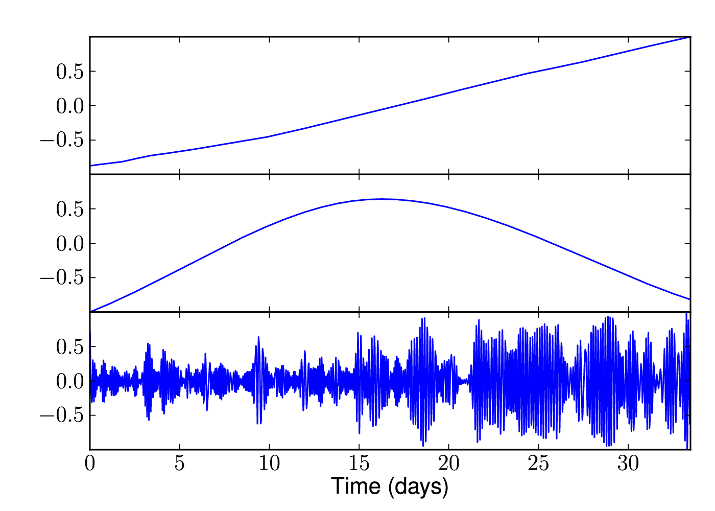 (b)
(b)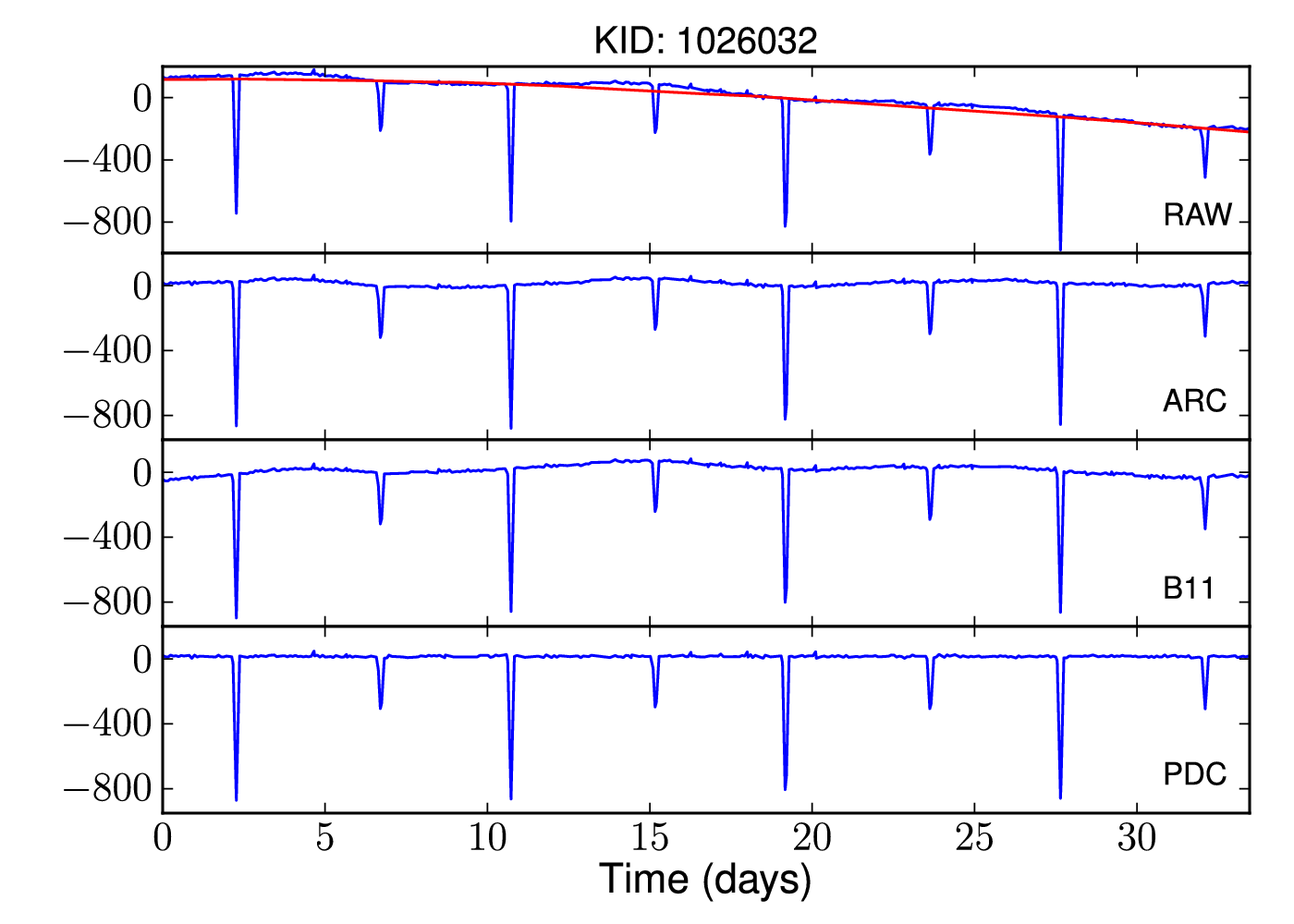
(c)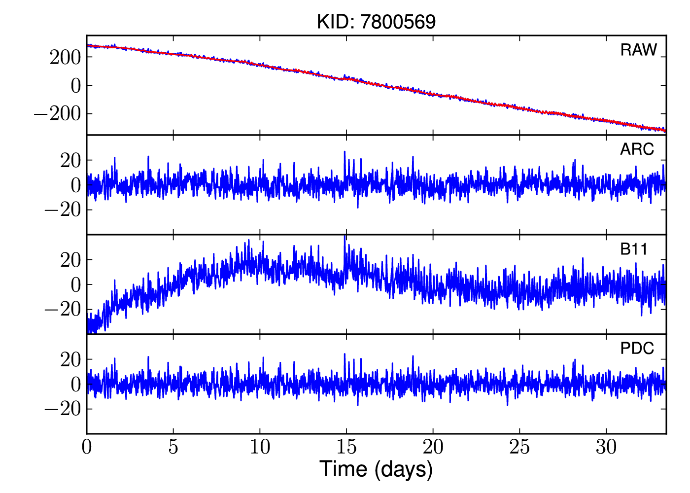 (d)
(d)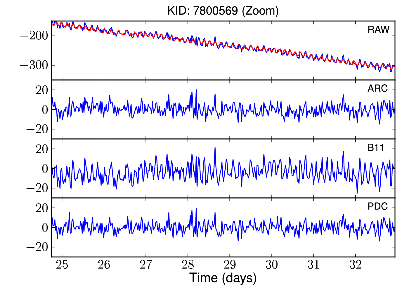
If we consider the inferred empirical distribution of all we expect systematic trends to be associated with the highest entropy distributions - as true systematic trends are more likely to be present in many light curves rather than in just a small subset. Significant777We define significance by considering a principal component analysis of the highest entropy trends and require the first principal component to explain more that 95% of the spectral radius. high-entropy trend components are further processed to remove any residual noise, using empirical mode decomposition (EMD) (Huang et al., 1998), allowing us to recover the dominant dynamic of the trend without imposing any pre-defined smoothness constraints. The latter enables us to extract very low-frequency trends as well as, for example, systematic artefacts due to high frequency vibrations of the satellite. After extraction of the dominant dynamics via EMD, the resultant trend is then removed from all the data by inferring the factors in Equation 1, once again using fully Bayesian inference, giving rise to a modified data set which is deflated with respect to the trend. The entire process of trend discovery and removal is then repeated using the deflated data set until no more significant trends are discovered.
Figure 1(a) shows a typical set of inferred basis trends, obtained from all light curves over all CCDs; note the two typical smooth trends along with the third high frequency vibration effect. Plots (b) and (c) show the raw light curves (blue) along with the inferred trend component (red) and below the de-trended light curves for the different correction methods compared in this paper. Plot (d) highlights a typical section of data in which the high frequency systematic is prevalent and well-removed by the method. These plots demonstrate that the ARC provides the most consistently suitable corrections, removing the high frequency trend in (d), maintaining the true stellar variability in (b) and dealing with low frequency smooth systematics effectively in (c). Comparatively it can be seen that neither the PDC or B10 corrections can perform well in all these areas.
We compared results obtained when correcting all light curves together, with that produced by treating each mod.out888Each module consists of 2 CCDs, which in turn have 2 outputs each. separately. The mod.out separated batches are most suitable since they use the same CCD and channel, which leads to more closely correlated systematics, for example, the reaction motor effects are more prevalent on some CCDs than others.
The ARC performs well in the vast majority of cases, removing systematic trends without altering intrinsic stellar variability signals. One remaining effect that is not currently removed by the ARC is that of the variable guide stars, primarily the eclipsing binary. These introduce small variations in some light curves but these are not frequently occurring or similar enough to be detected by the ARC. A method to detect and remove this effect is currently being devised and will be included in future work, but for this study it may be omitted without significantly reducing the quality of the results.
3 Variability
3.1 Variability Statistics
In order to ensure that we were using the original release of Kepler data correctly, we first reproduced the calculations of B11 as exactly as possible, and compared our results to theirs. We found no discrepancies once the different data reduction methods had been taken into account.
There are a variety of statistics that can be used to quantify variability. The C11 study use the PDC ‘dispersion’ which can be downloaded from (NStED) together with other pre-computed statistics, including the light curve median and reduced . Dispersion is defined as the 1 sigma rms scatter around the median magnitude of the light curve.
Instead of dispersion, B10,11 measured the light curve ‘range’, which is essentially a measure of the peak-to-peak variation. The effect of high-frequency noise was removed either by smoothing the light curve on 10-hour timescales (B10) or by discarding the upper and lower 5 percentiles (B11). The choice of statistic used to study the variability is somewhat arbitrary and we confirm that this choice does not significantly alter the results.
We used the empirical three-section cut of C11 to distinguish between likely dwarfs and giants based on surface gravity and effective temperature , rather than the simpler cut used by B10. It has since been noted that the KIC contains some misidentifications (Koch et al., 2010), but since these are not expected to be numerous enough to affect our results, and for ease of comparison to C11, we used the KIC values without modification.
Based on the method of B11, we have chosen to use the range , between the 5th and 95th percentile, for the median normalised light curve as our variability statistic. Dispersion and reduced provide an appropriate measure of variability that is believed to be primarily stochastic and Gaussian. Pulsations and rotational variability do not meet these criteria and therefore a measurement based on the peak-to-peak variations in the light curve is considered more relevant. Selecting the 5th to 95th percentile range reduces the noise on the peak-to-peak measurement.
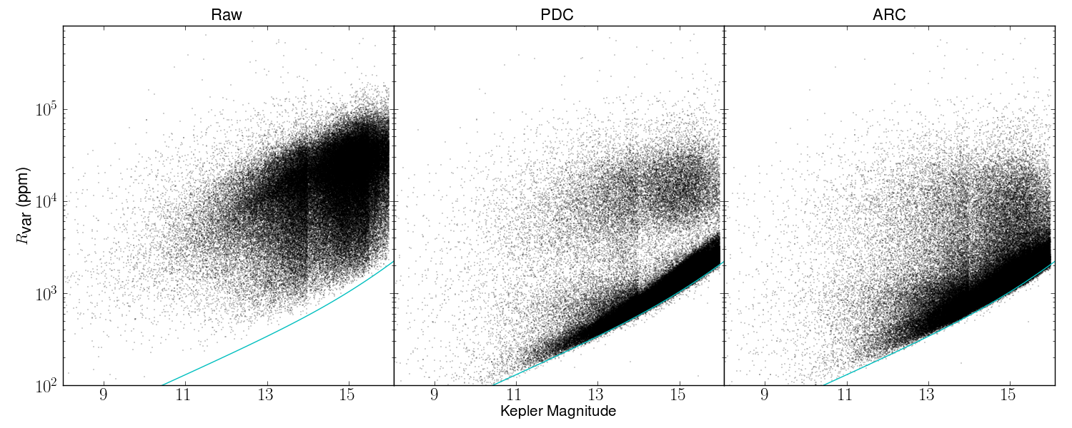
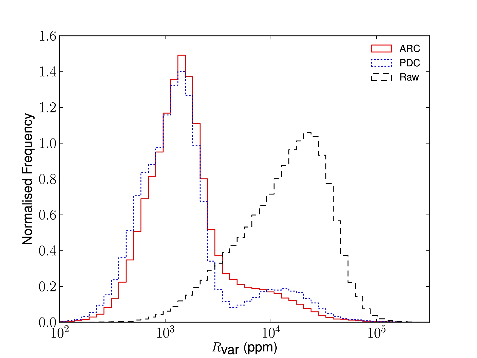
measurements for the Raw, PDC and ARC data are compared in Figures 2 and 3. The ARC clearly removes most systematic effects, reducing the lower envelope of points to the photo noise limit, however it does not have the side effect of suppressing intermediate amplitude variability (as done by the PDC; this is apparent in the scarcity of points around ppm in Figure 3 and the middle panel of Figure 2.) Another unfortunate side effect of the PDC is the introduction of high frequency noise in some light curves, which does not occur with the ARC.
3.2 Solar Comparison and Variability Fraction
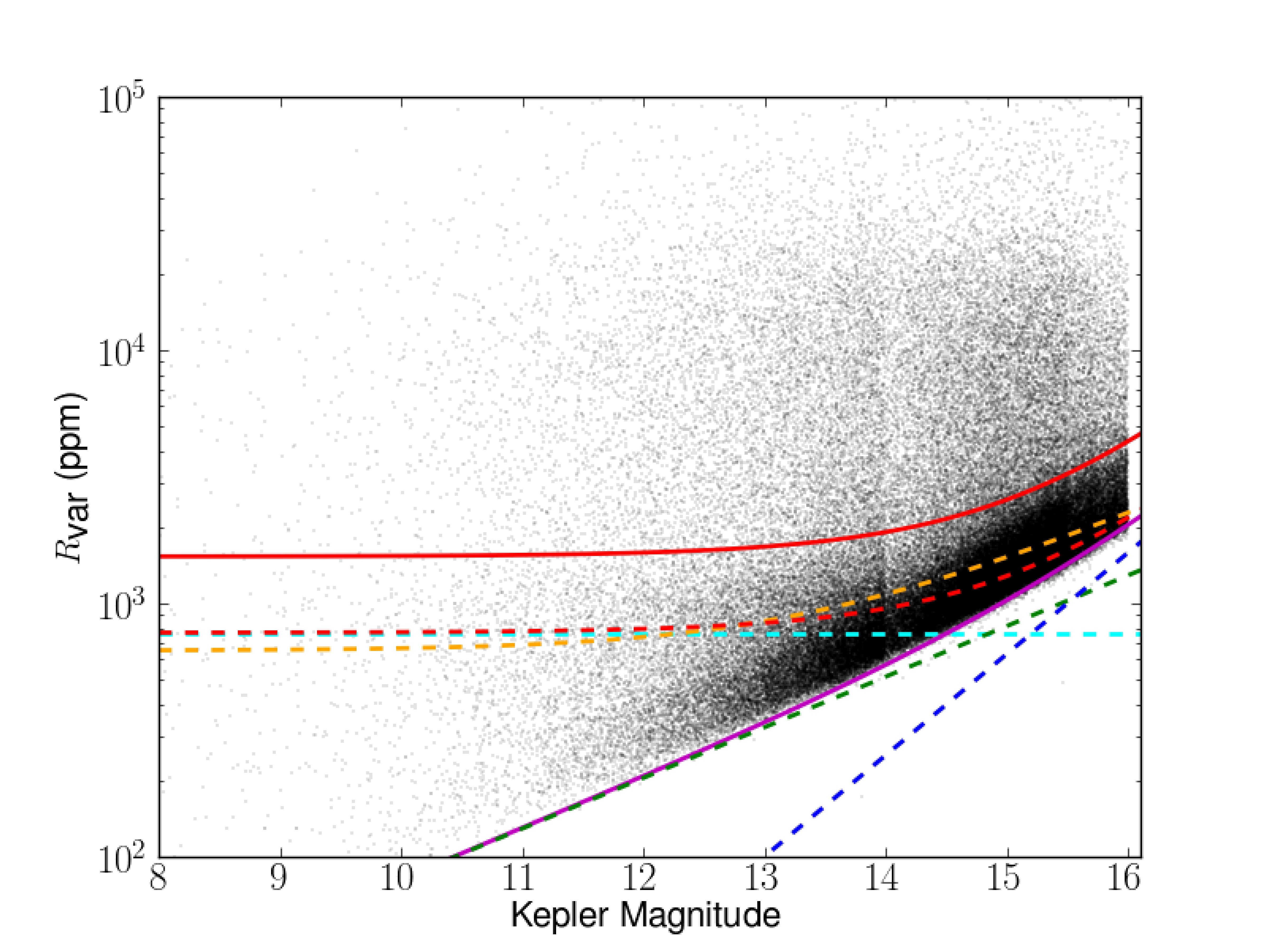
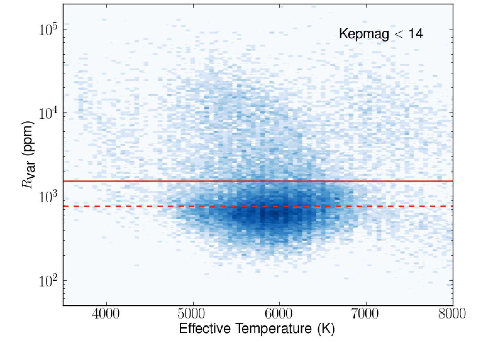
To compare the properties of the high and low variability stars we make a cut in based on a comparison to twice the variability level of the active Sun. This level is somewhat arbitrary but provides an appropriate way to divide stars with approximately solar levels of variability and quieter, from those which are significantly more variable than the active Sun. The solar value was calculated from the SOHO/VIRGO summed g+r light curves for the active Sun in the year 2000, because these provide the closest match to the Kepler bandpass (B10). The solar value was calculated to be 766 ppm from the average obtained using a sliding 33 day section of data over 2 years, centred on the activity maximum. An empirical fit to the median of the photometric uncertainties on the light curves in 0.5 mag bins provides an estimate of noise levels across the range of magnitudes. The equation of the solar equivalent line is composed of the solar measurement, photon and background noise terms,
| (3) |
where best fit values for and are 0.4 and 8.0 respectively. See Figure 4 for a graphical representation of the division process. The orange dashed line in Figure 4 represents the solar line as determined by B10, where extensive visual comparison of solar and Kepler light curves is used to estimate a solar level.
The fractions of dwarf stars with variability greater than the solar level are shown in Table 1. We find that 60% of dwarf stars are more variable than the active Sun on 33 day timescales. B10 find 46% of dwarf stars to be more variable than the solar level. C11 define stars as significantly variable if the reduced is greater than 10, and find the fraction of dwarf stars meeting this criteria to be 18%.
The variability fraction is strongly dependent on the choice and definition of the solar and photometric noise levels. A larger fraction of stars fall into the low variability subset when the division of B10 is used, due to the small difference in the solar value used and more importantly the position of the estimated photometric noise level. Our empirical fit to the median of the photometric uncertainties produces a line that more closely follows the shape of the lower envelope in Figure 4 than the visual estimate of B10.
We calculated the random uncertainty for each of the variability and periodicity fractions listed in Table 1 by performing 10,000 measurements using random samples of 80% of the data, and found these to be < 0.5% and hence negligible in comparison to difference introduced by the choice of dividing line.
It is important to note that for many stars in the low variability sample, the lower limit of is due to the photometric precision of the Kepler satellite, shown as the magenta line in Figure 4. However, due to the position of the dividing line (solid red line in Figure 4) and its dependence on the photometric precision, there are still a large number of stars that are significantly more variable than the photometric noise limit for their magnitude. There are 1,500 stars in the low variability sample that are above twice the photometric noise level.
| Sample | > Solar | > 2Solar | Periodic Fraction |
|---|---|---|---|
| All Dwarfs | 0.60 | 0.20 | 0.16 |
| A | 0.53 | 0.42 | 0.23 |
| F | 0.46 | 0.15 | 0.17 |
| G | 0.56 | 0.14 | 0.13 |
| K | 0.79 | 0.33 | 0.20 |
| M | 0.96 | 0.56 | 0.25 |
3.3 Comparison of Low and High Variability Stellar Properties
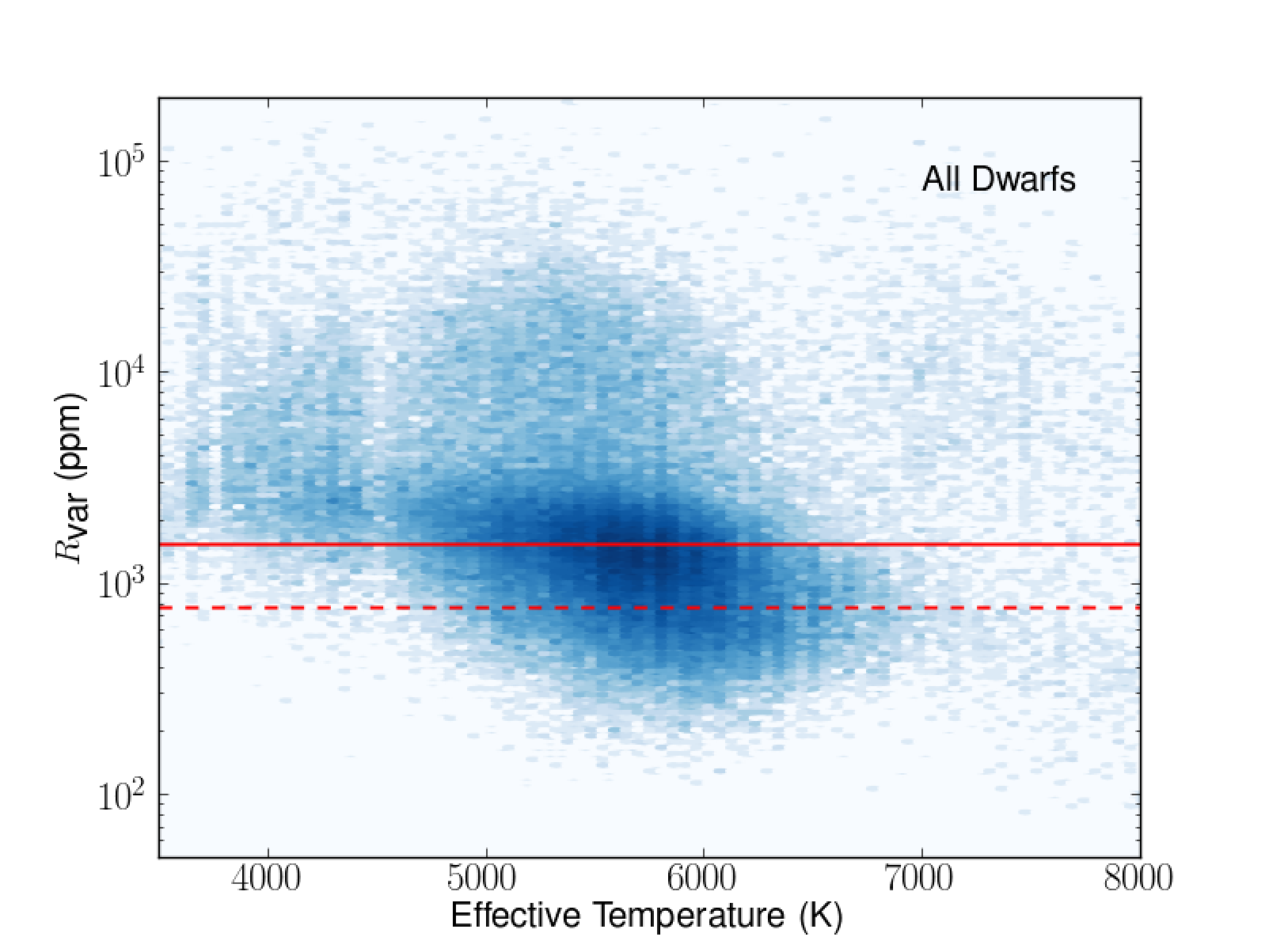
B10,11 and C11 highlighted various relationships between variability and stellar properties. We revisit these using the ARC data. As C11 noted, there is a decrease in variability with temperature which cannot be entirely explained by the increased noise levels in the fainter cool stars (see Figure 5). Pearson’s correlation coefficient of effective temperature and for the whole dwarf sample is -0.31.
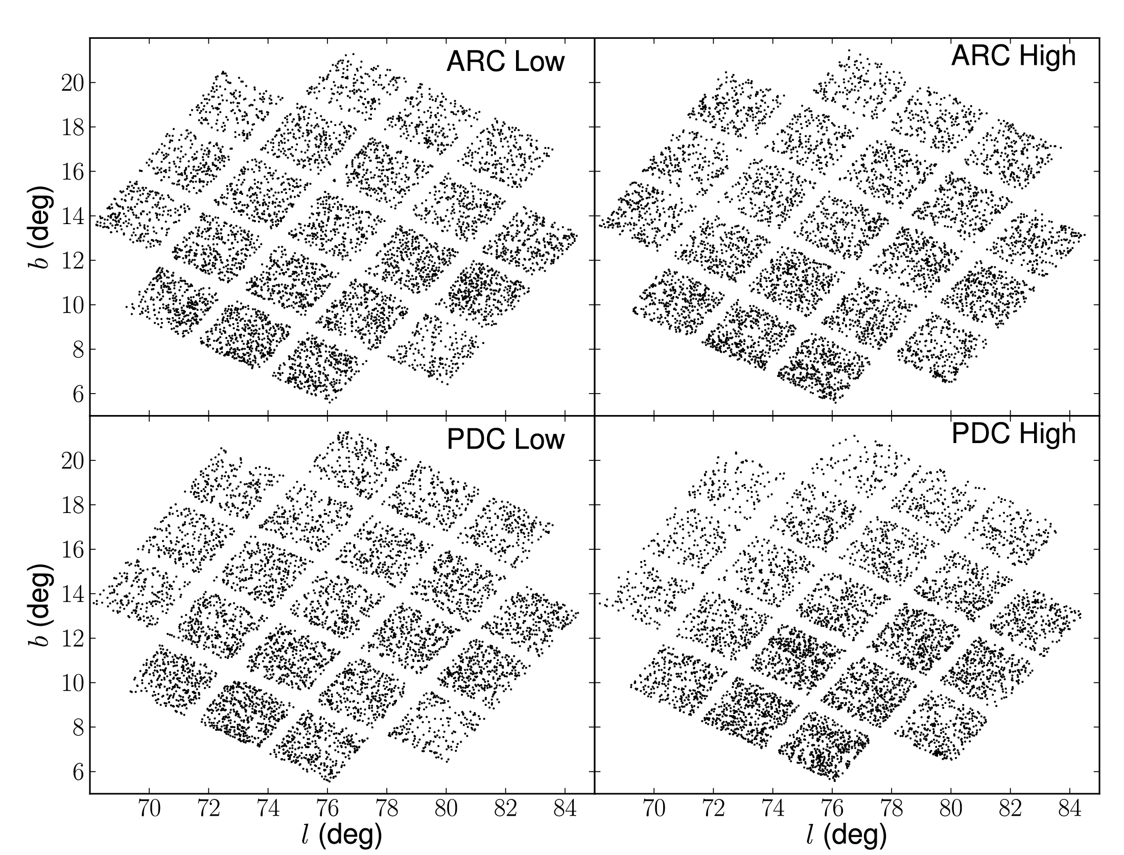
To examine whether the high and low variability samples belong to different stellar populations, we investigated the possible differences in their spatial distribution and kinematics. Due to dynamical heating of the galactic disk over long timescales, older populations of stars tend to have larger galactic scale heights and larger velocity dispersions than younger populations (see e.g. Freeman & Bland-Hawthorn, 2002, and references therein). We therefore examined the distribution of the two samples in galactic coordinates, which is shown in Figure 7.
The division in introduces a magnitude bias between the high and low samples, with a greater proportion of the low variability objects at higher magnitudes. To reduce any possible effect of this bias on our comparison tests, we selected high and low variability subsets with approximately equal magnitude distributions. This was done by dividing the stars into 1 mag bins (with the exception of stars brighter than 8th and fainter than 16th in Kepler magnitude, which were treated separately), and choosing a random set from the more populated bin to match the number in the smaller one. This process, used for the spatial distribution and proper motion comparison tests, also serves to select an equal number of stars in the high and low variability sets.
When using the PDC data, a difference in spatial distribution of the two subsets is evident, as noted by C11. The low variability stars appear approximately uniformly distributed, whereas the high variability stars are concentrated towards low galactic latitudes. Using the PDC data alone, one could hypothesise that the variable sample may correspond to a younger, thin disk population, and the quiet sample to an older population with larger scale height. C11 hinted at this conclusion but argued that this could also be an artefact of increased crowding at low galactic latitudes, causing higher levels of photometric dispersion.
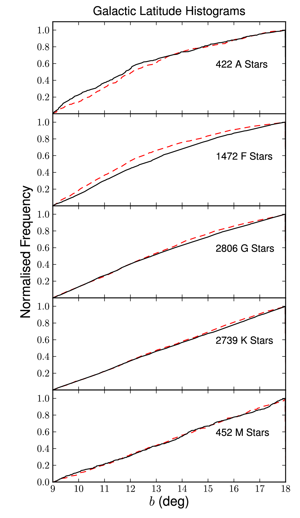
By visually comparing the spatial distribution of the high and low variability samples from the PDC and ARC, it becomes evident that the effect is dependant on the choice of reduction method (Figure 7). This suggests that contamination effects were the dominant cause of the apparent higher variability close to the galactic plane, and that the ARC is better at removing the associated systematics. There is still some sign that active F stars are more concentrated at lower latitudes (Figure 8), but it is too subtle to draw any strong conclusions.
The giant contamination in the F stars is higher than other spectral classes because they span the temperature range where the giant branch intersects the main sequence on the HR diagram. This may lead to the apparent concentration of variable F stars at low galactic latitudes, if the variable and luminous giants are visible out to greater distances in the galactic plane, and hence appear with higher density in these regions.
We also performed a more quantitative two-sample Kolmogorov-Smirnov (KS) test. The results are shown in Table 2, and confirm that the galactic latitudes of the low and high variability F stars are very unlikely to be drawn from the same distribution, compared to a high probability for the M stars. The distribution shape parameters, also shown in Table 2, display the trends of increasing median galactic latitude with later spectral type and the subtle differences between high and low variability subsets, although these are not sufficient to prove the stars belong to different populations. The spatial distribution plots also serve to show that the correction applied using ARC affects all areas of the CCD equally, despite being implemented on each mod.out separately.
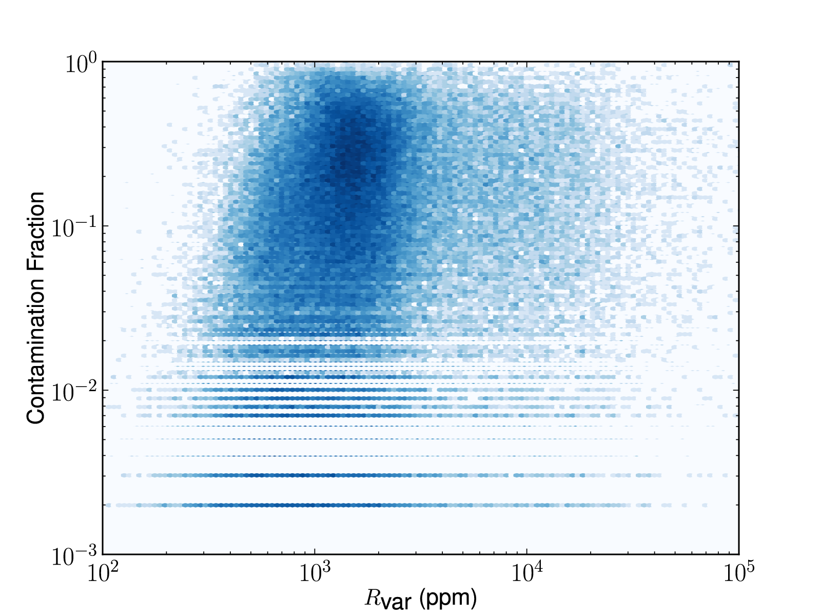
To examine the effect of crowding, we used the contamination fraction available from the Kepler mission archive, which provides an approximate measure of the fraction of flux attributed to the target in a 21 21 pixel aperture. Values range from 0, implying no contamination, to 1, which indicates the flux is essentially all background. There is a weak correlation between contamination fraction and , shown in Figure 9. We tested whether placing a constraint on the contamination fraction, using only targets in the range 0.1 to 0.2, altered the appearance of Figure 7, but it did not.
| Sample | KS | Med L | Med H | MAD L | MAD H | Skew L | Skew H |
|---|---|---|---|---|---|---|---|
| A | 0.016 | 11.68 | 12.00 | 1.76 | 1.57 | 0.70 | 0.54 |
| F | 1.4 | 12.52 | 11.79 | 1.92 | 1.70 | 0.35 | 0.59 |
| G | 0.002 | 12.88 | 12.65 | 2.08 | 1.95 | 0.21 | 0.28 |
| K | 0.1 | 13.29 | 13.32 | 2.21 | 2.08 | 0.07 | 0.04 |
| M | 1.0 | 13.65 | 13.58 | 2.21 | 2.08 | -0.004 | -0.016 |
| Sample | KS | Med L | Med H | MAD L | MAD H | Skew L | Skew H |
|---|---|---|---|---|---|---|---|
| A | 0.61 | 0.0057 | 0.0063 | 0.0032 | 0.0030 | 4.61 | 1.57 |
| F | 0.09 | 0.0077 | 0.0076 | 0.0038 | 0.0033 | 9.57 | 12.66 |
| G | 0.0009 | 0.010 | 0.0091 | 0.0045 | 0.0037 | 12.06 | 4.45 |
| K | 0.002 | 0.013 | 0.011 | 0.0061 | 0.0045 | 8.75 | 9.41 |
| M | 1.5 | 0.033 | 0.020 | 0.013 | 0.0091 | 2.41 | 4.48 |
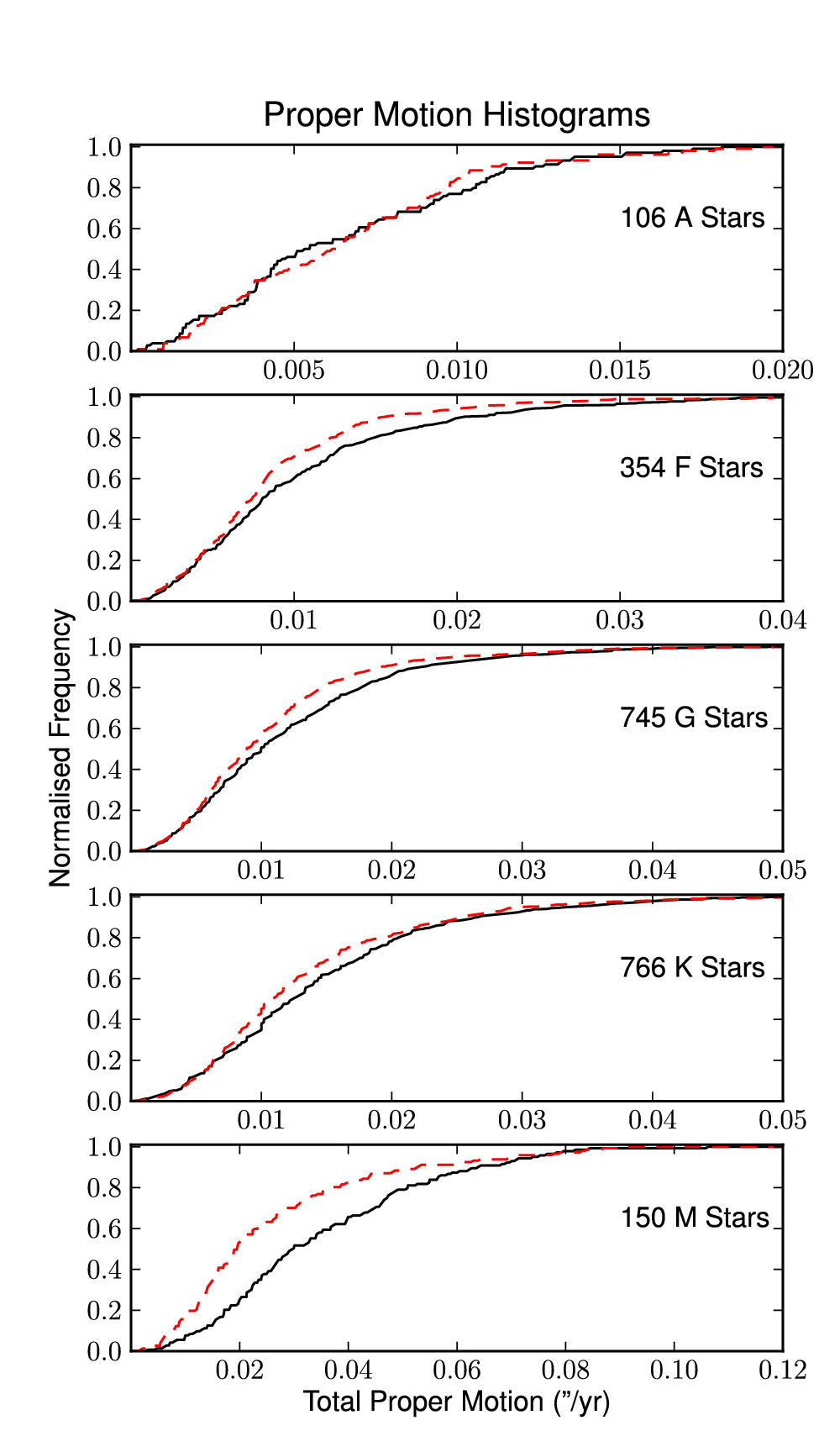
A potential indication that the low and high variability subsets belong to different stellar populations can be seen in the proper motion distributions (Figure 10), for stars with total proper motion greater than zero. It shows a weak but noteworthy trend for the high variability group to have lower proper motion than the low variability group. We also tested the significance of these differences using two-sample KS tests, and parameterised the shape of the distributions, the results of which can be seen in Table 3. The KS test results show that with the exception of A stars, and to some extent F, the proper motion values for the high and low variability groups are very unlikely to be drawn from the same distribution, while the shape parameters highlight more subtle differences in shape and trends between spectral types. This is consistent with the view that higher variability stars are younger and therefore have lower proper motions. This conclusion is dependant on the stars being at the same distance and location on the sky. In our samples, the magnitude and spatial distributions are approximately equal for the high and low variability subsets, which should satisfy this condition. One caveat applicable to the proper motion distributions is that the giant contamination in the M dwarfs (described by C10) could increase the apparent number of high variability stars with low proper motion. We have also considered potential effects of Malmquist bias in our results, but believe that by selecting equal magnitude distributions and comparing each spectral type separately, any effect introduced should be negligible.
4 Periodic and Stochastic Variability
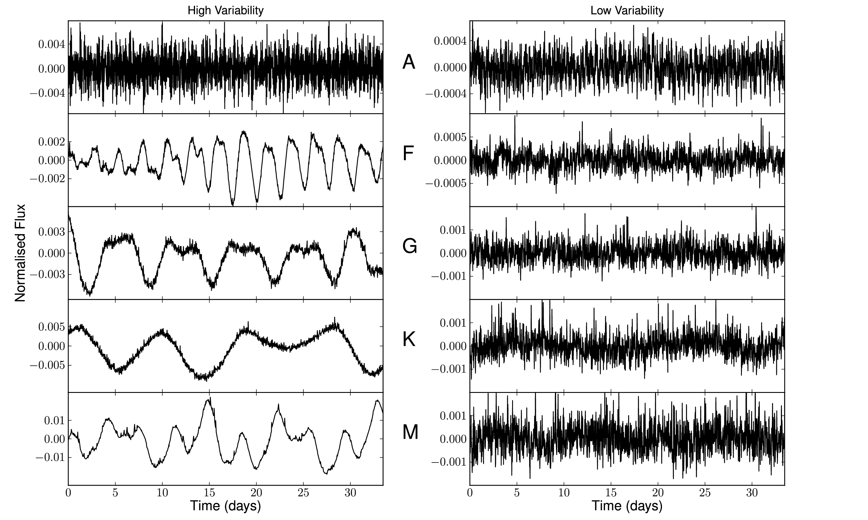
We investigated the nature of the variability, comparing the low and high variability samples, using a combination of visual examination, the statistics described in Section 3, and periodogram analysis. The typical characteristics of the light curves also vary between spectral types as shown in the examples in Figure 6. Visual examination of the light curves shows that A and F stars contain many pulsators with a large range of amplitudes, while later types show rotational modulation and more stochastic variability. This trend is also apparent in the periodicity and stochasticity tests described in this section.
4.1 Periodicity
For each light curve, we computed a periodogram by least-squares fitting of a sinusoid plus a constant at each trial period. The periodogram is expressed in terms of the statistic
| (4) |
where is the reduced chi-squared of the light curve with respect to a constant value, and is the reduced chi-squared with respect to the best-fit sinusoid. We used 500 logarithmically-spaced periods between 0.01 and 100 days. However, only periods between 1 hour (twice the sampling rate) and 16 days (half the time span of the data) were considered valid. We chose this approach over limiting the initial search space to this range, because this would have led to many spurious detections close to the upper limit. Note that some objects with true periods above 16 days may be detected at harmonics of their true period.
The dearth of stars with periods detected close to the 16 day limit is a bias introduced by the stringent period identification method. Many objects that would occupy this period range have broad periodogram peaks at around the 16 day limit and the selection method has been designed to only accept periodogram peaks that drop to the median level before reaching the edges of the allowed range. This prevents false detections of periods at the length of the permitted dataset, and misidentification of the highest periodogram continuum point as a genuine peak.
Bretthorst (1998) describes the Bayesian theory of modelling data using a sinusoid plus white noise. In this formalism, our metric can be shown to be
| (5) |
| (6) |
is the squared magnitude of the discrete Fourier transform of the data. is the number of data points in the light curve, , and is the rms scatter of the data. We have assumed the data is mean-subtracted.
As discussed in B11, the choice of a threshold for periodicity detection is best made empirically. We selected as an appropriate threshold between clear-cut periodic variability and non-periodic or ambiguous cases. This threshold is slightly lower than the value of used in the Monitor project (see e.g. Irwin et al., 2006), which is reasonable given the vastly superior time-sampling of the Kepler data.
This threshold can be compared to a power spectrum cut, since the power spectrum is given by where, following Kjeldsen & Bedding (1995) we have normalised the power spectra such that a sinusoidal oscillation of amplitude gives rise to a peak of height in the power spectrum. Our threshold is then equivalent to a power spectrum threshold of . By comparison Kjeldsen & Bedding (1995) give an expression for the noise level in the power spectrum of .
In our data, , so our threshold is conservative when comparing to white noise. However, white noise is not the dominant factor defining our ability to detect periodicities. To test the appropriateness of our periodicity threshold on data with realistic noise properties, we ran a set of simulations where we injected periodic signals into actual Kepler light curves. We randomly selected 1000 Q1 light curves with low variability () and no significant period (), and injected sinusoidal signals into them, with random periods uniformly distributed between 2 and 16 days, and random amplitudes ranging from 0.1 to 10 times the high-frequency noise level (measured as the scatter in the difference between consecutive flux measurements), with a distribution of amplitudes relative to the noise level that was uniform in log. We then stored the best-fit value of and the corresponding period. We found that was always when the best-fit period differed by from the injected value, suggesting a false detection rate . As one would expect, the missed detection rate is period- and amplitude-dependent: there were only 5 cases in our simulations where the recovered period was within of the injected one but was , and these were all for days and amplitudes significantly smaller than the noise. However, our simulations did not include a large enough number of these low-amplitude, difficult to detect signals to make a more detailed estimate of the completeness. Since the period search in Q1 data was intended as a preliminary exercise, and the results will become much more reliable when additional data is included, we decided additional simulations were beyond the scope of the present paper.
Using the criteria outlined here, 16% of the dwarf stars are determined to be periodic, and the fraction for each spectral type is given in Table 1. We note that these numbers vary slightly from those quoted in B11 and C11. This indicates that our threshold for periodicity is more stringent, designed to detect only genuine periodicities (or strong harmonics) within the limits of the frequency resolution. The periodic fraction will undoubtably increase with longer datasets and more efficient quasi-periodic signal detection methods.
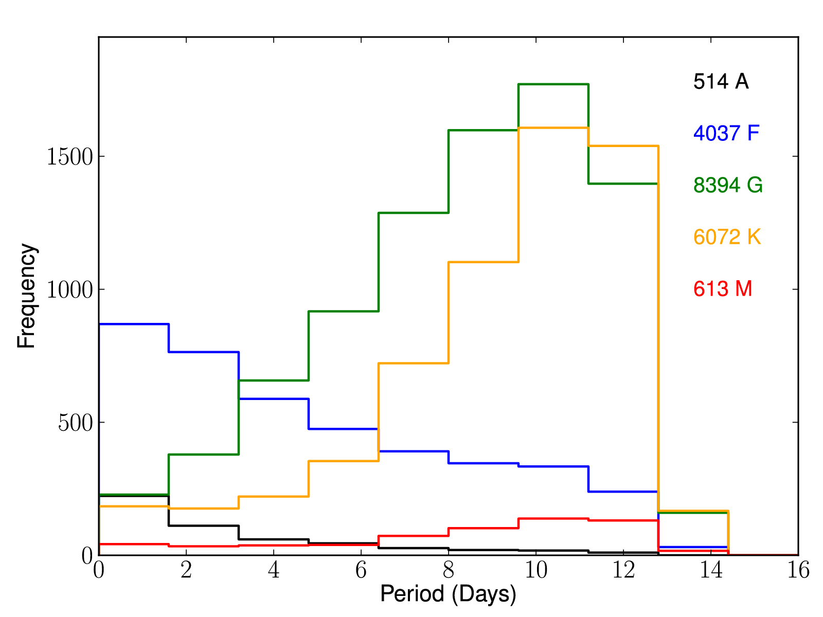
Histograms of the detected periods for each spectral class are shown Figure 11. When interpreting these, one should bear in mind that our period sensitivity is non-uniform, and that the largest peak in the periodogram is not necessarily at the true period but can be at one of its harmonics. The distribution is also truncated close to the maximum period due to the definition of ‘peak’ required for selection. These period distributions should thus be taken as indicative only (the period sensitivity will improve vastly with longer time coverage). Nonetheless, differences between the histograms are obvious, with the typical period clearly increasing towards later spectral types.
The majority of A stars, and about half of F stars, have very short periods ( days). These are likely to be pulsators (many of the A and F stars are located in the instability strip), although they could also be unpublished close binaries (where ellipsoidal variations and mutual heating induce sinusoidal variations) or active stars with very short rotation periods. On the other hand, G, K and M stars, along with the rest of the F stars, have significantly longer periods ( days), as one might expect from rotational modulation of active regions. This distinction is confirmed by the appearance of the light curves (Figure 6). The trend of longer periods towards later spectral types is also visible amongst the late type objects.
4.2 Degree of Stochasticity
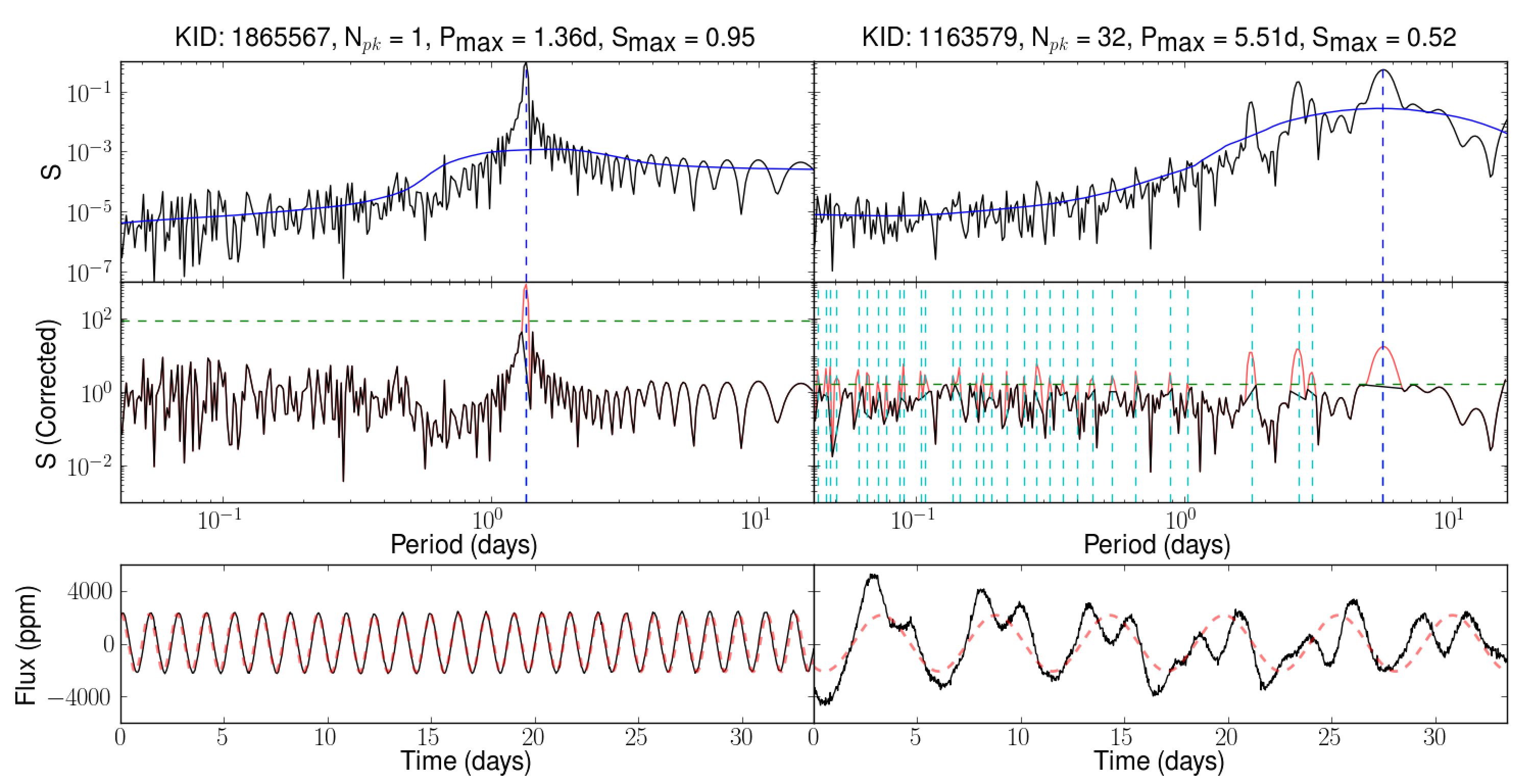
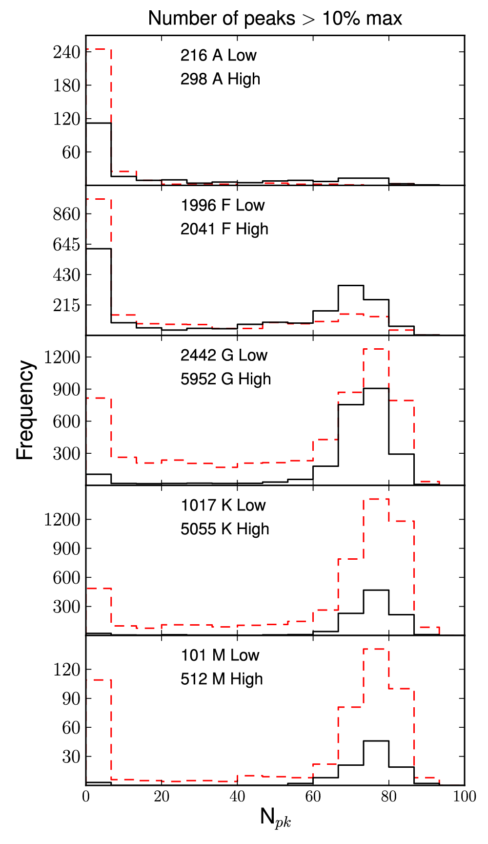
A significant difference in the nature of variability across different spectral types is shown by the degree of stochasticity. We performed a simple measure of this based on the number of peaks, , in the sine-fitting periodogram which have power greater than 10% the maximum power. We selected only stars above the periodicity threshold described in Section 4.1. An example determination is shown in Figure 12.
The histograms showing the distribution for each spectral type are displayed in Figure 13. The light curves of pulsating stars are dominated by near-sinusoidal variability at one, or a few, clear dominant periodicities, corresponding to low values of . Rotational variables are less well modelled by sine-fitting. They typically have a more complex periodogram, with significant power at multiple harmonics of the dominant period (see e.g. Boisse et al., 2009) and some stochastic variability (with power at all frequencies, as seen in the case of the Sun, see e.g. Aigrain et al. 2004). This results in somewhat larger values of . The high variability group show a tendency towards slightly lower levels of stochasticity than the low variability group, which may arise from the strongly periodic pulsating stars that typically have high amplitude variations. It is important to note that the statistic is not a quantitive measure of stochasticity, but intended for use as a comparison between the low and high dispersion samples.
Alternative metrics for measuring timescale, periodicity and stochasticity were demonstrated by Walkowicz & Basri (2010), who use time separation between points where the differential light curve crosses zero, and the time separation between changes in the sign of the slope in the light curve. This method, without smoothing of the light curve, is slightly more sensitive to noise than the approach.
4.3 Harvey Model Fitting
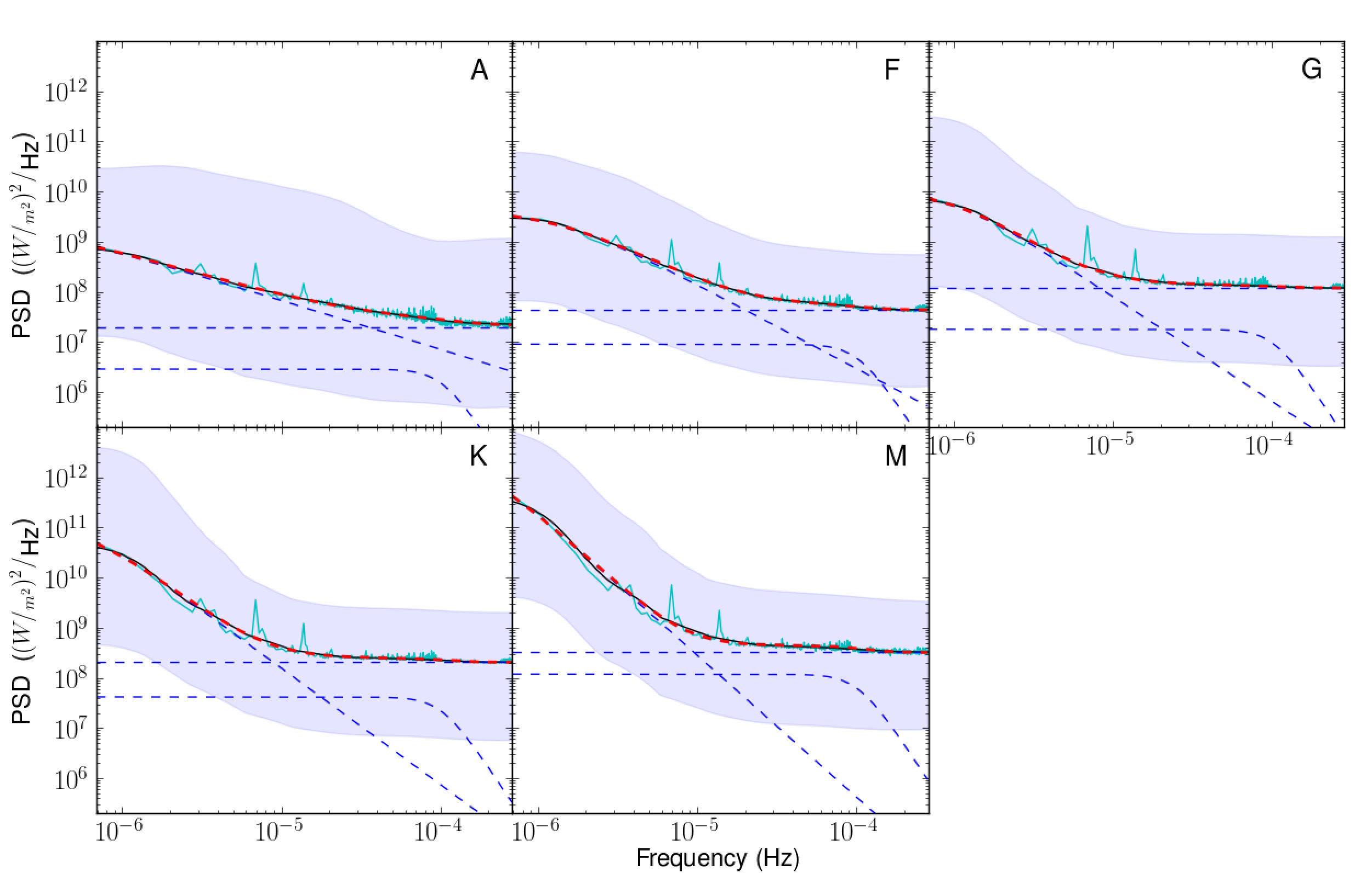
We also studied the typical stochastic properties of each spectral class by fitting a model to the average power spectra of each. The Fast Fourier Transform (FFT) of each light curve was computed and the median, 10th and 90th percentile at each frequency were used to create the plots in Figure 14. These spectra were smoothed using a nonlinear median boxcar filter to remove the effects introduced by the variable pointing stars (evidence of which can be seen in the peaks of the cyan line in Figure 14).
Autoregressive (AR) models are commonly used to describe stochastic processes and take the form,
| (7) |
where and are data values at time index and - respectively, is a constant, is the order of the model, are the parameters and is white noise. Such a process has a spectral density
| (8) |
where is frequency, is the amplitude of the th component, is its characteristic timescale, and is the slope of the power law. By considering the power spectra as a sum of different AR(1) spectra, one can fit a model of this form, first introduced by Harvey (1985) and previously used to model stellar spectra (see e.g. Aigrain et al., 2004; Michel et al., 2009).
The Harvey model consists of a constant background level, a component to describe the intrinsic power at each frequency, and a second component to describe the extra power at Hz introduced by the onboard motor vibrations. The timescale and slope of the motor component have been set to the mean value found when the parameters are allowed to vary, because there is no reason they should be different between spectral types. The amplitude for each is allowed to vary because it will have a greater effect for the fainter stars.
The median power spectrum and fitted powerlaw models describe the typical stochastic background variability of the stars. Clear trends through the spectral classes can be seen in the fit parameters, listed in Table 4. As expected, the background constant increases steadily towards the fainter classes. The amplitude, timescale and slope of the powerlaw fit also increases towards later spectral types. This may arise from the slower typical rotation periods associated with later type stars, creating large, slowly evolving active regions. The timescale of the A stars does not fit this trend, which is most likely due to the large number of pulsating stars shifting the median power towards slightly longer timescales, and the fact that the frequency resolution is not sufficient to resolve the powerlaw turnoff.
| SpT | Background | ||||||
|---|---|---|---|---|---|---|---|
| A | 1.9e7 | 4.1e9 | 1.0e6 | 1.0 | 2.9e6 | 1.6e3 | 4.8 |
| F | 4.3e7 | 4.3e9 | 1.2e5 | 1.7 | 9.1e6 | 1.6e3 | 4.8 |
| G | 1.2e8 | 1.1e10 | 1.6e5 | 2.1 | 1.8e7 | 1.6e3 | 4.8 |
| K | 2.0e8 | 1.2e11 | 2.8e5 | 2.3 | 4.2e7 | 1.6e3 | 4.8 |
| M | 3.2e8 | 1.9e12 | 3.6e5 | 2.8 | 1.2e8 | 1.6e3 | 4.8 |
5 Discussion and Conclusions
We have developed an astrophysically robust systematics correction method (ARC), which has been shown to remove the significant systematic trends from the Kepler Q1 light curves, while maintaining intrinsic stellar variability. Figure 2 shows that the ARC performs to the same standard as the PDC in reducing the lower envelope of the measured variability down to the photometric uncertainty. Crucially, unlike the PDC it does not remove real astrophysical signatures (predominantly at medium variability levels), leading to the apparent bimodality in variability level that can be seen in the PDC panel of Figure 2. The correction is applied individually to each mod.out but the results are shown to be consistent across the whole field of view (Figure 7).
Following B11, we quantified the variability level of each star as the interval between the 5th and 95th percentile of its light curve, and we focused our study on the main-sequence stars, separating them from giants using the -dependent cut defined by C10. A division between low and high variability was made using a magnitude dependent cut in at twice the equivalent variability measurement for the active Sun, resulting in a split of 80% low and 20% high. We examined the relationship between the nature of the variability and physical properties of the stars, and compared our work to that of C11, who use the PDC data and B10,11, who use a polynomial fitting correction method. As suggested by B10 and C11, we see clear evidence for a decrease in variability with increasing temperature (Figure 5), which cannot be entirely explained by selection effects or the noise floor at fainter magnitudes. This is equivalent to an increase of variability with increasing , as noted by Isaacson & Fischer (2010), who use as an indicator of chromospheric activity.
The spatial distribution and proper motion of the stars were used to look for an indication that the low and high variability samples come from different stellar populations. C11 suggest that the high variability sample belongs to a younger population, existing closer to the galactic plane than the older low variability sample. We note a weak correlation between contamination fraction and variability, which could potentially increase the apparent variability in the more contaminated regions close to the galactic plane. The proper motion distributions displayed in Figure 10, indicate that, for the M stars at least, more active stars tend to have slightly lower proper motions. This may suggest they are younger, although distance estimates and radial velocity measurements would be needed to interpret the proper motion distributions robustly, and it should be noted that giant contamination could affect this result.
There may exist interesting further correlations between the variability level and other parameters listed in the KIC. For example, we compared the surface gravity and metallicity at different variability levels, and did find apparently statistical significant differences (in K-S test terms). However, we chose not to report them here, because these parameters have larger uncertainties than , and are effected by non-negligible biases as a function of Galactic position (because of crowding and extinction, see e.g. Verner et al., 2011, and references therein), which cannot easily be disentangled from actual differences between populations. Any biases affecting the information in the KIC may also have an indirect effect on the present study because they could affect the separation between dwarfs and giants. Verner et al. (2011); Brown et al. (2011) investigated the reliability of the KIC parameters in detail, and concluded that the and estimates are reliable within the stated uncertainties. This implies that any biases should have only a very minor effect on the C11 dwarf/giant cut which we used.
One of the most interesting results in this work is the period distribution for each spectral type, displayed in Figure 11. Although this should be considered a preliminary test due to the short timespan of the dataset, there is clear evidence that, for light curves with a clear periodic component, the period increases towards later spectral types. The fraction of periodic stars also varies with spectral class, increasing towards later types to a maximum in the K stars, before reducing again in M stars. The relatively high number of stars in which we were able to identify a periodic or quasi periodic modulation in this dataset alone suggests that, when further quarters of Kepler data are added, it should be possible to measure periods for a significant fraction of all Kepler stars – and thus calibrate the evolution of angular momentum for intermediate and low-mass stars on the main sequence to an unprecedented level.
We also investigated the stochastic component of the variability in two different ways. First, we measured the number of periodogram peaks with power greater than 10% of the maximum for the stars which pass our periodicity selection threshold. For all spectral type, the distribution of this statistic, which we call , has a peak at low values, corresponding to clearly periodic light curves dominated by a single frequency, or a small number of frequencies, as would be expected for pulsating stars. However, there is also another peak at high , whose amplitude increases towards later spectral types, reaching a maximum in the K stars and decreasing slightly in the M stars (as did the periodicity fraction). This peak corresponds to quasi-periodic light curves, as expected for rotational variables with evolving active regions.
We also parameterised the stochastic component of variability was performed by fitting auto-regressive models (also known as Harvey models) to the median power spectrum for each spectral type. Because of the relatively limited frequency resolution (caused by the short duration of the dataset used in this study), the fitted model parameters cannot be considered definitive, but they enable a preliminary inter-comparison. We find that the typical amplitude, timescale and power-law index all increase towards later types.
This is consistent with our other tests, and supports a broadly coherent picture of main-sequence variability. The hotter, earlier spectral classes show a lower variability level on the whole, and the variables tend to show clearly periodic behaviour on short time-scales, as expected from pulsations. The shape of their power spectra suggest that these stars possess smaller active regions that evolve more quickly. By contrast, the cooler, later type stars show larger amplitude variability on longer time-scales, with quasi-periodic rather than periodic behaviour, and appear to possess more slowly evolving, larger active regions. The K stars have the highest fraction of light curves with a significant periodicity, but these are also the most complex, with the largest number of significant frequencies per object.
We are currently working towards a systematics correction suitable for the Q2 data, which requires treatment for discontinuities and safe mode effects in conjunction with the ARC method. Once complete, this will allow us to perform a similar investigation on a much longer dataset, providing vastly improved constraints on the periodicity measurements, and revealing changes in the variability though time (i.e. pulsation and activity cycles). These measurements will improve with each new release of Kepler data. We will also seek to compare our variability measurements to other metrics and timescales, for example the CDPP on transit timescales calculated by Gilliland et al. (2011). Finally, the results presented in this paper also have implications for planet detection and followup, in both photometric and radial velocity programs (Aigrain et al., 2011), which we will attempt to quantify in future work.
References
- Aigrain et al. (2004) Aigrain, S., Favata, F., & Gilmore, G. 2004, A & A, 414, 1139
- Aigrain et al. (2011) Aigrain, S., Pont, F., & Zucker, S. 2011, MNRAS, in press
- Baglin (2003) Baglin, A. 2003, Advances in Space Research, 31, 345
- Basri et al. (2011) Basri, G., Walkowicz, L. M., Batalha, N., et al. 2011, AJ, 141, 20
- Basri et al. (2010) Basri, G., Walkowicz, L. M., Batalha, N., et al. 2010, ApJ Letters, 713, L155
- Batalha et al. (2010) Batalha, N. M., Borucki, W. J., Koch, D. G., et al. 2010, ApJ Letters, 713, L109
- Boisse et al. (2009) Boisse, I., Moutou, C., Vidal-Madjar, A., et al. 2009, A & A, 495, 959
- Borucki et al. (2010) Borucki, W. J., Koch, D., Basri, G., et al. 2010, Science, 327, 977
- Borucki et al. (2011) Borucki, W. J., Koch, D. G., Basri, G., et al. 2011, ApJ, 736, 19
- Bretthorst (1998) Bretthorst, G. L. 1998, Bayesian spectrum analysis and parameter estimation, Tech. rep., Lecture Notes in Statistics, Springer-Verlag. Available at http://bayes.wustl.edu/
- Brown et al. (2011) Brown, T. M., Latham, D. W., Everett, M. E., & Esquerdo, G. A. 2011, AJ, 142, 112
- Castelli & Kurucz (2004) Castelli, F. & Kurucz, R. L. 2004, in press, arXiv:0405087
- Ciardi et al. (2011) Ciardi, D. R., von Braun, K., Bryden, G., et al. 2011, AJ, 141, 108
- Freeman & Bland-Hawthorn (2002) Freeman, K. & Bland-Hawthorn, J. 2002, ARA&A, 40, 487
- Fröhlich (2011) Fröhlich, C. 2011, Space Sci. Rev., 133
- Gilliland et al. (2011) Gilliland, R. L., Chaplin, W. J., Dunham, E. W., et al. 2011, ApJS, 197, 6
- Harvey (1985) Harvey, J. W. 1985, Future missions in Solar, heliospheric and space plasma physics, ESA SP-235
- Huang et al. (1998) Huang, N. E., Shen, Z., Long, S. R., et al. 1998, Proceedings of the Royal Society of London. Series A: Mathematical, Physical and Engineering Sciences, 454, 903
- Irwin et al. (2006) Irwin, J., Aigrain, S., Hodgkin, S., et al. 2006, MNRAS, 370, 954
- Isaacson & Fischer (2010) Isaacson, H. & Fischer, D. 2010, ApJ, 725, 875
- Jenkins et al. (2010) Jenkins, J. M., Caldwell, D. A., Chandrasekaran, H., et al. 2010, ApJ Letters, 713, L87
- Kjeldsen & Bedding (1995) Kjeldsen, H. & Bedding, T. R. 1995, A & A, 293, 87
- Koch et al. (2010) Koch, D. G., Borucki, W. J., Basri, G., et al. 2010, ApJ Letters, 713, L79
- Michel et al. (2009) Michel, E., Samadi, R., Baudin, F., et al. 2009, A & A, 495, 979
- Monet et al. (2010) Monet, D. G., Jenkins, J. M., Dunham, E. W., et al. 2010, in press, ArXiv:1001.0305
- Pont et al. (2011) Pont, F., Aigrain, S., & Zucker, S. 2011, MNRAS, 411, 1953
- Slawson et al. (2011) Slawson, R. W., Prsa, A., Welsh, W. F., et al. 2011, in press, arXiv:1103.1659
- Udalski et al. (2008) Udalski, A., Szymanski, M. K., Soszynski, I., & Poleski, R. 2008, Acta Astronomica, 58, 69
- van Cleve (2010) van Cleve, J. 2010, Kepler Data Release 6 Notes
- van Cleve & Caldwell (2009) van Cleve, J. & Caldwell, D. A. 2009, Kepler Instrument Handbook, KSCI 19033-001, Tech. rep., NASA Ames Research Center
- Verner et al. (2011) Verner, G. A., Chaplin, W. J., Basu, S., et al. 2011, ApJ Letters, 738, L28+
- Walkowicz & Basri (2010) Walkowicz, L. M. & Basri, G. 2010, in IAU Symposium, Vol. 264, IAU Symposium, ed. A. G. Kosovichev, A. H. Andrei, & J.-P. Roelot, 469–474