Self-Avoiding Random Dynamics on Integer Complex Systems

Abstract

This paper introduces a new specialized algorithm for equilibrium Monte Carlo sampling of binary-valued systems, which allows for large moves in the state space. This is achieved by constructing self-avoiding walks (SAWs) in the state space. As a consequence, many bits are flipped in a single MCMC step. We name the algorithm SARDONICS, an acronym for Self-Avoiding Random Dynamics on Integer Complex Systems. The algorithm has several free parameters, but we show that Bayesian optimization can be used to automatically tune them. SARDONICS performs remarkably well in a broad number of sampling tasks: toroidal ferromagnetic and frustrated Ising models, 3D Ising models, restricted Boltzmann machines and chimera graphs arising in the design of quantum computers.

1 Introduction

Ising models, also known as Boltzmann machines, are ubiquitous models in physics, machine learning and spatial statistics [1, 6, 46, 32, 30]. They have recently lead to a revolution in unsupervised learning known as deep learning, see for example [27, 42, 48, 34, 40]. There is also a remarkably large number of other statistical inference problems, where one can apply Rao-Blackwellization [23, 50, 35] to integrate out all continuous variables and end up with a discrete distribution. Examples include topic modeling and Dirichlet processes [8], Bayesian variable selection [62], mixture models [36] and multiple instance learning [33]. Thus, if we had effective ways of sampling from discrete distributions, we would solve a great many statistical problems. Moreover, since inference in Ising models can be reduced to max-SAT and counting-SAT problems [3, 65, 7], efficient Monte Carlo inference algorithms for Ising models would be applicable to a vast domain of computationally challenging problems, including constraint satisfaction and molecular simulation.

Many samplers have been introduced to make large moves in continuous state spaces. Notable examples are the Hamiltonian and Riemann Monte Carlo algorithms [12, 45, 17]. However, there has been little comparable effort when dealing with general discrete state spaces. One the most popular algorithms in this domain is the Swendsen-Wang algorithm [60]. This algorithm, as shown here, works well for sparse planar lattices, but not for densely connected graphical models. For the latter problems, acceptance rates to make large moves can be very small. For example, as pointed out in [44] Ising models with Metropolis dynamics can require $10^{15}$ trials to leave a metastable state at low temperatures, and such a simulation would take $10^{10}$ minutes. For some of these models, it is however possible to compute the rejection probability of the next move. This leads to more efficient algorithms that always accept the next move [44, 25]. The problem with this is that at the next iteration the most favorable move is often to go back to the previous state. That is, these samplers may often get trapped in cycles.

To overcome this problem, this paper presents a specialized algorithm for equilibrium Monte Carlo sampling of binary-valued systems, which allows for large moves in the state space. This is achieved by constructing self-avoiding walks (SAWs) in the state space. As a consequence, many bits are flipped in a single MCMC step.

We proposed a variant of this strategy for constrained binary distributions in [26]. The method presented here applies to unconstrained systems. It has many advancements, but more free parameters than our previous version, thus making the sampler hard to tune. For this reason, we adopt a Bayesian optimization strategy [43, 9, 38] to automatically tune these free parameters, thereby allowing for the construction of parameter policies that trade-off exploration and exploitation effectively.

Monte Carlo algorithms for generating SAWs for polymer simulation originated with [52]. More recently, biased SAW processes were adopted as proposal distributions for Metropolis algorithms in [57], where the method was named configurational bias Monte Carlo. The crucial distinction between these seminal works and ours is that those authors were concerned with simulation of physical systems that inherently posess the self-avoidance property, namely molecules in some state space. More specifically, the physics of such systems dictated that no component of a molecule may occupy the same spatial location as another; the algorithms they devised took this constraint into account. In contrast, we are treating a different problem, that of sampling from a binary state-space, where a priori, no such requirement exists. Our construction involves the idea of imposing self-avoidance on sequences of generated states as a process to instantiate a rapidly-mixing Markov Chain on the binary state-space. It is therefore more related to the class of optimization algorithms known as Tabu Search [18] than to classical polymer SAW simulation methods. To our knowledge, though, a correct equilibrium Monte Carlo algorithm using the Tabu-like idea of self-avoidance in state-space trajectories has not yet been proposed.

We should also point out that sequential Monte Carlo (SMC) methods, such as Hot Coupling and annealed importance sampling, have been proposed to sample from Boltzmann machines [24, 54]. Since such samplers often use an MCMC kernel as proposal distribution, the MCMC sampler proposed here could enhance those techniques. The same observation applies when considering other meta-MCMC strategies such as parallel tempering [16, 13], multicanonical Monte Carlo [4, 20] and Wang-Landau [64] sampling.

2 Preliminaries

Consider a binary-valued system defined on the state space $\mathcal{S}\triangleq\{0,1\}^{M}$, i.e. consisting of $M$ variables each of which can be $0$ or $1$. The probability of a state $\mathbf{x}=[x_{1},\ldots x_{M}]$ is given by the Boltzmann distribution:

$$\pi(\mathbf{x})=\frac{1}{Z(\beta)}e^{-\beta E(\mathbf{x})}$$ (1)

where $\beta$ is an inverse temperature. An instance of such a system is the ubiquitous Ising model of statistical physics, also called a Boltzmann machine by the machine learning community. Our aim in this paper is the generation of states distributed according to a Boltzmann distribution specified by a particular energy function $E(\mathbf{x})$.

A standard procedure is to apply one of the local Markov Chain Monte Carlo (MCMC) methodologies such as the Metropolis algorithm or the Gibbs (heat bath) sampler. As is well-known, these algorithms can suffer from issues of poor equilibration (“mixing”) and trapping in local minima at low temperatures. More sophisticated methods such as Parallel Tempering [16] and the flat-histogram algorithms (e.g. multicanonical [4] or Wang-Landau [64] sampling) can often dramatically mitigate this problem, but they usually still rely on local MCMC at some stage. The ideas presented in this paper relate to MCMC sampling using larger changes of state than those of local algorithms. They can be applied on their own or in conjunction with the previously-mentioned advanced methods. In this paper, we focus on the possible advantage of our algorithms over local methods.

Given a particular state $\mathbf{x}\in\mathcal{S}$, we denote by $\mathcal{S}_{n}(\mathbf{x})$ the set of all states at Hamming distance $n$ from $\mathbf{x}$. For example if $M=3$ and $\mathbf{x}=[1,1,1]$, then $\mathcal{S}_{0}(\mathbf{x})=\{[1,1,1]\}$, $\mathcal{S}_{1}(\mathbf{x})=\{[0,1,1],[1,0,1],[1,1,0]\}$, etc. Clearly $|\mathcal{S}_{n}(\mathbf{x})|=\binom{M}{n}$.

We define the set of bits in two states $\mathbf{x},\mathbf{y}$ that agree with each other: let $\mathcal{P}(\mathbf{x},\mathbf{y})=\{i|x_{i}=y_{i}\}$. For instance if $\mathbf{x}=[0,1,0,1]$ and $\mathbf{y}=[0,0,0,1]$, then $\mathcal{P}(\mathbf{x},\mathbf{y})=\{1,3,4\}$. Clearly, $\mathcal{P}(\mathbf{x},\mathbf{y})=\mathcal{P}(\mathbf{y},\mathbf{x})$ and $\mathcal{P}(\mathbf{x},\mathbf{x})=\{1,2,\ldots M\}$.

Another useful definition is that of the flip operator, which simply inverts bit $i$ in a state, $F(\mathbf{x},i)\triangleq(x_{1},\ldots,\bar{x_{i}},\ldots,x_{M})$, and its extension that acts on a sequence of indices, i.e. $F(\mathbf{x},i_{1},i_{2},\ldots,i_{k})\triangleq F(F(\ldots F(\mathbf{x},i_{1}),i_{2}),\ldots,i_{k})$.

For illustration, we describe a simple Metropolis algorithm in this framework. Consider a state $\mathbf{x}\in\mathcal{S}$; a new state $\mathbf{x}^{\prime}\in\mathcal{S}_{1}(\mathbf{x})$ is generated by flipping a random bit of $\mathbf{x}$, i.e. $\mathbf{x}^{\prime}=F(\mathbf{x},i)$ for $i$ chosen uniformly from $\{1,\ldots,M\}$, and accepting the new state with probability:

$$\alpha=\min(1,e^{-\beta(E(\mathbf{x}^{\prime})-E(\mathbf{x}))})$$ (2)

If all the single-flip neighbors of $\mathbf{x}$, i.e. the states resulting from $\mathbf{x}$ via a single bit perturbation, are of higher energy than $E(\mathbf{x})$, the acceptance rate will be small at low temperatures.

3 SARDONICS

In contrast to the traditional single-flip MCMC algorithms, the elementary unit of our algorithm is a type of move that allows for large changes of state and tends to propose them such that they are energetically favourable. We begin by describing the move operator and its incorporation into the Monte Carlo algorithm we call SARDONICS, an acronym for Self-Avoiding Random Dynamics on Integer Complex Systems. This algorithm will then be shown to satisfy the theoretical requirements that ensure correct asymptotic sampling. The move procedure aims to force exploration away from the current state. In that sense it has a similar spirit to the Tabu Search [18] optimization heuristic, but the aim of SARDONICS is equilibrium sampling, a problem more general than (and in many situations at least as challenging as) minimization.

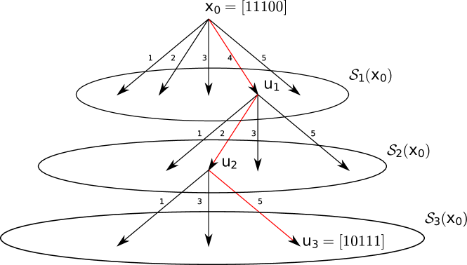
Suppose that we have a state $\mathbf{x}_{0}$ on $\mathcal{S}$. It is possible to envision taking a special type of biased self-avoiding walk (SAW) of length $k$ in the state space, in other words a sequence of states such that no state recurs in the sequence. In this type of SAW, states on sets $\{\mathcal{S}_{1}(\mathbf{x}_{0})\ldots\mathcal{S}_{k}(\mathbf{x}_{0})\}$ are visited consecutively. To generate this sequence of states $(\mathbf{u}_{1},\ldots,\mathbf{u}_{k})$, at step $i$ of the procedure a bit is chosen to be flipped from those that have not yet flipped relative to $\mathbf{x}_{0}$. Specifically, an element $\sigma_{i}$ is selected from $\mathcal{P}(\mathbf{x}_{0},\mathbf{u}_{i-1})$, with $\mathbf{u}_{0}\triangleq\mathbf{x}_{0}$, to yield state $\mathbf{u}_{i}=F(\mathbf{u}_{i-1},\sigma_{i})$, or equivalently, $\mathbf{u}_{i}=F(\mathbf{x}_{0},\sigma_{1},\ldots,\sigma_{i})$. From $\mathbf{u}_{i-1}\in\mathcal{S}_{i-1}(\mathbf{x}_{0})$, the set of states on $\mathcal{S}_{i}$ that can result from flipping a bit in $\mathcal{P}(\mathbf{x}_{0},\mathbf{u}_{i-1})$ are called the single-flip neighbours of $\mathbf{u}_{i-1}$ on $\mathcal{S}_{i}(\mathbf{x}_{0})$. The set of bits that can flip with nonzero probability are called the allowable moves at each step. A diagrammatic depiction of the SAW is shown in Figure 1.

The elements $\{\sigma_{i}\}$ are sampled in an energy-biased manner as follows:

$$f(\sigma_{i}=l|\sigma_{i-1},\ldots,\sigma_{1},\mathbf{x}_{0})=\left\{\begin{array}[]{ll}\frac{e^{-\gamma E(F(\mathbf{u}_{i-1},l))}}{\sum_{j\in\mathcal{P}(\mathbf{x}_{0},\mathbf{u}_{i-1})}e^{-\gamma E(F(\mathbf{u}_{i-1},j))}}&\begin{array}[]{ll}l\in\mathcal{P}(\mathbf{x}_{0},\mathbf{u}_{i-1})\textrm{ and }\\ \mathbf{u}_{i-1}=F(\mathbf{x}_{0},\sigma_{1},\ldots,\sigma_{i-1})\end{array}\\ \\ 0&\textrm{otherwise}\end{array}\right.$$ (3)

The larger the value that simulation parameter $\gamma$ is assigned, the more likely the proposal $f$ is to sample the lower-energy neighbors of $\mathbf{u}_{i-1}$. Conversely if it is zero, a neighbor on $\mathcal{S}_{i}(\mathbf{x}_{0})$ is selected completely at random. In principle, the value of $\gamma$ will be seen to be arbitrary; indeed it can even be different at each step of the SAW. We wil have more to say about the choice of $\gamma$, as well as the related issue of the SAW lengths, in Section 4.2.

The motivation behind using such an energy-biased scheme is that when proposing large changes of configuration, it may generate final states that are “typical” of the system’s target distribution. To make a big state-space step, one may imagine uniformly perturbing a large number of bits, but this is likely to yield states of high energy, and an MCMC algorithm will be extremely unlikely to accept the move at low temperatures.

Figure 1: A visual illustration of the move process for a SAW of length 3. The arrows represent the allowable moves from a state at that step; the red arrow shows the actual move taken in this example. With the system at state $\mathbf{x}_{0}$, the SAW begins. Bit 4 of $\mathbf{x}_{0}$ has been sampled for flipping according to Equation 3 to yield state $\mathbf{u}_{1}=[11110]$; the process is repeated until state $\mathbf{u}_{3}$ on $\mathcal{S}_{3}(\mathbf{x}_{0})$ is reached. The sequence of states taken by the SAW is $\boldsymbol{\sigma}=[4,2,5]$ .

At this point it can be seen why the term “self-avoiding” aptly describes the processes. If we imagine the state-space to be a high-dimensional lattice, with the individual states lying at the vertices and edges linking states that are single-flip neighbors, a self-avoiding walk on this graph is a sequence of states that induce a connected, acyclic subgraph of the lattice. In the move procedure we have described, a state can never occur twice at any stage within it and so the process is obviously self-avoiding.

Note however that the construction imposes a stronger condition on the state sequence; once a transition occurs from state $\mathbf{x}$ to state $F(\mathbf{x},i)$, not only may state $\mathbf{x}$ not appear again, but neither may any state $\mathbf{y}$ with $y_{i}=x_{i}$. It seems natural to ask why not to use a less constrained SAW process, namely one that avoids returns to individual states and likely more familiar to those experienced in molecular and polymer simulations, without eliminating an entire dimension at each step. In our experience, trying to construct such a SAW as a proposal requires excessive computational memory and time to yield good state-space traversal. A local minimum “basin” of a combinatoric landscape can potentially contain a massive number of states, and a process that moves by explicitly avoiding particular states may be doomed to wander within and visit a substantial portion of the basin prior to escaping.

Let $\mathbf{x}_{1}$ be the final state reached by the SAW, i.e. $\mathbf{u}_{k}$ for a length $k$ walk. By multiplying the SAW flipping probabilities, we can straightforwardly obtain the probability of moving from state $\mathbf{x}_{0}$ to $\mathbf{x}_{1}$ along the SAW $\boldsymbol{\sigma}$, which we call $f(\mathbf{x}_{1},\boldsymbol{\sigma}|\mathbf{x}_{0})$:

$$f(\mathbf{x}_{1},\boldsymbol{\sigma}|\mathbf{x}_{0})\triangleq\delta_{\mathbf{x}_{1}}[F(\mathbf{x}_{0},\boldsymbol{\sigma})]\prod_{i=1}^{k}f(\sigma_{i}|\mathbf{u}_{i-1})$$ (4)

The delta function simply enforces the fact that the final state $\mathbf{x}_{1}$ must result from the sequence of flips in $\boldsymbol{\sigma}$ from $\mathbf{x}_{0}$. The set of $\{\boldsymbol{\sigma}\}$ such that $f(\mathbf{x}_{1},\boldsymbol{\sigma}|\mathbf{x}_{0})>0$ are termed the allowable SAWs between $\mathbf{x}_{0}$ and $\mathbf{x}_{1}$.

Ideally, to implement a Metropolis-Hastings (MH) algorithm using the SAW proposal, we would like to evaluate the marginal probability of proposing $\mathbf{x}_{1}$ from $\mathbf{x}_{0}$, which we call $f(\mathbf{x}_{1}|\mathbf{x}_{0})$, so that the move would be accepted with the usual MH ratio:

$$\alpha_{m}(\mathbf{x}_{0},\mathbf{x}_{1})\triangleq\min\bigg{(}1,\frac{\pi(\mathbf{x}_{1})f(\mathbf{x}_{0}|\mathbf{x}_{1})}{\pi(\mathbf{x}_{0})f(\mathbf{x}_{1}|\mathbf{x}_{0})}\bigg{)}$$ (5)

Unfortunately, for all but small values of the walk lengths $k$, marginalization of the proposal is intractable due to the potentially massive number of allowable SAWs between the two states.

To assist in illustrating our solution to this, we recall that a sufficient condition for a Markov transition kernel $K$ to have target $\pi$ as its stationary distribution is detailed balance:

$$\pi(\mathbf{x}_{0})K(\mathbf{x}_{1}|\mathbf{x}_{0})=\pi(\mathbf{x}_{1})K(\mathbf{x}_{0}|\mathbf{x}_{1})$$ (6)

One special case obtains if we used the marginalized proposal $f(\mathbf{x}_{1}|\mathbf{x}_{0})$ followed by the MH accept rule,

$$K_{m}(\mathbf{x}_{1}|\mathbf{x}_{0})\triangleq f(\mathbf{x}_{1}|\mathbf{x}_{0})\alpha_{m}(\mathbf{x}_{0},\mathbf{x}_{1})$$ (7)

As we cannot compute $f(\mathbf{x}_{1}|\mathbf{x}_{0})$, we shall use a kernel $K(\mathbf{x}_{1},\boldsymbol{\sigma}|\mathbf{x}_{0})$ defined on the joint space of SAWs and states, and show that with some care, detailed balance (6) can still hold marginally. It will be clear, though that this does not mean that the resultant marginal kernel $K(\mathbf{x}_{1}|\mathbf{x}_{0})$ is the same as that in (7) obtained using MH acceptance on the marginal proposal .

Define the sequence reversal operator $R(\boldsymbol{\sigma})$ to simply return a sequence consisting of the elements of $\boldsymbol{\sigma}$ in reverse order; for example $R([2,3,1,4])=[4,1,3,2]$. One can straightforwardly observe that each allowable SAW $\boldsymbol{\sigma}$ from $\mathbf{x}_{0}$ to $\mathbf{x}_{1}$ can be uniquely mapped to the allowable SAW $R(\boldsymbol{\sigma})$ from $\mathbf{x}_{1}$ to $\mathbf{x}_{0}$. For example in Figure 1, the SAW $R(\boldsymbol{\sigma})=[5,2,4]$ can be seen to be allowable from $\mathbf{x}_{1}$ to $\mathbf{x}_{0}$. Next, we have the following somewhat more involved concept, a variant of which we introduced in [26]:

Definition 1.

Consider a Markov kernel $K(\mathbf{x}_{1},\boldsymbol{\sigma}|\mathbf{x}_{0})$ whose support set coincides with that of (4). We say that pathwise detailed balance holds if

$$\pi(\mathbf{x}_{0})K(\mathbf{x}_{1},\boldsymbol{\sigma}|\mathbf{x}_{0})=\pi(\mathbf{x}_{1})K(\mathbf{x}_{0},R(\boldsymbol{\sigma})|\mathbf{x}_{1})$$

for all $\boldsymbol{\sigma},\mathbf{x}_{0},\mathbf{x}_{1}$.

It turns out that pathwise detailed balance is a stronger condition than marginal detailed balance. In other words,

Proposition 1.

If the property in Definition 1 holds for a transition kernel $K$ of the type described there, then $\pi(\mathbf{x}_{0})K(\mathbf{x}_{1}|\mathbf{x}_{0})=\pi(\mathbf{x}_{1})K(\mathbf{x}_{0}|\mathbf{x}_{1})$

Proof.

Suppose, for given $\mathbf{x}_{0},\mathbf{x}_{1}$, we summed both sides of the equation enforcing pathwise detailed balance over all allowable SAWs $\{\boldsymbol{\sigma}^{\prime}\}$ from $\mathbf{x}_{0}$ to $\mathbf{x}_{1}$, i.e.

$$\sum_{\boldsymbol{\sigma}^{\prime}}\pi(\mathbf{x}_{0})K(\mathbf{x}_{1},\boldsymbol{\sigma}^{\prime}|\mathbf{x}_{0})=\sum_{\boldsymbol{\sigma}^{\prime}}\pi(\mathbf{x}_{1})K(\mathbf{x}_{0},R(\boldsymbol{\sigma}^{\prime})|\mathbf{x}_{1})$$

The left-hand summation marginalizes the kernel over allowable SAWs and hence results in $\pi(\mathbf{x}_{0})K(\mathbf{x}_{1}|\mathbf{x}_{0})$. The observation above that each allowable SAW from $\mathbf{x}_{0}$ to $\mathbf{x}_{1}$ can be reversed to yield an allowable one from $\mathbf{x}_{1}$ to $\mathbf{x}_{0}$ implies that the right-hand side is simply a re-ordered summation over all allowable SAWs from $\mathbf{x}_{1}$ to $\mathbf{x}_{0}$, and can thus be written as $\pi(\mathbf{x}_{1})K(\mathbf{x}_{0}|\mathbf{x}_{1})$. ∎

We are now ready to state the final form of the algorithm, which can be seen to instantiate a Markov chain satisfying pathwise detailed balance. After proposing $(\mathbf{x}_{1},\boldsymbol{\sigma})$ using the SAW process, we accept the move with the ratio:

$$\alpha(\mathbf{x}_{0},\mathbf{x}_{1},\boldsymbol{\sigma})\triangleq\min\bigg{(}1,\frac{\pi(\mathbf{x}_{1})f(\mathbf{x}_{0},R(\boldsymbol{\sigma})|\mathbf{x}_{1})}{\pi(\mathbf{x}_{0})f(\mathbf{x}_{1},\boldsymbol{\sigma}|\mathbf{x}_{0})}\bigg{)}$$ (8)

The computational complexity of evaluating this accept ratio is of the same order as that required to sample the proposed SAWs/state; the only additional operations required are those needed to evaluate the reverse proposal appearing in the numerator, which are completely analogous to those involved in calculating the forward proposal.

Let us take a closer look at the marginal transition kernel $K(\mathbf{x}_{1}|\mathbf{x}_{0})$. We can factor the joint proposal into:

$$f(\mathbf{x}_{1},\boldsymbol{\sigma}|\mathbf{x}_{0})=f(\mathbf{x}_{1}|\mathbf{x}_{0})f(\boldsymbol{\sigma}|\mathbf{x}_{0},\mathbf{x}_{1})$$

Of course, if we are assuming that $f(\mathbf{x}_{1}|\mathbf{x}_{0})$ is intractable to evaluate, then the conditional $f(\boldsymbol{\sigma}|\mathbf{x}_{0},\mathbf{x}_{1})$ must be so as well, but it is useful to consider. If we now summed both sides of the joint probability of moving from $\mathbf{x}_{0}$ to $\mathbf{x}_{1}$ over allowable paths, we would observe:

$$\sum_{\boldsymbol{\sigma}^{\prime}}\pi(\mathbf{x}_{0})K(\mathbf{x}_{1},\boldsymbol{\sigma}^{\prime}|\mathbf{x}_{0})=\pi(\mathbf{x}_{0})f(\mathbf{x}_{1}|\mathbf{x}_{0})\sum_{\boldsymbol{\sigma}^{\prime}}f(\boldsymbol{\sigma}^{\prime}|\mathbf{x}_{0},\mathbf{x}_{1})\alpha(\mathbf{x}_{0},\mathbf{x}_{1},\boldsymbol{\sigma}^{\prime})$$

The summation on the right-hand side is thus the conditional expectation of the accept rate given that we are attempting to move from $\mathbf{x}_{0}$ to $\mathbf{x}_{1}$; we call it

$$\alpha(\mathbf{x}_{0},\mathbf{x}_{1})\triangleq\sum_{\boldsymbol{\sigma}^{\prime}}f(\boldsymbol{\sigma}^{\prime}|\mathbf{x}_{0},\mathbf{x}_{1})\alpha(\mathbf{x}_{0},\mathbf{x}_{1},\boldsymbol{\sigma}^{\prime})$$ (9)

and it defines an effective acceptance rate between $\mathbf{x}_{0}$ and $\mathbf{x}_{1}$ under the sampling regime described since $K(\mathbf{x}_{1}|\mathbf{x}_{0})=f(\mathbf{x}_{1}|\mathbf{x}_{0})\alpha(\mathbf{x}_{0},\mathbf{x}_{1})$. It is not difficult to show that $\alpha(\mathbf{x}_{0},\mathbf{x}_{1})\neq\alpha_{m}(\mathbf{x}_{0},\mathbf{x}_{1})$, i.e. the marginal accept rate for the joint proposal is not the same as the one that results from using the marginalized proposal. In fact we can make a stronger statement:

Proposition 2.

For every pair of states $(\mathbf{x}_{0},\mathbf{x}_{1})$, $\alpha(\mathbf{x}_{0},\mathbf{x}_{1})\leq\alpha_{m}(\mathbf{x}_{0},\mathbf{x}_{1})$

Proof.

For conciseness, denote $\frac{1}{\alpha_{m}(\mathbf{x}_{0},\mathbf{x}_{1})}=\frac{\pi(\mathbf{x}_{0})f(\mathbf{x}_{1}|\mathbf{x}_{0})}{\pi(\mathbf{x}_{1})f(\mathbf{x}_{0}|\mathbf{x}_{1})}$ by $C$. Define the sets $\mathcal{A}\triangleq\{\boldsymbol{\sigma}|\frac{f(R(\boldsymbol{\sigma})|\mathbf{x}_{1},\mathbf{x}_{0})}{f(\boldsymbol{\sigma}|\mathbf{x}_{0},\mathbf{x}_{1})}\geq C\}$ and $\mathcal{\bar{A}}\triangleq\{\boldsymbol{\sigma}|\frac{f(R(\boldsymbol{\sigma})|\mathbf{x}_{1},\mathbf{x}_{0})}{f(\boldsymbol{\sigma}|\mathbf{x}_{0},\mathbf{x}_{1})}<C\}$. Then

$$\alpha(\mathbf{x}_{0},\mathbf{x}_{1}) = \sum_{\boldsymbol{\sigma}^{\prime}}f(\boldsymbol{\sigma}^{\prime}|\mathbf{x}_{0},\mathbf{x}_{1})\min\bigg{(}1,\frac{\pi(\mathbf{x}_{1})f(\mathbf{x}_{0}|\mathbf{x}_{1})f(R(\boldsymbol{\sigma}^{\prime})|\mathbf{x}_{1},\mathbf{x}_{0})}{\pi(\mathbf{x}_{0})f(\mathbf{x}_{1}|\mathbf{x}_{0})f(\boldsymbol{\sigma}^{\prime}|\mathbf{x}_{0},\mathbf{x}_{1})}\bigg{)}$$

$$= \sum_{\boldsymbol{\sigma}^{\prime}\in\mathcal{A}}f(\boldsymbol{\sigma}^{\prime}|\mathbf{x}_{0},\mathbf{x}_{1})+\frac{\pi(\mathbf{x}_{1})f(\mathbf{x}_{0}|\mathbf{x}_{1})}{\pi(\mathbf{x}_{0})f(\mathbf{x}_{1}|\mathbf{x}_{0})}\sum_{\boldsymbol{\sigma}^{\prime}\in\mathcal{\bar{A}}}f(R(\boldsymbol{\sigma}^{\prime})|\mathbf{x}_{1},\mathbf{x}_{0})$$

$$= \sum_{\boldsymbol{\sigma}^{\prime}\in\mathcal{A}}f(\boldsymbol{\sigma}^{\prime}|\mathbf{x}_{0},\mathbf{x}_{1})+\frac{1}{C}\sum_{\boldsymbol{\sigma}^{\prime}\in\mathcal{\bar{A}}}f(R(\boldsymbol{\sigma}^{\prime})|\mathbf{x}_{1},\mathbf{x}_{0})$$

But by definition, for $\boldsymbol{\sigma}\in\mathcal{A}$, $f(\boldsymbol{\sigma}|\mathbf{x}_{0},\mathbf{x}_{1})\leq\frac{1}{C}f(R(\boldsymbol{\sigma})|\mathbf{x}_{1},\mathbf{x}_{0})$.

Therefore,

$$\alpha(\mathbf{x}_{0},\mathbf{x}_{1}) \leq \frac{1}{C}\sum_{\boldsymbol{\sigma}^{\prime}\in\mathcal{A}}f(R(\boldsymbol{\sigma}^{\prime})|\mathbf{x}_{1},\mathbf{x}_{0})+\frac{1}{C}\sum_{\boldsymbol{\sigma}^{\prime}\in\mathcal{\bar{A}}}f(R(\boldsymbol{\sigma}^{\prime})|\mathbf{x}_{1},\mathbf{x}_{0})$$

$$= \frac{1}{C}\Big{(}\sum_{\boldsymbol{\sigma}^{\prime}\in\mathcal{A}}f(R(\boldsymbol{\sigma}^{\prime})|\mathbf{x}_{1},\mathbf{x}_{0})+\sum_{\boldsymbol{\sigma}^{\prime}\in\mathcal{\bar{A}}}f(R(\boldsymbol{\sigma}^{\prime})|\mathbf{x}_{1},\mathbf{x}_{0})\Big{)}$$

$$= \frac{1}{C}=\alpha_{m}(\mathbf{x}_{0},\mathbf{x}_{1})$$

∎

There is another technical consideration to address. The reader may have remarked that while detailed balance does indeed hold for our algorithm, if the SAW length is constant at $k>1$, then the resulting Markov chain is no longer irreducible. In other words, not every $\mathbf{x}\in\mathcal{S}$ is reachable with nonzero probability regardless of the initial state. For example if $k=2$ and the initial state $\mathbf{x}_{0}=[0,0,0,0,0,0]$, then the state $\mathbf{x}=[0,0,0,0,0,1]$ can never be visited. Fortunately, this is a rather easy issue to overcome; one possible strategy is to randomly choose the SAW length prior to each step from a set that ensures that the whole state space can eventually be visited. A trivial example of such a set is any collection of integers that include unity, i.e. such that single-flip moves are allowed. Another is a set that includes consecutive integers, i.e. $\{k_{0},k_{0}+1\}$ for any $k_{0}<M$. This latter choice could allow states separated by a single bit to occur in two steps; in the example above, if the set of lengths was $\{3,4\}$ then we could have $[0,0,0,0,0,0]\rightarrow[0,0,1,1,1,1]\rightarrow[0,0,0,0,0,1]$. While this shows how to enforce theoretical correctness of the algorithm, in upcoming sections we will discuss the issue of practical choice of the lengths in the set.

The experimental section discusses the practical matter of efficiently sampling the SAW for systems with sparse connectivity, such as the 2D and 3D Ising models.

3.1 Iterated SARDONICS

The SARDONICS algorithm presented in Section 3 is sufficient to work effectively on many types of system, for example Ising models with ferromagnetic interactions. This section, however, will detail a more advanced strategy for proposing states that uses the state-space SAW of Section 3 as its basic move. The overall idea is to extend the trial process so that the search for a state to propose can continue from the state resulting from a concatenated series of SAWs from $\mathbf{x}_{0}$. The reader familiar with combinatorial optimization heuristics will note the philosophical resemblance to the class of algorithms termed iterated local search [29], but will again bear in mind that in the present work, we are interested in equilibrium sampling as opposed to optimization.

We begin by noting that restriction to a single SAW is unnecessary. We can readily consider in principle an arbitrary concatenation of SAWs $(\boldsymbol{\sigma}_{1},\boldsymbol{\sigma}_{2},\ldots,\boldsymbol{\sigma}_{N})$. A straightforward extension of the SAW proposal is then to select some number of iterations $N$ (which need not be the same from one move attempt to the next,) to generate $\mathbf{x}_{1}$ from $\mathbf{x}_{0}$ by sampling from the concatenated proposal, defined to be

$$\begin{split}g(\mathbf{x}_{1},\boldsymbol{\sigma}_{1},\ldots,\boldsymbol{\sigma}_{N}|\mathbf{x}_{0})\triangleq f(\mathbf{y}^{1},\sigma_{1}|\mathbf{x}_{0})f(\mathbf{y}^{2},\sigma_{2}|\mathbf{y}^{1})\ldots\\ f(\mathbf{y}^{N},\boldsymbol{\sigma}_{N}|\mathbf{y}^{N-1})\delta_{\mathbf{x}_{1}}(\mathbf{y}^{N})\end{split}$$ (10)

and to accept the move with probability

$$\alpha(\mathbf{x}_{0},\mathbf{x}_{1},\boldsymbol{\sigma}_{1}\ldots,\boldsymbol{\sigma}_{N})=\min\bigg{(}1,\frac{\pi(\mathbf{x}_{1})g(\mathbf{x}_{0},R(\boldsymbol{\sigma}_{N}),\ldots R(\boldsymbol{\sigma}_{1})|\mathbf{x}_{1})}{\pi(\mathbf{x}_{0})g(\mathbf{x}_{1},\boldsymbol{\sigma}_{1},\ldots,\boldsymbol{\sigma}_{N}|\mathbf{x}_{0})}\bigg{)}$$ (11)

In (10), the superscripted $\{\mathbf{y}^{i}\}$ refer to the “intermediate” states on $\mathcal{S}$ generated by the flip sequences, and the functions $f$ are the SAW proposals discussed in Section 3. The proposed state $\mathbf{x}_{1}$ is identical to the final intermediate state $\mathbf{y}^{N}$; to avoid obscuring the notation with too many delta functions we take it as implicit that the the proposal evaluates to zero for intermediate states that do not follow from the flip sequences $\{\boldsymbol{\sigma}_{i}\}$.

We refer to this as the iterated SARDONICS algorithm. Its potential merit over taking a single SAW is that it may generate more distant states from $\mathbf{x}_{0}$ that are favorable. Unfortunately, a priori there is no guarantee that the final state $\mathbf{x}_{1}$ will be more worthy of acceptance than the intermediate states visited in the process; it is computationally wasteful to often propose long sequences of flips that end up rejected, especially when potentially desirable states may have been passed over. It is thus very important to choose the right value of $N$. For this reason, we will introduce Bayesian optimization techniques to adapt $N$ and other parameters automatically in the following section.

3.2 Mixture of SAWs

A further addition we made to the basic algorithm was the generalization of the proposal to a mixture of SAW processes. Each segment of the iterated procedure introduced in Section 3.1 could in principle operate at a different level of the biasing parameter $\gamma$. A possible strategy one can envision is to occasionally take a pair of SAWs with the first at a small value of $\gamma$ and the next at a large value. The first step encourages exploration away from the current state, and the second a search for a new low-energy state. More specifically, for the two SAWs $(\boldsymbol{\sigma}_{1},\boldsymbol{\sigma}_{2})$, we can have a proposal of the form:

$$f(\mathbf{x}_{1},\boldsymbol{\sigma}_{1},\boldsymbol{\sigma}_{2}|\mathbf{x}_{0})=f(\mathbf{y}^{1},\boldsymbol{\sigma}_{1}|\mathbf{x}_{0},\gamma_{L})f(\mathbf{x}_{1},\boldsymbol{\sigma}_{2}|\mathbf{y}^{1},\gamma_{H})$$

where $\gamma_{H}$ and $\gamma_{L}$ are high and low inverse temperature biases respectively. Unfortunately, such a method on its own will likely result in a high rejection rate; the numerator of the MH ratio enforcing detailed balance will be:

$$f(\mathbf{x}_{0},R(\boldsymbol{\sigma}_{2}),R(\boldsymbol{\sigma}_{1})|\mathbf{x}_{1})=f(\mathbf{y}^{1},R(\boldsymbol{\sigma}_{2})|\mathbf{x}_{1},\gamma_{L})f(\mathbf{x}_{0},R(\boldsymbol{\sigma}_{1})|\mathbf{y}^{1},\gamma_{H})$$

The probability of taking the reverse sequences will likely be very small compared to those of the forward sequences. In particular, the likelihood of descending at low-temperature biasing parameter along the sequence $R(\boldsymbol{\sigma}_{1})$, where $\boldsymbol{\sigma}_{1}$ was generated with the high-temperature parameter, will be low.

Our simple approach to dealing with this is to define the proposal to be a mixture of three types of SAW processes. The mixture weights, $P_{LL},P_{HL},P_{LH}$, with $P_{LL}+P_{LH}+P_{HL}=1$, define, respectively, the frequencies of choosing a proposal unit consisting of a pair of SAWs sampled with $(\gamma_{L},\gamma_{L})$, $(\gamma_{H},\gamma_{L})$, and $(\gamma_{L},\gamma_{H})$. The first proposal type encourages local exploration; both SAWs are biased towards low-energy states. The second one, as discussed, is desirable as it may help the sampler escape from local minima. The last one may seem somewhat strange; since it ends with sampling at $\gamma_{H}$, it will tend to generate states with high energy which will consequently be rejected. The purpose of this proposal, however, is to assist in the acceptance of the HL exploratory moves due to its presence in the mixture proposal. Thus, $P_{LH}$ is a parameter that must be carefully tuned. If it is too large, it will generate too many moves that will end up rejected due to their high energy; if too small, its potential to help the HL moves be accepted will be diminished. The mixture parameters are thus ideal candidates to explore the effectiveness of adaptive strategies to tune MCMC.

4 Adapting SARDORNICS with Bayesian Optimization

SARDONICS has several free parameters: upper and lower bounds on the SAW length ($k_{u}$ and $k_{l}$ respectively), $\gamma_{H}$, $\gamma_{L}$, $P_{LL},P_{HL},P_{LH}$ as explained in the previous section, and finally the number of concatenated SAWs $N$. We group these free parameters under the symbol $\boldsymbol{\theta}=\{k_{u},k_{l},\gamma_{H},\gamma_{L},P_{LL},P_{HL},P_{LH},N\}$. Each $\boldsymbol{\theta}$ defines a stochastic policy, where the SAW length $k$ is chosen at random in the set $[k_{l},k_{u}]$ and where the SAW processes are chosen according to the mixture probabilities $P_{LL},P_{HL},P_{LH}$. Tuning all these parameters by hand is an onerous task. Fortunately, this challenge can be surmounted using adaptation. Stochastic approximation methods, at first sight, might appear to be good candidates for carrying out this adaptation. They have become increasingly popular in the subfield of adaptive MCMC [21, 2, 51, 63]. There are a few reasons, however, that force us to consider alternatives to stochastic approximation.

In our discrete domain, there are no obvious optimal acceptance rates that could be used to construct the objective function for adaptation. Instead, we choose to optimize $\boldsymbol{\theta}$ so as to minimize the area under the auto-correlation function up to a specific lag. This objective was previously adopted in [2, 38]. One might argue that is is a reasonable objective given that researchers and practitioners often use it to diagnose the convergence of MCMC algorithms. However, the computation of gradient estimates for this objective is very involved and far from trivial [2]. This motivates the introduction of a gradient-free optimization scheme known as Bayesian optimization [43, 9]. Bayesian optimization also has the advantage that it trades-off exploration and exploitation of the objective function. In contrast, gradient methods are designed to exploit locally and may, as a result, get trapped in unsatisfactory local optima.

The proposed adaptive strategy consists of two phases: adaptation and sampling. In the adaptation phase Bayesian optimization is used to construct a randomized policy. In the sampling phase, a mixture of MCMC kernels selected according to the learned randomized policy is used to explore the target distribution. Experts in adaptive MCMC would have realized that there is no theoretical need for this two-phase procedure. Indeed, if the samplers are uniformly ergodic, which is the case in our discrete setting, and adaptation vanishes asymptotically, then ergodicity can still be established [51, 2]. However, in our setting the complexity of the adaptation scheme increases with time. Specifically, Bayesian optimization, as we shall soon outline in detail, requires fitting a Gaussian process to $I$ points, where $I$ is the number of iterations of the adaptation procedure. In the worst case, this computation is $O(I^{3})$. There are techniques based on conjugate gradients, fast multipole methods and low rank approximations to speed up this computation [15, 22]. However, none of these overcome the issue of increasing storage and computational needs. So, for pragmatic reasons, we restrict the number of adaptation steps. We will discuss the consequence of this choice in the experiments and come back to this issue in the concluding remarks.

The two phases of our adaptive strategy are discussed in more detail subsequently.

4.1 Adaptation Phase

Our objective function for adaptive MCMC is the area under the auto-correlation function up to a specific lag. This objective is intractable, but noisy observations of its value can be obtained by running the Markov chain for a few steps with a specific choice of parameters $\boldsymbol{\theta}_{i}$. Bayesian optimization can be used to propose a new candidate $\boldsymbol{\theta}_{i+1}$ by approximating the unknown function using the entire history of noisy observations and a prior over this function. The prior distribution used in this paper is a Gaussian process.

The noisy observations are used to obtain the predictive distribution of the Gaussian process. An expected utility function derived in terms of the sufficient statistics of the predictive distribution is optimized to select the next parameter value $\boldsymbol{\theta}_{i+1}$. The overall procedure is shown in Algorithm 1. We refer readers to [9] and [37] for in-depth reviews of Bayesian optimization.

1:  for $i=1,2,\dots,I$  do

2:    Run SARDONICS for $L$ steps with parameters $\boldsymbol{\theta}_{i}$.

3:    Use the drawn samples to obtain a noisy evaluation of the objective function: $z_{i}=h(\boldsymbol{\theta}_{i})+\epsilon$.

4:    Augment the observation set $\mathcal{D}_{1:i}=\{\mathcal{D}_{1:i-1},(\boldsymbol{\theta}_{i},z_{i})\}$.

5:    Update the GP’s sufficient statistics.

6:    Find $\boldsymbol{\theta}_{i+1}$ by optimizing an acquisition function: $\boldsymbol{\theta}_{i+1}=\arg\max_{\boldsymbol{\theta}}u(\boldsymbol{\theta}|\mathcal{D}_{1:i})$.

7:  end for

ALGORITHM 1 Adaptation phase of SARDONICS

The unknown objective function $h(\cdot)$ is assumed to be distributed according to a Gaussian process with mean function $m(\cdot)$ and covariance function $k(\cdot,\cdot)$:

$$h(\cdot) \sim GP(m(\cdot),k(\cdot,\cdot)).$$

We adopt a zero mean function $m(\cdot)=0$ and an anisotropic Gaussian covariance that is essentially the popular automatic relevance determination (ARD) kernel [49]:

$$k(\boldsymbol{\theta}_{j},\boldsymbol{\theta}_{k}) =\exp\left(-\frac{1}{2}(\boldsymbol{\theta}_{j}-\boldsymbol{\theta}_{k})^{T}\textrm{diag}(\psi)^{-2}(\boldsymbol{\theta}_{j}-\boldsymbol{\theta}_{k})\right)$$

where $\psi\in\mathbb{R}^{d}$ is a vector of hyper-parameters. The Gaussian process is a surrogate model for the true objective, which involves intractable expectations with respect to the invariant distribution and the MCMC transition kernels.

We assume that the noise in the measurements is Gaussian: $z_{i}=h(\boldsymbol{\theta}_{i})+\epsilon$, $\epsilon\sim\mathcal{N}(0,\sigma^{2}_{\eta})$. It is possible to adopt other noise models [11]. Our Gaussian process emulator has hyper-parameters $\psi$ and $\sigma_{\eta}$. These hyper-parameters are typically computed by maximizing the likelihood [49]. In Bayesian optimization, we can use Latin hypercube designs to select an initial set of parameters and then proceed to maximize the likelihood of the hyper-parameters iteratively [66, 55]. This is the approach followed in our experiments. However, a good alternative is to use either classical or Bayesian quadrature to integrate out the hyper-parameters [47, 53].

Let $\mathbf{z}_{1:i}\sim\mathcal{N}(0,\mathbf{K})$ be the $i$ noisy observations of the objective function obtained from previous iterations. (Note that the Markov chain is run for $L$ steps for each discrete iteration $i$. The extra index to indicate this fact has been made implicit to improve readability.) $\mathbf{z}_{1:i}$ and $h_{i+1}$ are jointly multivariate Gaussian:

$$\begin{bmatrix}\mathbf{z}_{1:i}\\ h_{i+1}\end{bmatrix} =\mathcal{N}\left(\mathbf{0},\begin{bmatrix}\mathbf{K}+\sigma^{2}_{\eta}I&\mathbf{k}^{T}\\ \mathbf{k}&k(\boldsymbol{\theta},\boldsymbol{\theta})\end{bmatrix}\right),$$

where

$$\mathbf{K} =\begin{bmatrix}k(\boldsymbol{\theta}_{1},\boldsymbol{\theta}_{1})&\ldots&k(\boldsymbol{\theta}_{1},\boldsymbol{\theta}_{i})\\ \vdots&\ddots&\vdots\\ k(\boldsymbol{\theta}_{i},\boldsymbol{\theta}_{1})&\ldots&k(\boldsymbol{\theta}_{i},\boldsymbol{\theta}_{i})\end{bmatrix}$$

and $\mathbf{k}=[k(\boldsymbol{\theta},\boldsymbol{\theta}_{1})\;\ldots\;k(\boldsymbol{\theta},\boldsymbol{\theta}_{i})]^{T}.$ All the above assumptions about the form of the prior distribution and observation model are standard and less restrictive than they might appear at first sight. The central assumption is that the objective function is smooth. For objective functions with discontinuities, we need more sophisticated surrogate functions for the cost. We refer readers to [19] and [9] for examples.

The predictive distribution for any value $\boldsymbol{\theta}$ follows from the Sherman-Morrison-Woodbury formula, where $\mathcal{D}_{1:i}=(\boldsymbol{\theta}_{1:i},\mathbf{z}_{1:i})$:

$$p(h_{i+1}|\mathcal{D}_{1:i},\boldsymbol{\theta}) =\mathcal{N}(\mu_{i}(\boldsymbol{\theta}),\sigma^{2}_{i}(\boldsymbol{\theta}))$$

$$\mu_{i}(\boldsymbol{\theta}) =\mathbf{k}^{T}(\mathbf{K+\sigma_{\eta}^{2}I})^{-1}\mathbf{z}_{1:i}$$

$$\sigma^{2}_{i}(\boldsymbol{\theta}) =k(\boldsymbol{\theta},\boldsymbol{\theta})-\mathbf{k}^{T}(\mathbf{K+\sigma_{\eta}^{2}I})^{-1}\mathbf{k}$$

The next query point $\boldsymbol{\theta}_{i+1}$ is chosen to maximize an acquisition function, $u(\boldsymbol{\theta}|\mathcal{D}_{1:i})$, that trades-off exploration (where $\sigma^{2}_{i}(\boldsymbol{\theta})$ is large) and exploitation (where $\mu_{i}(\boldsymbol{\theta})$ is high). We adopt the expected improvement over the best candidate as this acquisition function [43, 56, 9]. This is a standard acquisition function for which asymptotic rates of convergence have been proved [10]. However, we point out that there are a few other reasonable alternatives, such as Thompson sampling [41] and upper confidence bounds (UCB) on regret [59]. A comparison among these options as well as portfolio strategies to combine them appeared recently in [28]. There are several good ways of optimizing the acquisition function, including the method of DIvided RECTangles (DIRECT) of [14] and many versions of the projected Newton methods of [5]. We found DIRECT to provide a very efficient solution in our domain. Note that optimizing the acquisition function is much easier than optimizing the original objective function. This is because the acquisition functions can be easily evaluated and differentiated.

4.2 Sampling Phase

The Bayesian optimization phase results in a Gaussian process on the $I$ noisy observations of the performance criterion $\mathbf{z}_{1:I}$, taken at the corresponding locations in parameter space $\boldsymbol{\theta}_{1:I}$. This Gaussian process is used to construct a discrete stochastic policy $p(\boldsymbol{\theta}|\mathbf{z}_{1:I})$ over the parameter space $\boldsymbol{\Theta}$. The Markov chain is run with parameter settings randomly drawn from this policy at each step.

One can synthesize the policy $p(\boldsymbol{\theta}|\mathbf{z}_{1:I})$ in several ways. The simplest is to use the mean of the GP to construct a distribution proportional to $\exp(\mu(\boldsymbol{\theta}))$. This is the so-called Boltzmann policy. We can sample $M$ parameter candidates $\boldsymbol{\theta}_{i}$ according to this distribution. Our final sampler then consists of a mixture of $M$ transition kernels, where each kernel is parameterized by one of the $\boldsymbol{\theta}_{i}$, $i=1,\ldots,M$. The distribution of the samples generated in the sampling phase will approach the target distribution $\pi(\cdot)$ as the number of iterations tends to $\infty$ provided the kernels in this finite mixture are ergodic.

In high dimensions, one reasonable approach would be to use a multi-start optimizer to find maxima of the unnormalized Boltzmann policy and then perform local exploration of the modes with a simple Metropolis algorithm. This is a slight more sophisticated version of what is often referred to as the epsilon greedy policy.

The strategies discussed thus far do not take into account the uncertainty of the GP. A solution is to draw M functions according to the GP and then find he optimizer $\boldsymbol{\theta}_{i}$ of each of these functions. This is the strategy followed in [41] for the case of contextual bandits. Although this strategy works well for low dimensions, it is not clear how it can be easily scaled.

5 Experiments

Our experiments compare SARDONICS to the popular Gibbs, block-Gibbs and Swendsen-Wang samplers. Several types of binary-valued systems, all belonging to the general class of undirected graphical model called the Ising model, are used. The energy of a binary state $\mathbf{s}$, where $s_{i}\in\{-1,1\}$ is given by:

$$E(\mathbf{s})=-\sum_{(i,j)}J_{ij}s_{i}s_{j}-\sum_{i}h_{i}s_{i}$$

(One can trivially map $x_{i}\in\{0,1\}$ to $s_{i}\in\{-1,1\}$ and vice-versa.) The interaction weights $J_{ij}$ between variables $i$ and $j$ are zero if they are topologically disconnected; positive (also called “ferromagnetic”) if they tend to have the same value; and negative (“anti-ferromagnetic”) if they tend to have opposite values. The presence of interactions of mixed sign can significantly complicate Monte Carlo simulation due to the proliferation of local minimas in the energy landscape. Interaction weights of different sign produce unsatisfiable constraints and cause the system to become “frustrated”.

	Parameters of SARDONICS ($\boldsymbol{\theta}$)
	$k_{l}$	$k_{u}$	$\gamma_{L}$	$\gamma_{H}$	$P_{LL}$	$P_{HL}$	$P_{LH}$	$N$
Range	$\{1,\ldots,70\}$	$\{2,\ldots,120\}$	$[0.89,1.05]$	$[0.9,1.15]$	$[0,1]$	$[0,1]$	$[0,1]$	$\{1,\ldots,5\}$

Table 1: The ranges from which Bayesian Optimization chooses parameters for SARDONICS. The selection mechanism ensures that $k_{u}\geq k_{l}$ and $\gamma_{H}\geq\gamma_{L}$.

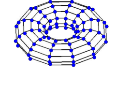
The first set of experiments considers the behavior of Gibbs, SARDONICS and Swendsen-Wang on a ferromagnetic Ising model on a planar, regular grid of size $60\times 60$. The model has connections between the nodes on one boundary to the nodes on the other boundary for each dimension. As a result of these periodic boundaries, the model is a square toroidal grid. Hence, each node has exactly four neighbors. In the first experiment, the interaction weights, $J_{ij}$, are all 1 and the biases, $h_{i}$, are all 0. We test the three algorithms on this model at three different temperatures: $1$, $2.27$ and $5$. The value $\beta=1/2.27$ corresponds to the so-called critical temperature, where many interesting phenomena arise [46] but where simulation also becomes quite difficult.

Figure 2: The 2D Ferromagnetic model with periodic (toroidal) boundaries [top left], the auto-correlations of the samplers for $T=2.27$ (critical temperature) [top right], traces of every 5 out of the $10^{5}$ samples of the energy [bottom left] and rewards obtained by the Bayesian optimization algorithm during the adaptation phase [bottom right].

The experimental protocol for this and subsequent models was the same: For 10 independent trials, run the competing samplers for a certain number of iterations, storing the sequence of energies visited. Using each trial’s energy sequence, compute the auto-correlation function (ACF). Comparison of the algorithms consisted of analyzing the energy ACF averaged over the trials. Without going into detail, a more rapidly decreasing ACF is indicative of a faster-mixing Markov chain; see for example [50]. For all the models, each sampler is run for $10^{5}$ steps. For SARDONICS, we use the first $2\times 10^{4}$ iterations to adapt its hyper-parameters. For fairness of comparison, we discard the first $2\times 10^{4}$ samples from each sampler and compute the ACF on the remaining $8\times 10^{4}$ samples. For all our experiments, we use the ranges of parameters summarized in Table I to adapt SARDONICS.

Figure 3: Auto-correlations of the samplers, on the Ferromagnetic 2D grid Ising model, for $T=1$ [top left] and $T=5$ [top right]. Traces of every 5 out of the $10^{5}$ samples of the energy at $T=1$ [bottom left] and $T=5$ [bottom right].

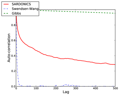
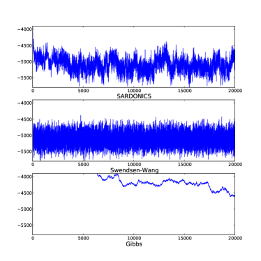
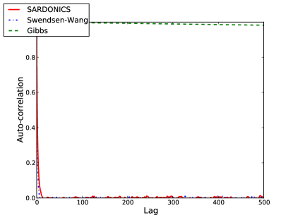
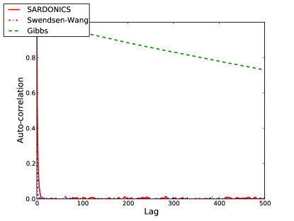
As shown in Figure 2, at the critical temperature, Swendsen-Wang does considerably better than its competitors. It is precisely for these types of lattice that Swendsen-Wang was designed to mix efficiently, through effective clustering. This part of the result is therefore not surprising. However, we must consider the performance of SARDONICS carefully. Although it does much better than Gibbs, as expected, it under-performs in comparison to Swendsen-Wang. This seems to be a consequence of the fact that the probability distribution at this temperature has many peaks. SARDONICS, despite its large moves, can get trapped in these peaks for many iterations. At temperature 5, when the distribution is flattened, the performance of SARDONICS is comparable to that of Swendsen-Wang as depicted in Figure 3. The same figure also shows the results for $T=1$, where the target distribution is even more peaked. The good performance of SARDONICS for $T=1$ might seem counterintuitive considering the previous results for $T=2.27$. An explanation is provided subsequently.

At temperatures $1$ and $2.27$, adaptation is very hard. Before the sampler converges, it is beneficial for it to take large steps to achieve lower auto-correlation. The adaptation mechanism learns this and hence automatically chooses large SAW lengths. But after the sampler converges, large steps can take the sampler out of the high-probability region thus leading to low acceptance. If the sampler hits the peak during adaptation then it learns to choose small SAW lengths. This may also be problematic if we restart the sampler from a different state. This points out one of the dangers of having finite adaptation schemes. A simple solution, in this particular case, is to change the bounds on the SAW lengths manually. This enables SARDONICS to achieve performance comparable to that of Swendsen Wang for these nearly deterministic models, as shown in Figure 3 for $T=1$. However, ideally, infinite adaptation mechanisms might provide a more principled and general solution.

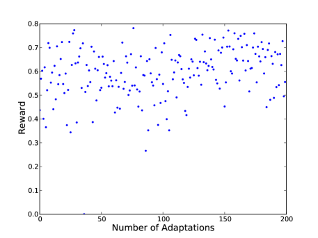
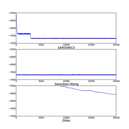
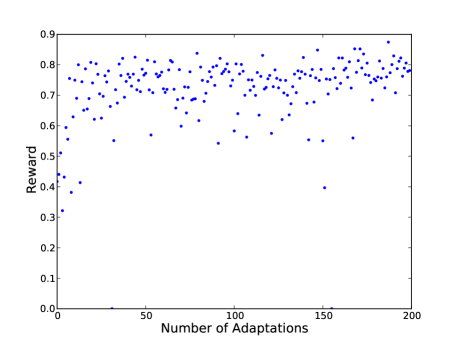
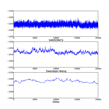
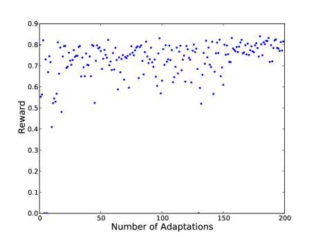
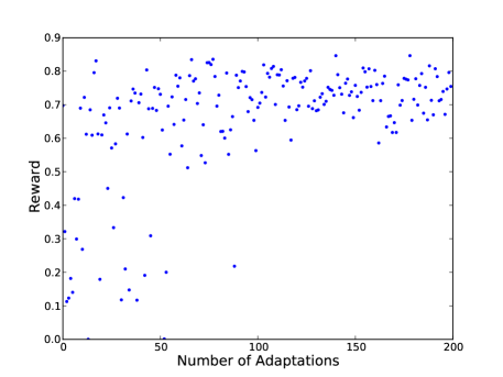
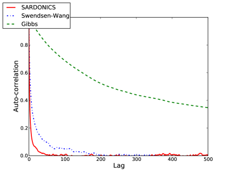
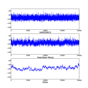
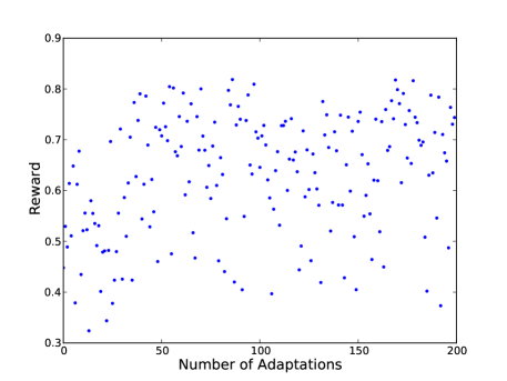
In addition to studying the effect of temperature changes on the performance of the algorithms, we also investigate their sensitivity with respect to the addition of unsatisfiable constraints. To accomplish this, we set the interaction weights $J_{ij}$ and the biases $h_{i}$ uniformly at random on the set $\{-1,1\}$. We set the temperature to $T=1.0$. We refer to this model as the frustrated 2D grid Ising model. As shown by the auto-correlations and energy traces plotted in Figure 4, SARDONICS does considerably better than its rivals. It is interesting to note that Swendsen-Wang does much worse on this model as the unsatisfiable constraints hinder effective clustering. The figure also shows the reward obtained by the Bayesian optimization scheme as a function of the number of adaptations. The adaptation algorithm traded-off exploration and exploitation effectively in this case.

Figure 4: Frustrated 2D grid Ising model with periodic boundaries [top left], auto-correlations of the three samplers [top right], traces of the last 20000 of 100000 samples of the energy [bottom left] and rewards obtained by the Bayesian optimization algorithm during the adaptation phase [bottom right].

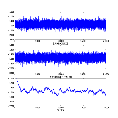
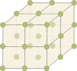
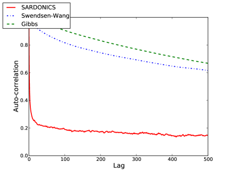
The third batch of experiments compares the algorithms on an Ising model where the variables are topologically structured as a $9\times 9\times 9$ three-dimensional cube, $J_{ij}$ are uniformly sampled from the set $\{-1,1\}$, and the $h_{i}$ are zero. $\beta$ was set to $1.0$, corresponding to a lower temperature than the value of $0.9$, at which it is known [39] that, roughly speaking, regions of the state space become very difficult to visit from one another via traditional Monte Carlo simulation. Figure 5 shows that for this more densely connected model, the performance of Swendsen-Wang deteriorates substantially. However, SARDONICS still mixes reasonably well.

Figure 5: Frustrated 3D cube Ising model with periodic boundaries (for visualization simplicity, the boundary edges are not shown) [top left], auto-correlations of the three samplers [top right], traces of the last 20000 of 100000 samples of the energy [bottom left] and rewards obtained by the Bayesian optimization algorithm during the adaptation phase [bottom right].

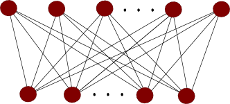
While the three-dimensional-cube spin-glass is a much harder problem than the 2D ferromagnet, it represents a worst case scenario. One would hope that problems arising in practice will have structure in the potentials that would ease the problem of inference. For this reason, the third experimental set consisted of runs on a restricted Boltzmann machine [58] with parameters trained from natural image patches via stochastic maximum likelihood [61, 40]. RBMs are bipartite undirected probabilistic graphical models. The variables on one side are often referred to as “visible units”, while the others are called “hidden units”. Each visible unit is connected to all hidden units. However there are no connections among the hidden units and among the visible units. Therefore, given the visible units, the hidden units are conditionally independent and vice-versa. Our model consisted of 784 visible and 500 hidden units. The model is illustrated in Figure 6.

Figure 6: Frustrated 3D cube Ising model with periodic boundaries [top left], auto-correlations of the three samplers [top right], traces of the last 20000 of 100000 samples of the energy [bottom left] and rewards obtained by the Bayesian optimization algorithm during the adaptation phase [bottom right].

Figure 7: Trace of the last 20000 of 100000 samples of the energy for the Swendsen-Wang sampler. As we can see, the sampler performs poorly on the RBM model.

Figure 8: RBM parameters. Each image corresponds to the parameters connecting a specific hidden unit to the entire set of visible units.

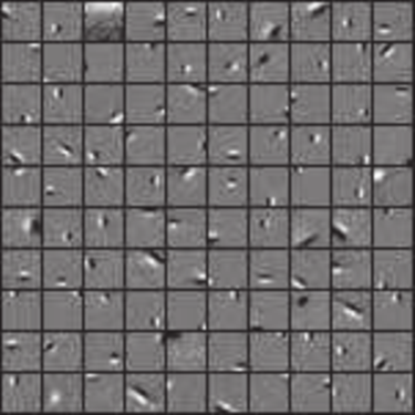
The pre-learned interaction parameters capture local regularities of natural images [31]. Some of these parameters are depicted as images in Figure 8. The parameter $\beta$ was set to one. The total number of variables and edges in the graph were thus 1284 and 392000 respectively.

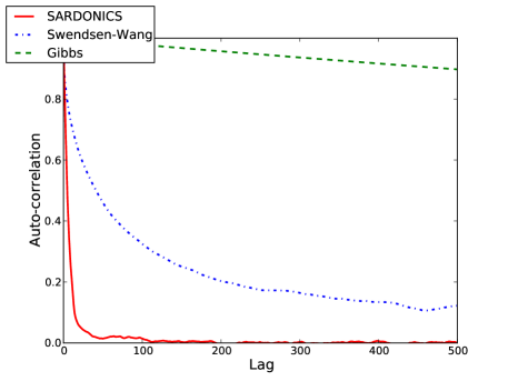
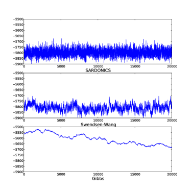
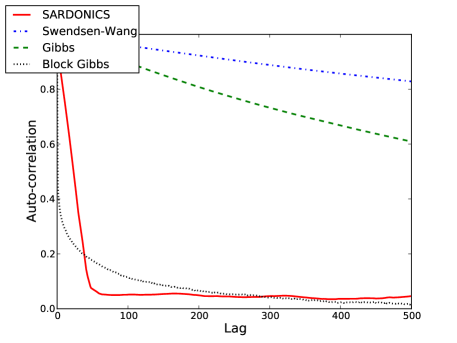
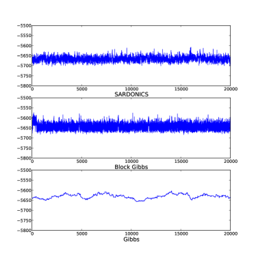
Figures 6 and 7 show the results. Again SARDONICS mixes significantly better than Swendsen-Wang and the naive Gibbs sampler. Swendsen-Wang performs poorly on this model. As shown in Figure 7, it mixes slowly and fails to converge after $10^{5}$ iterations.

For this bipartite model, it is possible to carry out block-Gibbs sampling (the standard method of choice). Encouragingly, SARDONICS compares well against this popular block strategy. This is important, because computational neuro-scientists would like to add lateral connections among the hidden units, in which case block-Gibbs would no longer apply unless the connections form a tree structure. SARDONICS thus promises to empower computational neuro-scientists to address more sophisticated models of perception. The catch is that at present SARDONICS takes considerably more time than block-Gibbs sampling for these models. We discuss this issue in greater length in the following section.

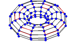
Finally, we consider a frustrated 128-bit chimera lattice that arises in the construction of quantum computers [7]. As depicted in Figure 9, SARDONICS once again outperforms its competitors.

Figure 9: Chimera lattice [top left], auto-correlations of the three samplers [top right], traces of the last 20000 of 100000 samples of the energy [bottom left] and rewards obtained by the Bayesian optimization algorithm during the adaptation phase [bottom right].

5.1 Computational considerations

	Samplers
Models	SARDONICS	Swendsen-Wang	Gibbs	Block Gibbs
Ferromagnetic Ising Model	20 minutes	50 minutes	tens of seconds	N/A
Frustrated 2D Ising Model	20 minutes	50 minutes	tens of seconds	N/A
Frustrated 3D Ising Model	10 minutes	a few minutes	tens of seconds	N/A
RBM	10 hours	a few hours	20 minutes	a few minutes
Chimera	a few minutes	tens of seconds	tens of seconds	N/A

Table 2: Rough computation time for each sampler on different models. All samplers are run on the same computer with 8 CPUs. The Swendsen-Wang sampler is coded in Matlab with the computationally intensive part written in C. The SARDONICS sampler is coded in Python also with its computationally intensive part coded in C. The Gibbs and block Gibbs samplers are coded in Python. The Swendsen-Wang and block Gibbs samplers take advantage of parallelism via parallel numerical linear algebra operations. The SARDONICS sampler and the Gibbs sampler, however, run on a single CPU. The adaptation time of SARDONICS is also included.

The bulk of the computational time of the SARDONICS algorithm is spent in generating states with the SAW proposal. At each step of the process, a component from a discrete probability vector, corresponding to the variable to flip, must be sampled. Naively, the time needed to do so scales linearly with the length $l$ of the vector. In graphical models of sparse connectivity, however, it is possible achieve a dramatic computational speedup by storing the vector in a binary heap. Sampling from a heap is of $O(\log l)$, but for sparsely connected models, updating the heap in response to a flip, which entails replacing the energy changes that would result if the flipped variable’s neighboring variables were themselves to flip, is also of logarithmic complexity. In contrast, for a densely connected model, the heap update would be of $O(M\log l)$ where $M$ is the maximum degree of the graph, while recomputing the probability vector in the naive method is $O(M)$. The simple method is thus cheaper for dense models. In our experiments, we implemented SARDONICS with the binary heap despite the fact that the RBM is a densely connected model.

For densely connected models, one could easily parallelize the computation of generating states with the SAW proposal. Suppose we have $n$ parallel processes. Each process $P$ holds one section $U_{p}$ of the unnormalized probability vector $U$. To sample from the discrete vector in parallel, each parallel process can sample one variable $v_{p}$ to flip according to $U_{p}$. Each process also calculates the sum of its section of the unnormalized probability vector $s_{p}$. Then the variable to flip is sampled from the set $\{v_{p}:1\leq p\leq n\}$ proportional to the discrete probability vector $[s_{1},s_{2},...,s_{n}]$. To update $U$ in response to a flip, we could use the naive method mentioned above. If we divide the $U$ evenly among processes and assume equal processor speed, sampling from and updating the unnormalized probability vector would take $O(\frac{M+l}{n}+n)$ operations. When $n$ is small compared to $M+l$, we could achieve near linear speed up.

We compare, in table II, the amount of time it takes to draw $10^{5}$ samples using different samplers. In principle, it is unwise to compare the computational time of samplers when this comparison depends on specific implementation details and architecture. The table simply provides rough estimates. The astute reader might be thinking that we could run Gibbs for the same time as SARDONICS and expect similar performance. This is however not what happens. We tested this hypothesis and found Gibbs to still underperform. Moreover, in some cases, Gibbs can get trapped as a result of being a small move sampler.

The computational complexity of SARDONICS is affected by the degree of the graph, whereas the complexity of Swendsen-Wang increases with the number of edges in the graph. So for large sparsely-connected graphs, we expect SARDONICS to have a competing edge over Swendsen-Wang, as already demonstrated to some extent in the experiments.

6 Discussion

The results indicate that the proposed sampler mixes very well in a broad range of models. However, as already pointed out, we believe that we need to consider alternatives to nonparametric methods in Bayesian optimization. Parametric methods would enable us to carry out infinite adaptation. This should solve the problems pointed out in the discussion of the results on the ferromagnetic 2D Ising model. Another important avenue of future work is to develop a multi-core implementation of SARDONICS as outlined in the previous section.

References

- [1] D. H. Ackley, G. Hinton, and T.. Sejnowski. A learning algorithm for Boltzmann machines. Cognitive Science, 9:147–169, 1985.
- [2] Christophe Andrieu and Christian Robert. Controlled MCMC for optimal sampling. Technical Report 0125, Cahiers de Mathematiques du Ceremade, Universite Paris-Dauphine, 2001.
- [3] F Barahona. On the computational complexity of Ising spin glass models. Journal of Physics A: Mathematical and General, 15(10):3241, 1982.
- [4] Bernd A. Berg and Thomas Neuhaus. Multicanonical algorithms for first order phase transitions. Physics Letters B, 267(2):249 – 253, 1991.
- [5] Dimitri P. Bertsekas. Projected Newton methods for optimization problems with simple constraints. SIAM Journal on Control and Optimization, 20(2):221–246, 1982.
- [6] Julian Besag. Spatial interaction and the statistical analysis of lattice systems. J. Roy. Statist. Soc., Ser. B, 36:192–236, 1974.
- [7] Zhengbing Bian, Fabian Chudak, William G. Macready, and Geordie Rose. The Ising model: teaching an old problem new tricks. Technical report, D-Wave Systems, 2011.
- [8] David M. Blei, Andrew Y. Ng, and Michael I. Jordan. Latent Dirichlet allocation. J. Mach. Learn. Res., 3:993–1022, 2003.
- [9] Eric Brochu, Vlad M Cora, and Nando de Freitas. A tutorial on Bayesian optimization of expensive cost functions. Technical Report TR-2009-023, University of British Columbia, Department of Computer Science, 2009.
- [10] Adam D Bull. Convergence rates of efficient global optimization algorithms. Technical Report arXiv:1101.3501v2, 2011.
- [11] P. J. Diggle, J. A. Tawn, and R. A. Moyeed. Model-based geostatistics. Journal of the Royal Statistical Society. Series C (Applied Statistics), 47(3):299–350, 1998.
- [12] S Duane, A D Kennedy, B J Pendleton, and D Roweth. Hybrid Monte Carlo. Physics Letters B, 195(2):216–222, 1987.
- [13] David J. Earl and Michael W. Deem. Parallel tempering: Theory, applications, and new perspectives. Phys. Chem. Chem. Phys., 7:3910–3916, 2005.
- [14] Daniel E Finkel. DIRECT Optimization Algorithm User Guide. Center for Research in Scientific Computation, North Carolina State University, 2003.
- [15] Nando De Freitas, Yang Wang, Maryam Mahdaviani, and Dustin Lang. Fast Krylov methods for N-body learning. In Y. Weiss, B. Schölkopf, and J. Platt, editors, Advances in Neural Information Processing Systems, pages 251–258. MIT Press, 2005.
- [16] Charles J Geyer. Markov Chain Monte Carlo maximum likelihood. In Computer Science and Statistics: 23rd Symposium on the Interface, pages 156–163, 1991.
- [17] Mark Girolami and Ben Calderhead. Riemann manifold Langevin and Hamiltonian Monte Carlo methods. Journal of the Royal Statistical Society: Series B (Statistical Methodology), 73(2):123–214, 2011.
- [18] F. Glover. Tabu search – Part I. ORSA Journal on Computing, 1:190–206, 1989.
- [19] Robert B Gramacy, Herbert K. H. Lee, and William MacReady. Parameter space exploration with gaussian process trees. In Proceedings of the International Conference on Machine Learning, pages 353–360. Omnipress and ACM Digital Library, 2004.
- [20] J. Gubernatis and N. Hatano. The multicanonical monte carlo method. Computing in Science Engineering, 2(2):95–102, 2000.
- [21] Heikki Haario, Eero Saksman, and Johanna Tamminen. An adaptive Metropolis algorithm. Bernoulli, 7(2):223–242, 2001.
- [22] N. Halko, P. G. Martinsson, , and J. A. Tropp. Finding structure with randomness: Probabilistic algorithms for constructing approximate matrix decompositions. Science, 53(2):217–288, 2011.
- [23] Firas Hamze and Nando de Freitas. From fields to trees. In Uncertainty in Artificial Intelligence, pages 243–250, 2004.
- [24] Firas Hamze and Nando de Freitas. Hot Coupling: a particle approach to inference and normalization on pairwise undirected graphs. Advances in Neural Information Processing Systems, 18:491–498, 2005.
- [25] Firas Hamze and Nando de Freitas. Large-flip importance sampling. In Uncertainty in Artificial Intelligence, pages 167–174, 2007.
- [26] Firas Hamze and Nando de Freitas. Intracluster moves for constrained discrete-space MCMC. In Uncertainty in Artificial Intelligence, pages 236–243, 2010.
- [27] Geoffrey Hinton and Ruslan Salakhutdinov. Reducing the dimensionality of data with neural networks. Science, 313(5786):504–507, 2006.
- [28] Matthew Hoffman, Eric Brochu, and Nando de Freitas. Portfolio allocation for Bayesian optimization. In Uncertainty in Artificial Intelligence, pages 327–336, 2011.
- [29] Holger H. Hoos and Thomas Stutzle. Stochastic Local Search: Foundations and Applications. Elsevier, Morgan Kaufmann, 2004.
- [30] J J Hopfield. Neurons with graded response have collective computational properties like those of two-state neurons. Proceedings of the National Academy of Sciences, 81(10):3088–3092, 1984.
- [31] A. Hyvarinen, J. Hurri, and P.O. Hoyer. Natural Image Statistics.
- [32] Ross Kindermann and J. Laurie Snell. Markov Random Fields and their Applications. Amer. Math. Soc., 1980.
- [33] Hendrik Kück and Nando de Freitas. Learning about individuals from group statistics. In Uncertainty in Artificial Intelligence, pages 332–339, 2005.
- [34] Honglak Lee, Roger Grosse, Rajesh Ranganath, and Andrew Y. Ng. Convolutional deep belief networks for scalable unsupervised learning of hierarchical representations. In International Conference on Machine Learning, pages 609–616, 2009.
- [35] Jun S. Liu. Monte Carlo strategies in scientific computing. Springer, 2001.
- [36] Jun S. Liu, Junni L. Zhang, Michael J. Palumbo, and Charles E. Lawrence. Bayesian clustering with variable and transformation selections. Bayesian Statistics, 7:249–275, 2003.
- [37] Daniel Lizotte. Practical Bayesian Optimization. PhD thesis, University of Alberta, Edmonton, Alberta, Canada, 2008.
- [38] Nimalan Mahendran, Ziyu Wang, Firas Hamze, and Nando de Freitas. Bayesian optimization for adaptive MCMC. Technical Report arXiv:1110.6497v1, 2011.
- [39] E. Marinari, G. Parisi, and JJ Ruiz-Lorenzo. Numerical simulations of spin glass systems. Spin Glasses and Random Fields, pages 59–98, 1997.
- [40] Benjamin Marlin, Kevin Swersky, Bo Chen, and Nando de Freitas. Inductive principles for restricted Boltzmann machine learning. In Artificial Intelligence and Statistics, pages 509–516, 2010.
- [41] Benedict C May, Nathan Korda, Anthony Lee, and David S Leslie. Optimistic Bayesian sampling in contextual bandit problems. 2011.
- [42] Roland Memisevic and Geoffrey Hinton. Learning to represent spatial transformations with factored higher-order Boltzmann machines. Neural Computation, 22:1473–1492, 2009.
- [43] Jonas Močkus. The Bayesian approach to global optimization. In System Modeling and Optimization, volume 38, pages 473–481. Springer Berlin / Heidelberg, 1982.
- [44] J. D. Munoz, M. A. Novotny, and S. J. Mitchell. Rejection-free Monte Carlo algorithms for models with continuous degrees of freedom. Phys. Rev. E, 67, 2003.
- [45] Radford M Neal. MCMC using Hamiltonian dynamics. Handbook of Markov Chain Monte Carlo, 54:113–162, 2010.
- [46] M. Newman and G. Barkema. Monte Carlo Methods in Statistical Physics. Oxford University Press, 1999.
- [47] M.A. Osborne, R. Garnett, and S. Roberts. Active data selection for sensor networks with faults and changepoints. In IEEE International Conference on Advanced Information Networking and Applications, 2010.
- [48] Marc’Aurelio Ranzato, Volodymyr Mnih, and Geoffrey Hinton. How to generate realistic images using gated MRF’s. In Advances in Neural Information Processing Systems, pages 2002–2010, 2010.
- [49] Carl Edward Rasmussen and Christopher K I Williams. Gaussian Processes for Machine Learning. MIT Press, Cambridge, Massachusetts, 2006.
- [50] Christian P. Robert and George Casella. Monte Carlo Statistical Methods. Springer, 2nd edition, 2004.
- [51] Gareth O. Roberts and Jeffrey S. Rosenthal. Examples of adaptive MCMC. Journal of Computational and Graphical Statistics, 18(2):349–367, June 2009.
- [52] Marshall N. Rosenbluth and Arianna W. Rosenbluth. Monte Carlo calculation of the average extension of molecular chains. J. Chem. Phys., 23:356–359, 1955.
- [53] Havard Rue, Sara Martino, and Nicolas Chopin. Approximate Bayesian inference for latent Gaussian models by using integrated nested Laplace approximations. Journal Of The Royal Statistical Society Series B, 71(2):319–392, 2009.
- [54] Ruslan Salakhutdinov and Iain Murray. On the quantitative analysis of Deep Belief Networks. In International Conference on Machine Learning, pages 872–879, 2008.
- [55] T J Santner, B Williams, and W Notz. The Design and Analysis of Computer Experiments. Springer, 2003.
- [56] Matthias Schonlau, William J. Welch, and Donald R. Jones. Global versus local search in constrained optimization of computer models. Lecture Notes-Monograph Series, 34:11–25, 1998.
- [57] Jörn I. Siepmann and Daan Frenkel. Configurational bias Monte Carlo: a new sampling scheme for flexible chains. Molecular Physics: An International Journal at the Interface Between Chemistry and Physics, 75(1):59–70, 1992.
- [58] P. Smolensky. Information processing in dynamical systems: Foundations of harmony theory. Parallel distributed processing: Explorations in the microstructure of cognition, vol. 1: foundations, pages 194–281, 1986.
- [59] Niranjan Srinivas, Andreas Krause, Sham M Kakade, and Matthias Seeger. Gaussian process optimization in the bandit setting: No regret and experimental design. In International Conference on Machine Learning, 2010.
- [60] Robert H. Swendsen and Jian-Sheng Wang. Nonuniversal critical dynamics in Monte Carlo simulations. Phys. Rev. Lett., 58(2):86–88, 1987.
- [61] Kevin Swersky, Bo Chen, Ben Marlin, and Nando de Freitas. A tutorial on stochastic approximation algorithms for training restricted Boltzmann machines and deep belief nets. In Information Theory and Applications Workshop, pages 1 –10, 2010.
- [62] S. S. Tham, A. Doucet, and R. Kotagiri. Sparse Bayesian learning for regression and classification using Markov chain Monte Carlo. In International Conference on Machine Learning, pages 634–641, 2002.
- [63] Matti Vihola. Grapham: Graphical models with adaptive random walk Metropolis algorithms. Computational Statistics and Data Analysis, 54(1):49 – 54, 2010.
- [64] Fugao Wang and D. P. Landau. Efficient, multiple-range random walk algorithm to calculate the density of states. Phys. Rev. Lett., 86:2050–2053, 2001.
- [65] Dominic J. A. Welsh. Complexity: knots, colourings and counting. Cambridge University Press, 1993.
- [66] Kenny Q. Ye. Orthogonal column Latin hypercubes and their application in computer experiments. Journal of the American Statistical Association, 93(444):1430–1439, 1998.