Density classification on infinite
lattices and trees
Abstract
Consider an infinite graph with nodes initially labeled by independent Bernoulli random variables of parameter . We address the density classification problem, that is, we want to design a (probabilistic or deterministic) cellular automaton or a finite-range interacting particle system that evolves on this graph and decides whether is smaller or larger than . Precisely, the trajectories should converge to the uniform configuration with only if , and only if . We present solutions to that problem on , for any , and on the regular infinite trees. For , we propose some candidates that we back up with numerical simulations.
Keywords. Cellular automata, interacting particle systems, density classification, percolation.
1 Introduction
Consider a finite or a countably infinite set of cells, which are spatially arranged according to a group structure . We are interested in the density classification problem, which consists of deciding in a decentralised way, if an initial configuration on contains more 0’s or more 1’s. More precisely, the goal is to design a deterministic or probabilistic dynamical system that evolves in the configuration space with a local and homogeneous updating rule and whose trajectories converge to or to if the initial configuration contains more 0’s or more 1’s, respectively. To attack the problem, two natural instantiations of dynamical systems are considered, one with synchronous updates of the cells, and one with asynchronous updates. In the first case, time is discrete, all cells are updated at each time step, and the model is known as a Probabilistic Cellular Automaton (PCA) [3]. A Cellular Automaton (CA) is a PCA in which the updating rule is deterministic. In the second case, time is continuous, cells are updated at random instants, at most one cell is updated at any given time, and the model is known as a (finite range) Interacting Particle System (IPS) [16].
The general spirit of the problem is that of distributed computing: gathering a global information by exchanging only local information. The challenge is two-fold: first, it is impossible to centralise the information (cells are indistinguishable); second, it is impossible to use classical counting techniques (cells contain only a binary information).
The density classification problem was originally introduced for rings of finite size () and for synchronous models [17]. After experimentally observing that finding good rules to perform this task was difficult, it was shown that perfect classification with CA is impossible, that is, there exists no given CA that solves the density classification problem for all values of [14]. This result however did not stop the quest for the best – although imperfect – models as nothing was known about how well CA could perform. The use of PCA opened a new path [6, 18] and it was shown that there exist PCA that can solve the problem with an arbitrary precision [4]. In the present paper, Prop. 1, we complement the results from [14, 4] by showing that there exists no PCA that solves the density classification problem for all values of .
The challenge is now to extend the research to infinite groups (whose Cayley graphs are lattices or regular trees). First, we need to specify the meaning of “having more 0’s or more 1’s” in this context. Consider a random configuration on obtained by assigning independently to each cell a value 1 with probability and a value 0 with probability . We say that a model “classifies the density” if the trajectories converge weakly to for , and to for . A couple of conjectures and negative results exist in the literature. Density classification on is considered in [2] under the name of “bifurcation”. The authors study variants of the famous voter model IPS [16, Ch. V] and they propose two instances that are conjectured to bifurcate. The density classification question has also been addressed for the Glauber dynamic associated to the Ising model at temperature 0, both for lattices and for trees [5, 11, 12]. The Glauber dynamic defines an IPS or PCA having and as invariant measures. Depending on the cases, there is either a proof that the Glauber dynamic does not classify the density, or a conjecture that it does with a proof only for densities sufficiently close to or .
The density classification problem has been approached with different perspectives on finite and infinite groups, as emphasised by the results collected above. For finite groups, the problem is studied per se, as a benchmark for understanding the power and limitations of PCA as a computational model. The community involved is rather on the computer science side. For infinite groups, the goal is to understand the dynamics of specific models that are relevant in statistical mechanics. The community involved is rather on the theoretical physics and probability theory side.
The aim of the present paper is to investigate how to generalise the finite group approach to the infinite group case. We want to build models of PCA and IPS, as simple as possible, that correct random noise in the initial configuration, even if the density of errors is close to . We consider the groups , whose Cayley graphs are lattices (Section 3), and the free groups, whose Cayley graphs are infinite regular trees (Section 4). In all cases, except for , we obtain both PCA and IPS models that classify the density. To the best of our knowledge, they constitute the first known such examples. The case of is more complicated and could be linked to the so-called positive rates conjecture [8]. We provide some potential candidates for density classification together with simulation experiments (Section 5).
2 Defining the density classification problem
Let be a finite or countable set of cells equipped with a group structure. Set , the alphabet, and , the set of configurations. For and , denote by the number of occurences of in .
2.1 PCA and IPS
Given a finite set , a transition function of neighbourhood is a function . The cellular automaton (CA) of transition function is the application defined by:
When the group is or , we denote as usual the law of by the sign , so that the definition can be written:
Probabilistic cellular automata (PCA) are an extension of classical CA: the transition function is now a function , where denotes the set of probability measures on . At each time step, the cells are updated synchronously and independently, according to a distribution depending on a finite neighbourhood [3]. This defines an application . The image of a measure is denoted by .
The analog of PCA in continuous time are (finite-range) interacting particle systems (IPS) [16]. IPS are characterised by a finite neighbourhood , and a transition function (or ). We attach random and independent clocks to the cells of . For a given cell, the instants of at which the clock rings form a Poisson process of parameter 1. Let be the configuration at time of the process. If the clock at cell rings at instant , the state of the cell is updated into (or according to the probability measure ). This defines a transition semigroup , with . If the initial measure is , the distribution of the process at time is given by .
In a PCA, all cells are updated at each time step, in a “synchronous” way. On the other hand, for an IPS, the updating is “asynchronous”. Indeed, the probability of having two clocks ringing at the same instant is 0.
Observe that PCA are discrete-time Markov chains, while IPS are continuous-time Markov processes. A measure is said to be an invariant mesasure of a process , resp. , if , resp. for all .
2.2 The density classification problem on
The density classification problem was originally stated as follows: find a finite neighbourhood and a transition function such that for any integer and any configuration , when applying the CA of transition function to , the sequence of iterates reaches the fixed point if and the fixed point if . Land and Belew [14] have proved that there exists no CA that perfectly performs this density classification task for all values of . We now prove that this negative result can be extended to the PCA. It provides at the same time a new proof for CA as a particular case.
Denote by the probability measure that corresponds to a Dirac distribution centred on .
Proposition 1.
There exists no PCA or IPS that solves perfectly the density classification problem on , that is, for any integer , and for any configuration , converges to if and to if .
Proof.
We carry out the proof for PCA. For IPS, the argument is similar and even simpler. Let us assume that is a PCA that solves perfectly the density classification problem on . Let be the neighbourhood of , and let be such that . We will prove that for any (with ), the number of occurrences of after application of to is almost surely equal to . Let us assume that it is not the case. Then, we have:
| (1) |
Assume for instance that (the case is treated similarly). We first assume that . For some integers , let us consider the configuration . We have . Let be the suffix of length of , and let be the prefix of length of . By applying (1), it follows that:
Set . We have . For big enough, if we set to be the largest integer such that , we have:
So, with a positive probability, we can reach a configuration with more ones than zeros starting from a configuration with more zeros than ones. Since classifies the density with probability , the new configuration can be considered as an initial condition that needs to be classified and will thus almost surely evolve to the fixed point , that is, a bad classification will occur, which contradicts our hypothesis.
The case is analogous, except that we now consider configurations of the form and choose the integers such that and .
We have proved that for any (with ), the number of occurrences of ones after application of to is almost surely equal to . This is in contradiction with the fact that classifies the density. ∎
This proposition can be extended to larger dimensions: for any , there is no PCA or IPS that classifies perfectly the density on all the groups of the form .
2.3 The density classification problem on infinite groups
Let us define formally the density classification problem on infinite groups.
We denote by the Bernoulli measure of parameter , that is, the product measure of density on . A realisation of is obtained by assigning independently to each element of a label with probability and a label with probability . We denote respectively by and the two uniform configurations and and by the probability measure that corresponds to a Dirac distribution centred on .
The density classification problem is to find a PCA or an IPS , such that:
| (2) |
The notation stands for the weak convergence of measures. In our case, the interpretation is that for any finite subset , the probability that at time , all the cells of are labelled by (resp. by ) tends to if (resp. if ). Or equivalently, that for any single cell, the probability that it is labelled by (resp. by ) tends to if (resp. if ).
2.4 From subgroups to groups
Next proposition has the following consequence: given a process that classifies the density on , we can design a new one that classifies on for . The idea is to divide into -layers and to apply the original process independently on each layer.
Proposition 2.
Let be a subgroup of , and let be a process (PCA or IPS) of neighbourhood and transition function that classifies the density on . We denote by the process on having the same neighbourhood and the same transition function . Then, classifies the density on .
Proof.
Since is a subgroup, the group is partitioned into a union of classes We have , so that if an element is in some class , then for any , the element is also in . Since classifies the density, on each class , the process satisfies (2). Thus for any cell of , the probability that it is labelled by (resp. by ) tends to if (resp. if ). ∎
3 Classifying the density on : Toom’s rule
To classify the density on , a natural idea is to apply the majority rule on a cell and its four direct neighbours. Unfortunately, this does not work, neither in the CA nor in the IPS version. Indeed, an elementary square of four cells in state 1 on a background of 0’s is a fixed point for the process. For , monochromatic elementary squares of both colors appear almost surely in the initial configuration which makes the convergence to or impossible.
Another idea is to apply the majority rule on the four nearest neighbours (excluding the cell itself) and to choose uniformly the new state of the cell in case of equality. In the IPS setting, this process is known as the Glauber dynamics associated to the Ising model. It has been conjectured to classify the density, but the result has been proved only for values of that are sufficiently close to or [5].
To overcome the difficulty, we consider the majority CA but on the asymmetric neighbourhood . We prove that this CA, known as Toom’s rule [3, 7], classifies the density on . Our proof relies on the properties of the percolation clusters on the triangular lattice [10]. We then define an IPS inspired by this local rule and prove with the same techniques that it also classifies the density.
3.1 A cellular automaton that classifies the density
Let us denote by , the majority function, so that and
Theorem 1.
The cellular automaton defined by:
for any classifies the density.
Proof.
By symmetry, it is sufficient to prove that if , then converges weakly to .
Let us consider the triangular lattice of sites (vertices) and bonds (edges) . We recall that a -cluster is a subset of connected sites labelled by which is maximal for inclusion. The site percolation threshold on the triangular lattice is equal to so that, for , there exists almost surely no infinite -cluster [10]. Thus, if denotes the set of sites labelled by , the set consists almost surely of a countable union of finite -clusters. Moreover, the size of the -clusters decays exponentially: there exist some constants and such that the probability for a given site to be part of a -cluster of size larger than is smaller than , see [10].
Let us describe how the -clusters are transformed by the action of the CA. For , let be the configuration defined by if and otherwise. Let be the subset of such that . By a simple symmetry argument, this last equality is equivalent to . We observe the following.
-
•
The rule does not break up or connect different -clusters (proved by Gács [7, Fact 3.1]). More precisely, if consists of the -clusters , then the components of are the nonempty sets among .
-
•
Any finite -cluster disappears in finite time: if is a finite and connected subset of , then there exists an integer such that . This is the eroder property [3].
-
•
Let us consider a -cluster and a rectangle in which it is contained. Then the -cluster always remains within this rectangle. More precisely, if is a rectangle set, that is, a set of the form , and if , then for all , (proof by induction).
Let us now consider all the -clusters for which the minimal enveloping rectangle contains the origin . By the exponential decay of the size of the clusters, one can prove that the number of such -clusters is almost surely finite. Indeed, the probability that the point of coordinates is a part of such a cluster is smaller than the probability for this point to belong to a -cluster of size larger than . And since
we can apply the Borel-Cantelli lemma to obtain the result. Let be the maximum of the time needed to erase these -clusters. The random variable is almost surely finite, and after time steps, the site will always be labelled by a . As the argument can be generalised to any site, it ends the proof. ∎
We point out that Toom’s CA classifies the density despite having many different invariant measures. For example:
-
•
Any configuration that can be decomposed into monochromatic North-East paths (that is, or for any ) is a fixed point and is an invariant measure.
-
•
Let be the checkerboard configuration defined by if is even and otherwise, and let be defined by . Since we have and , the two configurations and form a periodic orbit and is an invariant measure.
3.2 An interacting particle system that classifies the density
We now define an IPS for which we use the same steps as above to prove that it classifies the density.
Note that the exact IPS analog of Toom’s rule might classify the density but the above proof does not carry over since, in some cases, different -clusters may merge. To overcome the difficulty, we introduce a different IPS with a new neighbourhood of size : the cell itself and the cells that are connected to it in the triangular lattice defined in the previous section.
For , set .
Theorem 2.
Let us consider the following IPS: for a configuration , we update the state of the cell by applying the majority rule on the North-East-Centre neighbourhood, except in the following cases (for which we keep the state unchanged):
-
1.
and ( or
), -
2.
and ,
-
3.
and .
This IPS classifies the density.
The three cases for which we always keep the state unchanged are illustrated below for the case where (central cell). In the first case, we allow to flip the central cell if and only if the two cells marked by a dashed circle are also labelled by . Otherwise, the updating could connect two different -clusters and break up the -cluster to which the cell belongs to. The second and third cases are analogous.
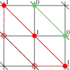
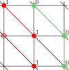
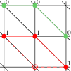
The proof is similar to the one of Theorem 1 but involves some additional technical points.
Proof.
We assume as before that . Like the CA of the previous section, the new process that we have defined has the property not to break up or connect different clusters. Furthermore, if we consider a -cluster and the smallest rectangle in which it is contained, we can check again that the -cluster will never go beyond this rectangle. As before, we only need to prove that any finite -cluster disappears almost surely in finite time to conclude the proof. We consider a realisation of the trajectory of the IPS with initial density . We associate to any finite -cluster the point , where the order is the lexicographic order on the coordinates (we set ). The point is thus the upmost point of among its rightmost points. Let us consider at time some finite -cluster . We denote by the state of this cluster at time .
Claim. The value is nonincreasing. Moreover, if is such that , then there exists almost surely a time such that .
Let us prove the claim. Let us denote by a configuration attained at some time , and let . By definition of , if a cell of coordinate is connected to a cell of , then . Either we have also and the cell will not flip. Or , but in this case, since does not belong to , and the cell of to which is connected is necessarily . So, and , once again by definition of . Depending on the value of , either rule 1 or rule 2 forbids the cell to flip. In the same way, we can prove that if a cell of coordinate is connected to , then it is not allowed to flip. This proves that is nonincreasing. In order to prove the second part of the claim, we need to show that the cell will almost surely be flipped in finite time. By definition of , we know that . The cell will thus be allowed to flip, except if and . But in that case, the cell will end up flipping, except if , and so on. Let . If for each , the cells of are in the state , then none of the cell is allowed to flip (see Figure 2.a). But recall now that the initial measure is . There exists almost surely an integer such that the initial state of the cell is not . Let be the smallest integer whose value at time is not . Then, one can easily check that is non-increasing, and that it reaches in finite time. Thus, the cell ends up flipping and we have proved the claim.
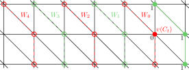
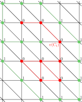
The example of Figure 2.b illustrates how the proof works. Here, no cell of the cluster is allowed to flip, but since the cells on the right and on the top of cannot flip either, does not increase. The cell at the left of will end up flipping, and will then be allowed to flip.
Since we know that a -cluster cannot go beyond its enveloping rectangle, a direct consequence of the claim is that any -cluster disappears in finite time. This allows us to conclude the proof in the same way as for the majority cellular automaton. ∎
4 Classifying the density on regular trees
Consider the finitely presented group . The Cayley graph of is the infinite -regular tree. For , we also consider the free group with generators, that is, . The groups and are not isomorphic, but they have the same Cayley graph.
4.1 Shortcomings of the nearest neighbour majority rules
For odd values of , a natural candidate for classifying the density is to apply the majority rule on the neighbours of a cell. But it is proved that neither the CA (see [12] for and 7) nor the IPS (see [11] for ) classify the density.
For , a natural candidate would be to apply the majority on the four neighbours and the cell itself. We now prove that it does not work either.
Proposition 3.
Consider the group Consider the majority CA or IPS with neighbourhood . For , the trajectories do not converge weakly to a uniform configuration.
Proof.
If , then we claim that at time , there are almost surely infinite chains of zeros and infinite chains of ones that are fixed. Let us choose some cell labelled by . Consider the (finite or infinite) subtree of 1’s originating from this cell viewed as the root. If we forget the root, the random tree is exactly a Galton-Watson process. Indeed, the expected number of children of a node is and since , this Galton-Watson process survives with positive probability. Consequently, there exists almost surely an infinite chain of ones at time somewhere in the tree. In the same way, since , there exists almost surely an infinite chain of zeros. ∎
As for , we get round the difficulty by keeping the majority rule but choosing a non-symmetrical neighbourhood.
4.2 A rule that classifies the density on
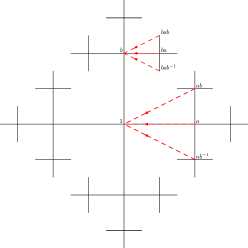
In this section, we consider the free group see Fig. 3 (a).
Theorem 3.
The cellular automaton defined by:
for any , classifies the density.
Proof.
We consider a realisation of the trajectory of the CA with initial distribution . Let us denote by the random variable describing the state of the cell at time . Since the process is homogeneous, it is sufficient to prove that converges almost surely to if and to if . Let us denote by the function that maps a given to the probability that when are three independent Bernoulli random variables of parameter . An easy computation provides , and one can check that the sequence converges to if and to if .
We prove by induction on that for any , the family consists of independent Bernoulli random variables of parameter . By definition of , the property is true at time . Let us assume that it is true at some time , and let us fix some . Two different elements of can be written as the majority on two disjoint triples of . The fact that the triples are disjoint is a consequence of the fact that is a code: a given word written with the elementary patterns can be decomposed in only one way as a product of such patterns. By hypothesis, the family is made of i.i.d. Bernoulli variables of parameter , so the variables of are independent Bernoulli random variables of parameter . Consequently, the process classifies the density on .∎
Let us mention that from time , the field is not i.i.d. For example, and are not independent since both of them depend on .
On , one can either apply Prop. 2 to obtain a cellular automaton that classifies the density, or define a new CA by the following formula: and check that it is also classifies the density.
It is also possible to adapt the above proof to show that the IPS with the same local rule also classifies the density.
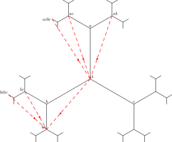
4.3 A rule that classifies the density on
We now consider the group .
Theorem 4.
The cellular automaton defined by:
for any , classifies the density.
Proof.
The proof is analogous to the previous case. We prove by induction on that for any , that the family consists of independent Bernoulli random variables of parameter , the key point being that is a code.∎
Once again, as explained in Prop. 2, since we have a solution on , we obtain a CA that classifies the density for any by applying exactly the same rule. The corresponding IPS on also classifies the density.
5 Classifying the density on
The one-dimensional case appears as much more difficult than the other cases and we are not aware of any solution to the density classification problem on . However, if we slightly change the formulation of the problem, simple solutions do exist. We first give one such modification and then go back to the original problem and describe three models, two CA and one PCA, that are conjectured to classify the density. We also provide some preliminary analytical results as well as experimental confirmations of these results by using numerical simulations.
In the examples below, the traffic cellular automaton, rule 184 according to Wolfram’s notation, plays a central role. It is the CA with neighborhood and local function traf defined by:
This CA can be seen as a simple model of traffic flow on a single lane: the cars are represented by 1’s moving one step to the right if and only if there are no cars directly in front of them. It is a density-preserving rule.
5.1 An exact solution with weakened conditions
On finite rings, several models have been proposed that solve relaxed variants of the density classification problem. We concentrate on one of these models introduced in [15]. The original setting is modified since the model operates on an extended alphabet, and the criterium for convergence is also weakened. Modulo this relaxation, it solves the problem on finite rings . We show the same result on .
Proposition 4.
Consider the cellular automaton on the alphabet , with neighbourhood , and local function defined by:
| (3) |
The projections converge to if and to if .
Intuitively, the CA operates on two tapes: on the first tape, it simply performs the traffic rule; on the second tape, what is recorded is the last occurrence of two consecutive zeros or ones in the first tape. If , then, on the first tape, there is convergence to configurations which alternate between patterns of types and . Consequently, on the second tape, there is convergence to the configuration . We formalise the argument below.
Proof.
Let be the traffic CA, see above. Following an idea of Belitsky and Ferrari [1], we define the recoding by . Consider , the recodings of the trajectory of the CA originating from . There is a convenient alternative way to describe . It corresponds to the trajectories in the so-called Ballistic Annihilation model: and are interpreted as particles that we call respectively positive and negative particles. Negative particles move one cell to the left at each time step while positive particles move one cell to the right; and when two particles of different types meet, they annihilate.
Consider the Ballistic Annihilation model with initial condition for . The density of negative particles is , while the density of positive particles is . During the evolution, the density of positive particles decreases to 0, while the density of negative particles decreases to . In particular, the negative particles that will never disappear have density (see [1] for details). We can track back the position at time 0 of the “eternal” negative particles. Let be the (random) position of the first eternal particle on the right of cell . After time , the column 0 in the space-time diagram contains only or values. This key point is illustrated in the figure below.
![[Uncaptioned image]](/html/1111.4582/assets/x8.png)
We now go back to the traffic CA with initial condition distributed according to for and concentrate on two consecutive columns of the space-time diagram. The property tells us that after some almost surely finite time, the columns contain only the patterns , or
For the CA defined by Eq. 3 with an initial condition distributed according to a measure satisfying for , the above key point gets translated as follows: in any given column of the space-time diagram, after some a.s. finite time, the column contains only the letters or . In particular, converges weakly to if . ∎
5.2 Density classifier candidates on
The GKL cellular automaton.
The Gács-Kurdyumov-Levin (GKL) cellular automaton is the CA with neighbourhood defined by
for any
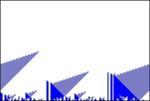
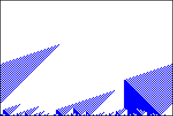
The GKL CA is known to be one of the best performing CA for the density classification on finite rings (see Fig. 4). It has also been proven to have the eroder property: if the initial configuration contains only a finite number of ones (resp. zeros), then it reaches (resp. ) in finite time, see [9].
Kari traffic cellular automaton.
This CA is defined by the composition of the two following rules applied sequentially at each time step: (a) apply the traffic rule, (b) change the into a in every pattern and the into a in every pattern (see Fig. 4).
Like GKL, Kari traffic CA has a neighbourhood of radius . Both CA also share the combined symmetry consisting in swapping and and right and left. Kari traffic has also the eroder property and it appears to have comparable qualities to GKL concerning the density classification task, see [15]. Kari traffic CA is closely related to Kurka’s modified version of GKL [13].
 |
 |
| GKL, | GKL, |
 |
 |
| Kari, | Kari, |
The majority-traffic probabilistic cellular automaton.
The majority-traffic PCA of parameter is the PCA of neighbourhood and local function:
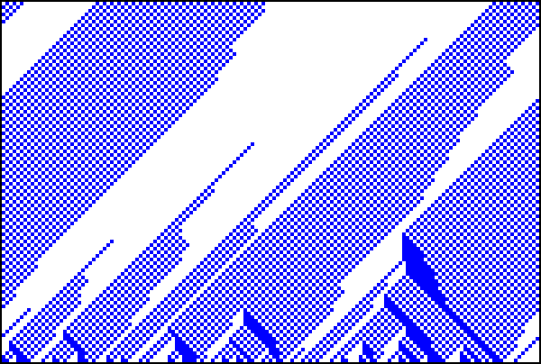
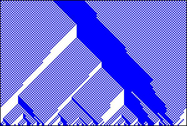
In words, at each time step, we choose, independently for each cell, to apply the majority rule with probability and the traffic rule with probability (see Fig. 5).
The majority-traffic PCA has been introduced by Fatès [4] who has proved that it “classifies” the density on a finite ring with an arbitrary precision: for any and any , there exists a value of the parameter such that on , the PCA converges to the right uniform configuration with probability greater than .
Conjecture 1.
The GKL CA, the Kari traffic CA, and the majority-traffic PCA with (for some ) classify the density.
5.3 Invariant Measures
Following ideas developed by Kurka [13], we can give a precise description of the invariant measures of these PCA.
Proposition 5.
For the majority-traffic PCA and for Kari traffic CA, the extremal invariant measures are and . For GKL, on top of these three measures, there exist extremal invariant measures of density for any .
Proof.
Majority-traffic PCA. Let us consider the majority-traffic PCA of parameter . We denote by the cylinder set of all configurations satisfying for . Let be any shift-invariant measure. An exhaustive search shows that if at time , we observe the cylinder then there are only eight possible cylinders of size at time , that are:
If we weight each cylinder by the probability to reach from them, we obtain the following expression:
Since the measure is supposed to be shift-invariant, we do not need to specify the position of the cylinders: we denote by the value which does not depend on . Gathering the terms with the same coefficient, we have:
Some more rearrangements provide:
This proves that the sequence is non-increasing. Let us assume that . Then, .
Let us consider the cylinder for some . If we apply the majority rule on each cell except on the second cell from the left, then after iterations, we reach the cylinder . Since this occurs with a positive probability, we obtain that for any . This provides: for any . Consequently, . From a cylinder of the form , if we choose to apply the majority rule on each cell, then we reach the cylinder in steps. Thus, for any . It follows that can be written as the sum of two invariant measures, where charges only the subshift and the subshift . Let us assume that (which is the case for ). In the same way that we have computed , we can compute , and we obtain:
By hypothesis, , so that the last equality implies that .
In all cases, if is a shift-invariant measure such that , then and .
Kari traffic CA. If at time , we observe the pattern at position , then, at time , that is to say before the application of Kari’s CA, this same pattern was present at position . Indeed, one can check that none of the cell of the pattern can have been obtained by the transformation (b) (see the definition of Kari traffic CA), so that one has just to consider the possible history of by the traffic CA. In the same way, one can prove that if at time , we observe the pattern at position , then, at time , this same pattern was present at position . Let be a shift-invariant measure such that , where denotes Kari traffic CA. A consequence of the result on the patterns and that we have just described is that for any and any . But since , we obtain for any word on the alphabet . Once again, we can write where and are two invariant measures defined on and .
Let us consider a configuration of , that is, without the pattern . By the traffic rule, each of the configuration will move one cell to the left. Then by rule , if a is at distance greater than from the next on its right, it is erased by rule (b). The result follows.
GKL. Any word that is a concatenation of the patterns and is a fixed point of the GKL cellular automaton: if , then either or so that and if , then either or so that . As a consequence, GKL has extremal invariant measures of density for any . ∎
To summarize, the majority-traffic and Kari traffic CA have a simpler set of invariant measures. It does not rule out GKL as a candidate for solving the density classification task, but rather indicates that it could be easier to prove the result for majority-traffic or Kari traffic CA.
5.4 Experimental results
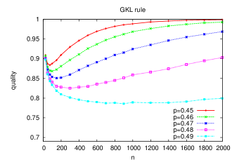
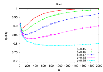
Conjecture 1 was first motivated by the observation of the space-time diagrams, see Fig. 4 and 5. We provide some numerical results that support this conjecture. For a given ring size , we generate an initial configuration by assigning to each cell the state 1 with a probability and the state 0 with probability . Let us denote by the actual density of in the configuration . We let the system evolve until it reaches a fixed point or and see if the fixed point is for and for . The quality corresponds to the proportion of good classifications on a given ring of size .
 |
 |
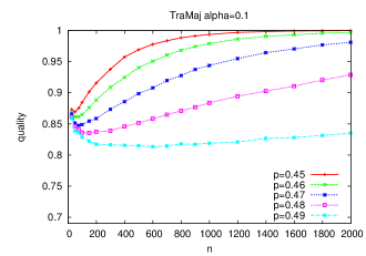 |
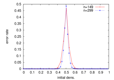
Figure 6 shows the evolution of , each value of being evaluated over 100 000 samples. For the three rules, the plots are in agreement with the hypothesis that the asymptotic value of is 1. From a qualitative point of view, we observe that for all values of the quality decreases before increasing, but this is only a border phenomenon for very small ring sizes. We also observe that when the initial density increases from to , the value of needed to attain a given quality increases dramatically. For , the change of derivative of the curve becomes hardly visible. However, our belief is that will approach one as the lattice size grows, no matter how close is to the critical density . To see why this holds, consider the error rate obtained as the probability to make a bad classification when the initial configuration is equal to . We experimentally observed that, as grows, the function , which is defined for values with , approaches a Bell curve whose mean is centred on and whose tail progressively approaches the 0-axis (see Fig. 7). At the same time, for a fixed , the probability that the initial configuration has a density of ones equal to follows a binomial distribution of parameter . We can thus calculate the global error rate with . Intuitively, it can be seen that as grows to infinity, the two distributions and progressively separate as their mean value is different and their variance approaches 0. As a consequence, for larger values of , the value progressively vanishes and the quality approaches 1.
By contrast, there are other PCA, such as the rule which was originally studied by Fukś [6], and which consists in doing a copy of the right or left neighbour with a fixed probability , and the identity otherwise. This rules preserves the density in average at each time step for finite rings (see details in [4]). As a consequence, we have which implies that the increase of does not improve the average performance of the system. In the infinite case, the preservation of the density is exact and can not allow the system to classify the density. We experimentally observed the same qualitative behaviour for the rule used by Schüle [18] or for the Majority-Traffic rule for . We believe that there exists a strong relationship between the asymptotic behaviour of the rule on finite rings and the ability to classify the density on .
5.5 Link with the positive rates “conjecture”
The difficulty of classifying the density on is related to the difficulty of the ergodicity problem on . By definition, a PCA or an IPS has positive rates if all its local probability transitions are different from 0 and 1. In , there exist positive rates PCA and IPS that are non-ergodic (for instance, a “positive rates version” of Toom’s rule [3]). It had been a long standing conjecture that all positive rates PCA and IPS on are ergodic. Gács disproved the conjecture by exhibiting a complex counter-example with several invariant measures, but with an alphabet of cardinality instead of 2 [8]. If we knew a process that classifies the density on , it could pave the way to exhibit simple examples of positive rates processes that are non-ergodic.
References
- [1] Belitsky, V., Ferrari, P.A.: Invariant measures and convergence properties for cellular automaton 184 and related processes. J. Stat. Phys. 118(3-4), 589–623 (2005)
- [2] Cox, J.T., Durrett, R.: Nonlinear voter models. In: Random walks, Brownian motion, and interacting particle systems, Progr. Probab., vol. 28, pp. 189–201. Birkhäuser Boston, Boston, MA (1991)
- [3] Dobrushin, R., Kri︠u︡kov, V., Toom, A.: Stochastic cellular systems: ergodicity, memory, morphogenesis. Nonlinear science, Manchester University Press (1990)
- [4] Fatès, N.: Stochastic Cellular Automata Solve the Density Classification Problem with an Arbitrary Precision. In: 28th International Symposium on Theoretical Aspects of Computer Science (STACS 2011). vol. 9, pp. 284–295 (2011)
- [5] Fontes, L.R., Schonmann, R.H., Sidoravicius, V.: Stretched exponential fixation in stochastic Ising models at zero temperature. Comm. Math. Phys. 228(3), 495–518 (2002)
- [6] Fukś, H.: Nondeterministic density classification with diffusive probabilistic cellular automata. Phys. Rev. E 66 (2002)
- [7] Gács, P.: A Toom rule that increases the thickness of sets. J. Statist. Phys. 59(1-2), 171–193 (1990)
- [8] Gács, P.: Reliable cellular automata with self-organization. J. Statist. Phys. 103(1-2), 45–267 (2001)
- [9] Gonzaga de Sá, P., Maes, C.: The Gacs-Kurdyumov-Levin automaton revisited. J. Statist. Phys. 67(3-4), 507–522 (1992)
- [10] Grimmett, G.: Percolation, Grundlehren der Mathematischen Wissenschaften, vol. 321. Springer-Verlag, Berlin, second edn. (1999)
- [11] Howard, C.D.: Zero-temperature Ising spin dynamics on the homogeneous tree of degree three. J. Appl. Probab. 37(3), 736–747 (2000)
- [12] Kanoria, Y., Montanari, A.: Majority dynamics on trees and the dynamic cavity method. Ann. Appl. Probab. (To appear)
- [13] Kurka, P.: Cellular automata with vanishing particles. Fund. Inform. 58(3-4), 203–221 (2003)
- [14] Land, M., Belew, R.K.: No perfect two-state cellular automata for density classification exists. Phys. Rev. Lett. 74, 5148–5150 (1995)
- [15] Le Gloannec, B.: Around Kari’s traffic cellular automaton for the density classification. Master’s thesis ENS Lyon (2009)
- [16] Liggett, T.M.: Interacting particle systems. Classics in Mathematics, Springer-Verlag, Berlin (2005), reprint of the 1985 original
- [17] Packard, N.H.: Dynamic Patterns in Complex Systems. World Scientific, Singapore (1988)
- [18] Schüle, M., Ott, T. and Stoop, R.: Computing with Probabilistic Cellular Automata, ICANN ’09: Proceedings of the 19th International Conference on Artificial Neural Networks, 525–533 (2009)