Effect of discrete time observations on synchronization in Chua model and applications to data assimilation
Abstract
Recent studies show indication of the effectiveness of synchronization as a data assimilation tool for small or meso-scale forecast when less number of variables are observed frequently. Our main aim here is to understand the effects of changing observational frequency and observational noise on synchronization and prediction in a low dimensional chaotic system, namely the Chua circuit model. We perform identical twin experiments in order to study synchronization using discrete-in-time observations generated from independent model run and coupled unidirectionally to the model through , and separately. We observe synchrony in a finite range of coupling constant when coupling the and variables of the Chua model but not when coupling the variable. This range of coupling constant decreases with increasing levels of noise in the observations. The Chua system does not show synchrony when the time gap between observations is greater than about one-seventh of the Lyapunov time. Finally, we also note that prediction errors are much larger when noisy observations are used than when using observations without noise.
The possibility of using chaotic synchronization for data assimilation is entertained. In particular, synchronization observed for two chaotic Chua models under unidirectional coupling is shown to be of relevance for forecasting using data assimilation techniques. Our results indicate that prediction method employed in the present is extremely sensitive to observational frequency, Lyapunov exponent and the phase at which the coupling is switched off.
I Introduction
Data assimilation (DA) is a powerful and versatile method for combining partial, noisy observational data of a system with its dynamical model, generally numerically implemented, to generate state estimates of nonlinear, chaotic systems. A variety of data assimilation methods, broadly separated into deterministic or probabilistic methods, have been developed over the past few decades and used mainly in the earth sciences.book:lewisvarahan06 ; book:park08 ; Kalnay03 ; book:malanotte96 ; Ben01 ; book:evensen ; PhysicaD:Ide On the other hand, when two or more chaotic systems are coupled, they may adjust the properties of their motion due to coupling in such a way that their evolution becomes synchronized. Several types of coupling, unidirectional, mutual, common driving, etc., and their effects in the form of a variety of synchronizations such as identical, generalized, phase, lag, amplitude, etc., as well as applications of synchronizations have been and continue to be a very active area of research.prl:pecora ; book:pikovosky
We will be interested in this paper with sequential data assimilation, which incorporates observations sequentially in time. This method can be thought of as synchronization through unidirectional coupling, with observations acting as the master system and the numerical model acting as the slave system.prl:pecora ; atmos:yang ; npg:Duane ; JGR:Szendro In fact, this is exactly the nudging method for assimilation, suggested first in meteorology,mwr:hoke and later used for a number of different studies.jgr:verron ; tellus:stauffer ; mwr:bao ; jaot:wang ; ngp:aurox Recent studies show that such techniques can also be used for assimilating data in order to track complex spatio-temporal dynamics of excitable media,chaos:berg and forecast the state of a time-delayed high-dimensional system, e.g., in chaotic communication.prl:cohen Synchronization based DA method may be useful for small or mesoscale predictions, specially when observations are frequent and coupled to a small number of variables.atmos:yang ; ngp:aurox This method is relatively fast and robust, and can be implemented easily.Oceanography:Stammer
Two of the main characteristics of the observational data used in earth sciences applications is that they are discrete in time and are noisy. The main aim of this paper is to study synchronization with these characteristics in mind, as we explain below.
-
1.
It has been observed recentlyDynAtmOcean:ide ; jhydro:walker ; waterres:walker ; tellus:apte that the time period between two observations is one of the important factors which significantly affect conventional DA schemes. Though frequent updates may produce better results depending on the quality of the model as well as the observations, they increase the burden of computational cost.advspaceres:Riishojgaard Since the choice of observational frequency depends on many factors such as cost and ease of observations, it is important to understand in detail how the time period between observations affects the accuracy of predictions which in turn depends on the accuracy of the data assimilation.
For these reasons, we investigate the effect of varying observational frequency, i.e., the gaps between the observations, on discrete time synchronization – this discussion forms the first part of the paper. As expected, we find that observations which are farther apart lead to poorer synchronization and consequently low accuracy of prediction. We also find that there is a certain threshold, which in the system we study is roughly of the order of the inverse of Lyapunov exponent of the system, such that using observations with a time period greater than that threshold leads to no synchronization.
-
2.
It is of course well known that the observational noise plays crucial role in data assimilation as well as in synchronization.PRL:Neiman ; PRL:Teramae ; PRE:Guan Thus we also carry out the study described in the above paragraph with noisy observations with different noise levels, in order to investigate the effect of noise on synchronization. The discussion of these results forms the second part of the paper. Again as expected, the increase in noise leads to poorer synchronization and prediction.
We present these results in detail in section III and a discussion of these results along with directions for further studies are presented in section IV.
In order to investigate the effects of these two aspects, we perform the so-called “identical twin experiments”tellus:talagrand81 as follows. We generate observations using a known trajectory, called the “true” trajectory of a numerical model. We use these observations (master) to try to synchronize the same numerical model starting with a different initial condition (slave). We quantify the “degree of synchronization” by calculating the root mean square (RMS) error of the slave trajectory with respect to the true trajectory, leaving out the first half of the time-span, in order to get rid of transients. We assess the effect on predictions by calculating the RMS error over certain time-spans after the synchronization is stopped and the slave model is let to run by itself. Currently we are investigating the effect of these two factors, the time period between observations and the noise level, on data assimilation methods such as ensemble Kalman filter (ENKF).book:evensen
The dynamical model we use is that of a chaotic Chua circuit.IJBC:chua ; pre:singla One of the main reason for this choice is that in future we would like to use the actual data from the circuit experiments being currently performed by two of the authors.pre:singla This model is described in detail in the following section.
II Chua circuit model and synchronization
To study synchronization we have used the Chua model used in Ref. pre:singla, . The model of the circuit is made dimensionless by substituting , where , and and are the resistance and capacitor used in the circuit respectively. The dimensionless model is given by.
| (1) |
where
and and are the parameters whose values depend on the capacitors, resistances and inductor used in the circuit.pre:singla The resistance is the control parameter of the system. Depending on R, the system shows chaotic or regular behavior. In the present study, we have chosen , , and . The model was integrated using the fourth order Runge-Kutta numerical scheme with integration step , and the output of the model has been expressed in terms of real time rather than in terms of the dimensionless time .
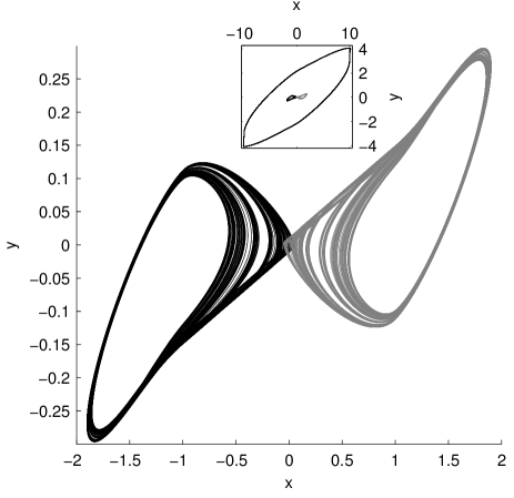
The model equations show three attractors depending upon the initial conditions as shown in Fig. 1(inset), and zoomed version of the smaller attractors by black and gray plots. As the basin of attractors is not known, it is not possible to tell a priory which initial condition will lead to a particular attractor. Generally, for high values of initial condition (approximately greater than in absolute value), system goes to the large limit cycle attractor [inset of Fig. 1], and for smaller initial conditions, system stays on any of the two small attractors [Fig. 1]. As the larger attractor is not of experimental interest, the dynamics on this attractor is considered as divergent dynamics.
In the present simulation, we have used for which the system shows chaotic behavior. The “true” (or master) initial condition is chosen such that the trajectory stays on any one of the small attractors depending upon the initial conditions. The largest Lyapunov exponent () is positive ( bits/msec), and corresponding Lyapunov time is . was estimated using Rosenstein techniques physicaD:Rosenstein and is consistent with the earlier results.JCktSystComp:parlitz
In order to generate any one set of observations, we first simulated a long trajectory on one of the smaller attractors. We refer to such a trajectory as “truth” in keeping with other data assimilation literature. Next, we sub-sampled this trajectory to extract several sets of discrete-time equispaced observations with varying time interval between the observations, which will henceforth be denoted by . For the present study, observations were generated with four different values of , namely, , , , and sec. Noisy observations were created by adding noise of particular intensity () to these discrete-time observations, where was chosen to be a specified fraction of the standard deviation of the attractors. The results presented in Sec. III are for one specific set of observations, but the qualitative features of these results were found to be identical when we used observational sets generated from many different initial conditions.
II.1 Master-slave coupling
The model (slave) was unidirectionally coupled with discrete-time observations (master) at times as follows.
| (2) |
where, , and represent the , , and coupling. In the case of continuous time observations which is also discussed below, the slave is coupled to the master directly, by replacing the summations of delta functions in the above equations by terms such as . We have quantified synchronization using RMS error of the difference of the synchronized and true trajectory over the last half of the trajectory, and the quality of prediction is again quantified by the RMS error with respect to truth over varying time periods, as discussed in detail below. The results about synchronization and prediction for different and noise level (), and a comparison of these results with the case of continuous time synchronization are presented in the next section.
III Results
The main aim of this section is to discuss the effects of the observational time period and the observational noise variance on the root mean square of the difference between the slave system and the master, both during the time period in which the slave is coupled to the master (synchronization phase) and after the coupling is switched off (the prediction phase).
III.1 Synchronization with observations without noise ()
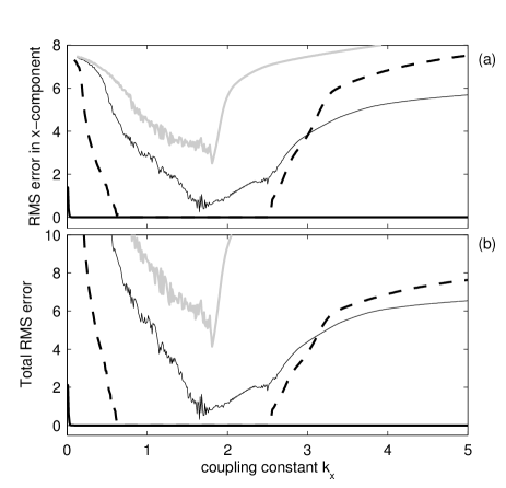
In order to investigate the performance of the synchronization, we have first studied the case of coupling only the -component, i.e. setting in Eqns. 2 while is varied from zero to higher values. We quantify synchronization of each components by calculating the RMS error of the component-wise difference of master and slave trajectories, and also the total RMS error. For continuous case, the slave model synchronizes with the master within a very short time. Solid lines in Fig 2 (a) and (b) show the RMS errors in -component and total errors respectively. They show that the system started synchronizing around , and achieved full synchronization around as the RMS errors are almost zero. The system remained in synchronized state even at higher values of .
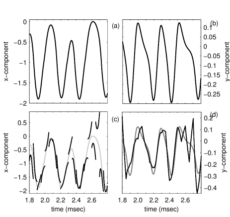
Synchronization with -component observations at discrete time is shown in Fig. 2. In this figure, the dashed-lines show the RMS errors when -observation were recorded with sec, which is approximately 18 times less than . The figure also shows that the model started synchronizing around with the observations and achieved full synchronization around . For model diverges from the observations. So the range of the coupling for which there is synchrony has become finite when observations were taken at a finite interval. Synchrony is also clear from the plots of and time series of the observational trajectories and slave trajectories shown in Fig. 3. They show the model (gray lines) gets perfectly synchronized with the observational trajectory (black lines).
Note that RMS error above approx. indicates a loss of synchronization, hence effectively synchronization is obtained only for the first two of these cases, i.e., continuous time observations and with sec.
Black thin solid lines [Fig 2] show the RMS errors, when the observations were taken with sec. (). In this case errors decreased slowly with and showed partial synchronization only in a very small range of around . The time series at in plots (c) and (d) of Fig. 3 show such partial synchrony between the observed trajectory (gray lines) and the slave model (black line) for sec. The behaviour of the -component was similar to that of the . For sec, the RMS error is least around but even in this case, it is far from being synchronized. These results show that is an important factor in synchronization that must be considered in DA experiments.
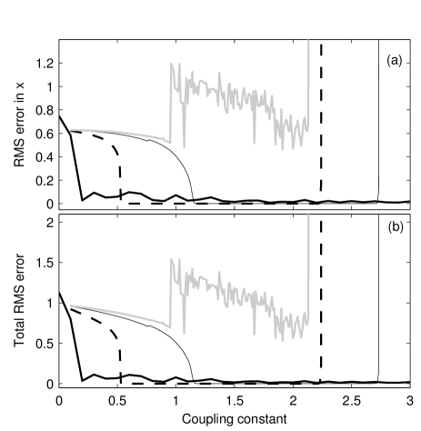
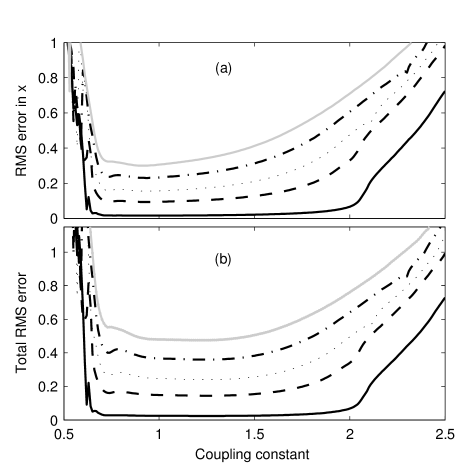
When -component was observed, i.e., when we set and vary , the model showed synchrony for different range of than that was for observations. In Fig. 4, the solid lines show the RMS errors in (a) -component and (b) total RMS error for continuous observation case. Around the model achieved synchrony and remains in this state even at higher values of . For sec (dashed lines), slave system achieved full synchronization around , and remains synchronized for . When (thin solid), the synchronization region shifts to . Similar to -observation case, there is no synchronization for the -observation with (gray line) and above. Thus we see that the -component is a more dominant dynamical variable than the -component.
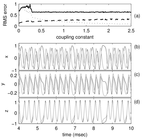
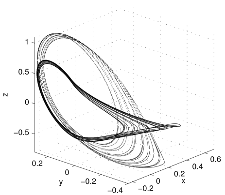
When model was coupled with master through -observations (), there was no synchronization even for the continuous observations case. Panel (a) of Fig 5 shows the RMS errors in (solid line), (dashed line), and (dotted line) components as is varied. This is also clear from the plots of , , and time series of the master (gray) and slave (solid) shown in panels (b), (c), and (d), respectively. The difference between the master (solid line) and slave (dotted line) is also clear from the attractors shown in Fig 6. A possible explanation for not having synchronization with coupling is that this variable may not contain sufficient information about the dynamics. Hence in the current regime of the Chua system and contain useful information for synchronization but not the -component.atmos:yang Finally as the model did not show any synchrony for continuous case, obviously we did not get any synchrony with discrete time observations either.
III.2 Synchronization with noisy observations
To study the effect of noise on synchronization, we added noise to the -component of observation with , which is used in Sec. III.1, and repeated the same experiments. We have not performed any experiments with noisy continuous time observations, since we are only considering deterministic models.
In Fig. 7 (a) and (b), the solid lines represent the RMS errors in -component and total error respectively when added noise intensity is . In this case, we got synchrony in the range of , and the model started desynchronizing around as shown in Figs. 7. So the noisy observations squeeze the k range further. With increase in overall range remained almost same. In Figs. 7 solid, dashed, dotted, dashed-dotted, and gray lines are the RMS errors when , , and respectively.
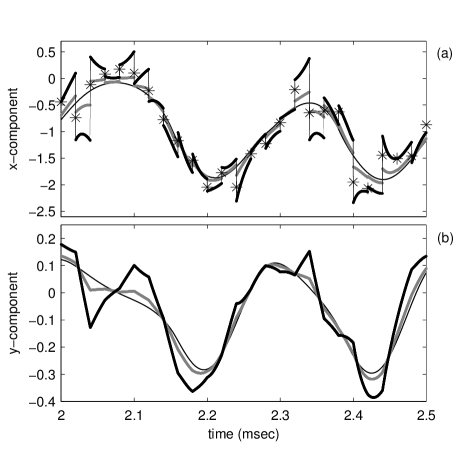
Effect of the noise is also clear from the time series plots. Fig. 8 shows the time series of the observation (thin solid line) and slave trajectories for (thick gray) and (thick solid line). They show that the deviation of the slave trajectories from the observed one increases with increasing noise level. But -component deviate lesser than and -component (not shown). It is also observed that the RMS errors increases almost linearly (not shown here) with increases in .
III.3 Prediction with truths and noisy observation
In this section we consider the use of the slave model for prediction. This is done in the following manner. We couple the observations with the slave system through Eqs. (2) for a long time period, in particular, until msec in our numerical experiments. Then we switch off the coupling, i.e., use Eqs. (1) for the slave beyond this time. The RMS errors described below are calculated over varying time periods, which are called the forecast horizons . We present the results for -observations with and since larger do not show any synchronization.
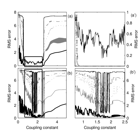
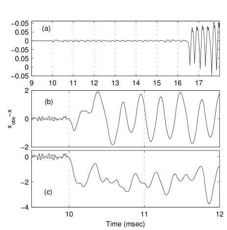
In Fig. 9 the prediction RMS errors in -component has been shown for the range of . The - and - components follow the same qualitative trend. Thick-solid, gray, dotted, dash-dotted and thin solid lines in Fig. 9 are the RMS errors for , and respectively, where boxed regions of Fig. 9 (a) has been zoomed in Fig. 9 (a′). We see that for slave system predicts well, i.e., the RMS errors are small, but when prediction diverges from true trajectory. Figs 9 (a′) [thin solid line] show that RMS error at is significantly large. Fig. 11 (a) show that slave model becomes completely uncorrelated with the master around .
Another important observations from our numerical experiments is that the forecast horizon for which the slave shows small RMS error with respect to the master is highly dependent on the state of the system at which the coupling is turned off. This is because the uncertainty growth rate is different on different parts of the attractor. pla:Ziehmann
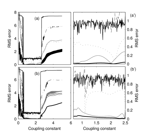
When noisy observations are coupled with the slave system, the divergence of the slave from the master is rapid once the coupling is switched off. Fig. 10 shows errors in -components when noise with intensity (top panels) and (bottom panels) is added to the observations. We have seen that for (not shown in figure), there is a range of coupling constants for which the prediction RMS error is small enough to give good prediction. For larger , the slave model become uncorrelated with the master and predictions cannot be obtained. This is the case for both cases of the observations with and noise. Divergence is also clear from the difference of time series of with of noise [Fig. 11 (b)] and of noise [Fig. 11 (c)] respectively.
IV Conclusion
This paper is devoted to the study of discrete-time unidirectional synchronization, with specific emphasis on aspects which are of relevance to data assimilation problems. In particular we consider the observations of a system, in this case the chaotic Chua system of Eqs. (1), to be the master coupled unidirectionally to the slave system of Eqs. (2) and examine how the slave system synchronizes with the master as we change various characteristics of the observations. The main discussion is focused on studying the effects of changing observational period, i.e. the time between the observations , and observational noise levels . Some of the main results as well as directions for future research which we are currently pursuing are discussed below.
We obtained synchronization with continuous time observations of the - and -components of the system, but not with -component observations. When discrete observations with finite were used, Chua model showed synchrony for a finite range of coupling constants, and this range decreases with increase in and noisy observations. The study also shows that the system shows synchrony only when the observations were taken with much less than (almost ) while for larger there is no synchronization between the master and the slave.
In many cases of practical interest in earth sciences, data assimilation is used as a tool to improve prediction of the observed as well as unobserved components of the system. With this in mind, we also study the prediction errors over different forecast horizons after the coupling between the observations and the slave is turned off. We see that in the cases when synchronization errors are small, the prediction errors even for forecast horizons far beyond the Lyapunov timescale are small. This happens only for the case of observations which are not noisy. When using observations even with a very small noise, the slightly higher synchronization errors coupled with chaotic nature of the system lead to loss of predictive power over forecast horizons which are a fraction of the Lyapunov timescale. These results indicates that the association of the Lyapunov exponent with predictability horizons has limited use.pla:Ziehmann These results also show the limitations of discrete-time synchronization with noisy observations and the importance of the study of other data assimilation techniques which systematically take into account the noise in the observations.
In synchronization choice of coupling constant is merely ad hoc and depends on a particular application. In case of data assimilation using similar techniques, e.g. nudgingngp:aurox , the choice of can be interpreted in terms of variational approach. In particular, Ref. ngp:aurox, shows, using the variational approach, that the optimal coupling constant is inversely proportional to observational noise covariance: , where is the covariance matrix of observational errors. As the range of on which model shows synchrony depends mainly on observed component and noise, we are investigating the possibility that a similar formulation may also be possible for synchronization to choose the appropriate . We will also be comparing the synchronization based methods with data assimilation techniques such as the ensemble Kalman filterbook:evensen and Bayesian methods.physd:apte07
Another ongoing investigation is to study the performance of these methods in the chaotic Chua model using real data from the circuitpre:singla . This study will give us an insight about the choice of coupling constants and observational time period, the effects of observational noise as well as of the errors in the numerical model.
Acknowledgments
AA and MN would like to thank the Indian National Centre for Ocean Information Services for financial support through Project No. INCOIS/93/2007.
References
- (1) J. M. Lewis, S. Lakshmivarahan, and S. Dhall, Dynamic Data Assimilation: A Least Squares Approach, Encyclopedia of Mathematics and its Applications, Vol. 104 (Cambridge University Press, 2006).
- (2) Data Assimilation for Atmospheric, Oceanic and Hydrologic Applications, edited by S. K. Park and L. Xu (Springer, 2008).
- (3) E. Kalnay, Atmospheric modeling, data assimilation, and predictability (Cambridge University Press, 2003).
- (4) Modern Approaches to Data Assimilation in Ocean Modeling, edited by P. Malanotte-Rizzoli (Elsevier Science, 1996).
- (5) A. F. Bennett, Inverse modeling of the ocean and atmosphere (Cambridge University Press, 2002).
- (6) G. Evensen, Data Assimilation: the Ensemble Kalman Filter (Springer, 2009).
- (7) K. Ide and C. K. Jones, Physica D 230 (2007), nos. 1-2, Data Assimilation (special issue).
- (8) L. M. Pecora and T. L. Carroll, Phys. Rev. Lett. 64, 821 (1990).
- (9) A. Pikovsky, M. Rosenblum, and J. Kurths, Synchronization: A universal concept in nonlinear sciences, 1st ed., The Art of Computer Programming, Vol. 2 (Cambridge University Press, The Edinburgh Building, Cambridge CB2 2RU, United Kingdom, 2001).
- (10) S.-C. Yang, D. Baker, H. Li, K. Cordes, M. Huff, G. Nagpal, E. Okereke, J. V. ne, E. Kalnay, and G. S. Duane, J. Atmos. Sci. 63, 2340 (2006).
- (11) G. S. Duane, J. J. Tribbia, and J. B.Weiss, Nonlin. Processes Geophys. 13, 601 (2006).
- (12) M. A. R. Szendro, I. G. and J. M. Lopez, J. Geophys. Res. 114, D20109 (2009).
- (13) J. Hoke and R. A. Anthes, Mon. Weather Rev. 104, 1551 (1976).
- (14) V. J., J. Geophys. Res. 95(C7), 443 (1990).
- (15) D. R. Stauffer and J. W. Bao, Tellus 45A, 358 (1993).
- (16) B. J. W. and E. R. M., Mon. Weather Rev. 125, 1355 (1997).
- (17) W. J, J. Atmos. and ocean Technology 18, 1037 (1990).
- (18) D. Auroux and J. Blum, Nonlin. Processes Geophys. 15, 305 (2008).
- (19) S. Berg, S. Luther, and U. Parlitz, Chaos 21, 033104 (2011).
- (20) A. B. Cohen, B. Ravoori, T. E. Murphy, and R. Roy, Phys. Rev. Lett. 101, 154102 (2008).
- (21) D. Stammer and E. Chassignet, Oceanography 13, 51 (2000).
- (22) K. Ide and M. Ghil, Dynamics of Atmospheres and Oceans 27, 333 (1997).
- (23) J. P. Walker, G. R. Willgoose, and J. D. Kalma, J. Hydrol. 2, 356 (2000).
- (24) J. P. Walker, G. R. Willgoose, and J. D. Kalma, Water Resour. Res 38, 37 (2002).
- (25) A. Apte, C. Jones, and A. M. Stuart, Tellus A 60, 336 (2008).
- (26) L. P. Riishojgaard, I. Stajner, and G.-P. Lou, Adv. SpaceRes. 25, 1063 (2000).
- (27) A. Neiman, L. Schimansky-Geier, A. Cornell-Bell, and F. Moss, Phys. Rev. Lett. 83, 4896 (1999).
- (28) J. nosuke Teramae and D. Tanaka, Phys. Rev. Lett. 93, 204103 (2004).
- (29) S. Guan, Y.-C. Lai, and C.-H. Lai, Phys. Rev. E 73, 046210 (2006).
- (30) O. TALAGRAND, Tellus 33, 43 (1981).
- (31) L. O. Chua, L. Kocarev, K. Eckert, and M. Itoh, Int. J. Bifurcation Chaos 2, 705 (1992).
- (32) T. Singla, N. Pawar, and P. Parmananda, Phys. Rev. E 83, 026210 (2011).
- (33) M. T. Rosenstein, J. J. Collins, and C. J. D. Luca, Physica D 65, 117 (1993).
- (34) U. Parlitz, J. of Circuits, Systems, and Computers 3, 507 (1993).
- (35) L. A. S. C. Ziehmann and J. Kurths, Phys. Lett. A 271, 237 (2000).
- (36) A. Apte, M. Hairer, A. Stuart, and J. Voss, Physica D 230, 50 (2007).
- (37) L. M. B. Christopher K. Wikle, Physica D 230, 1 (2007).
- (38) N. F. Rulkov, M. M. Sushchik, L. S. Tsimring, and H. D. I. Abarbanel, Phys. Rev. E 51, 980 (1995).
- (39) G. Evensen, Ocean Dynamics 53, 343 (2003).
- (40) J. L. Anderson, Mon. Weather Rev. 129, 2884 (2001).
- (41) .
- (42) J. P. Walker, G. R. Willgoose, and J. D. Kalma, Water Resour. Res 38, 37 (2002).
- (43) G. S. Duane and J. J. Tribbia, J. Atmos. Sci. 61, 2149 (2004).
- (44) A. Timmermann and F.-F. Jin, Predictability of coupled processes, Pre- dictability of Weather and Climate (Cambridge University Press, 2006) pp. 251–274.