Transverse Energy Density Fluctuations in the Color Glass Condensate Model

Berndt Müller Department of Physics, Duke University, Durham, NC 27708    Andreas Schäfer Institut für Theoretische Physik, Universität Regensburg, 93040 Regensburg, Germany
Abstract

We calculate the transverse correlation of fluctuations of the deposited energy density in nuclear collisions in the framework of the Gaussian color glass condensate model.

I Event-by-event fluctuations

The event-by-event fluctuations of the transverse emission pattern of hadrons in high-energy collisions of identical heavy nuclei have recently attracted much interest experimentally Alver:2007qw ; Sorensen:2008zk ; ALICE:2011vk ; Adare:2011tg ; ATLAS:2011hf ; Sorensen:2011fb ; Appelt:2011mw and theoretically Miller:2003kd ; Broniowski:2007ft ; Andrade:2008xh ; Shuryak:2009cy ; Alver:2010gr ; Petersen:2010cw ; Alver:2010dn ; Staig:2011as ; Holopainen:2010gz ; Qin:2010pf ; Schenke:2010rr ; Qiu:2011iv ; Bhalerao:2011yg ; Qin:2011uw ; deSouza:2011rp . When averaged over collision events, the azimuthal angular distribution of emitted hadrons around the beam axis is symmetric with respect to the plane perpendicular to the impact parameter vector 𝐛𝐛{\bf b} between the two nuclei [Au+Au or Cu+Cu at the Relativistic Heavy Ion Collider (RHIC) or Pb+Pb at the Large Hadron Collider (LHC)]. The event averaged angular distribution

dNd2pT=dNπdpT2(1+n=1vn(pT)cos(ϕp)),𝑑𝑁superscript𝑑2subscript𝑝𝑇𝑑𝑁𝜋𝑑superscriptsubscript𝑝𝑇21superscriptsubscript𝑛1subscript𝑣𝑛subscript𝑝𝑇subscriptitalic-ϕ𝑝\frac{dN}{d^{2}p_{T}}=\frac{dN}{\pi dp_{T}^{2}}\Big{(}1+\sum_{n=1}^{\infty}v_{n}(p_{T})\cos(\phi_{p})\Big{)}, (1)

where ϕpsubscriptitalic-ϕ𝑝\phi_{p} is the angle between 𝐩Tsubscript𝐩𝑇{\bf p}_{T} and 𝐛𝐛{\bf b}, is therefore completely characterized by the even Fourier coefficients vnsubscript𝑣𝑛v_{n}. The dominant coefficient, v2subscript𝑣2v_{2}, is called elliptic flow.

Owing to quantum fluctuations in the density distributions of the colliding nuclei and finite particle number effects on the distribution of emitted particles, the left-right symmetry is broken in individual collision events. The angular distribution can then be written in the form

dNd2pT=dNπdpT2(1+n=1vn(pT)cos(ϕp+ψn)),𝑑𝑁superscript𝑑2subscript𝑝𝑇𝑑𝑁𝜋𝑑superscriptsubscript𝑝𝑇21superscriptsubscript𝑛1subscript𝑣𝑛subscript𝑝𝑇subscriptitalic-ϕ𝑝subscript𝜓𝑛\frac{dN}{d^{2}p_{T}}=\frac{dN}{\pi dp_{T}^{2}}\Big{(}1+\sum_{n=1}^{\infty}v_{n}(p_{T})\cos(\phi_{p}+\psi_{n})\Big{)}, (2)

where ψnsubscript𝜓𝑛\psi_{n} describes the tilt angle of the “event plane” for each Fourier coefficient with respect to the reaction plane defined by the vector 𝐛𝐛{\bf b}. For even n𝑛n, ψnsubscript𝜓𝑛\psi_{n} is peaked around zero; for odd n𝑛n, ψnsubscript𝜓𝑛\psi_{n} is randomly distributed. The dominant odd coefficient, v3subscript𝑣3v_{3}, is known as triangular flow. The event averages of the amplitude of the coefficients vnsubscript𝑣𝑛v_{n} are found to be constant over a rather large pseudorapidity range (|η|2𝜂2|\eta|\leq 2) in Pb+Pb collisions at the LHC ATLAS:2011hf , indicating an approximately boost invariant origin.

The main dynamical source of event-by-event fluctuations in the coefficients vnsubscript𝑣𝑛v_{n} are believed to be nearly boost invariant fluctuations in the transverse distribution of the energy density at the beginning of the hydrodynamic expansion of the quark-gluon plasma formed in the nuclear collisions. The geometric anisotropy of these fluctuations then translates in an anisotropic transverse collective flow pattern, which manifests itself in anisotropic particle emission. In the color glass condensate model of energy deposition there are two obvious sources of fluctuations in the deposited energy density. One is geometric fluctuations of the position of nucleons in the colliding nuclei at the moment of impact, leading to transverse fluctuations in the density of field generating color charges. This mechanism has been studied widely and is usually described geometrically by the Monte-Carlo Glauber model Drescher:2006ca . The transverse correlation length of the fluctuations generated by this mechanism will be of the order of the nucleon radius.

The other source of energy density fluctuations are fluctuations in the color field strength for a given density of color charges. This mechanism has not been investigated quantitatively up to now. The transverse correlation length generated by color field fluctuations will be dictated by the single scale governing the physics of the color glass condensate, the saturation scale Qssubscript𝑄𝑠Q_{s}. Since Qs1superscriptsubscript𝑄𝑠1Q_{s}^{-1} is much smaller than the nucleon radius, the color field fluctuations can be expected to govern the microscopic structure of the transverse energy density fluctuations, which then is modulated on longer transverse scales by fluctuations in the nucleon density in the colliding nuclei.

Here we calculate the transverse correlation function of the deposited energy density in nuclear collisions in the framework of the Gaussian approximation to the color glass condensate originally proposed by McLerran and Venugopalan McLerran:1993ni ; McLerran:1993ka . In Section II we derive the two-point correlator of the energy density following the collision of two color glass condensates. In Section III we evaluate the resulting integrals and present numerical results for the correlation function for a representative choice of parameters.

II Energy density fluctuations

In the Gaussian random source approximation to the color glass condensate model of small–x𝑥x gluon structure of atomic nuclei McLerran:1993ni ; McLerran:1993ka the probability distribution of color charge density ρa(𝐱)superscript𝜌𝑎𝐱\rho^{a}({\bf x}) in the transverse plane is assumed to be of the form

P[ρa]=exp(1g2μ2d2xρa(𝐱)2).𝑃delimited-[]superscript𝜌𝑎1superscript𝑔2superscript𝜇2superscript𝑑2𝑥superscript𝜌𝑎superscript𝐱2P[\rho^{a}]=\exp\left(-\frac{1}{g^{2}\mu^{2}}\int d^{2}x\,\rho^{a}({\bf x})^{2}\right). (3)

Here μ2superscript𝜇2\mu^{2} represents the area density of color charges in the colliding nuclei, and Qs=gμsubscript𝑄𝑠𝑔𝜇Q_{s}=g\mu is called the saturation scale, because it represents the scale at which the small–x𝑥x evolution of the gluon density becomes nonlinear due to saturation effects JalilianMarian:1997gr ; Mueller:1999wm . Owing to the independent contributions of several nucleons to the color field, the Gaussian approximation is expected to provide a good description to the color source distribution in colliding nuclei at small x𝑥x Kovchegov:1996ty . In the light-cone gauge, the Gaussian color charge distribution translates into a Gaussian distribution of transverse gauge field strengths. Here we will follow the work of Lappi Lappi:06 .

To calculate the initial state density fluctuations

ε(𝐱)ε(𝐲)ε(𝐱)ε(𝐲),delimited-⟨⟩𝜀𝐱𝜀𝐲delimited-⟨⟩𝜀𝐱delimited-⟨⟩𝜀𝐲\left\langle\varepsilon({\bf x})\varepsilon({\bf y})\right\rangle-\left\langle\varepsilon({\bf x})\right\rangle\left\langle\varepsilon({\bf y})\right\rangle, (4)

where 𝐱,𝐲𝐱𝐲{\bf x,y} denote vectors in the transverse plane, we start from the expression for the deposited energy density of the gauge field given in Eq.(10) in ref. Lappi:06 :

ε(𝐱)=14Fijc(𝐱)Fijc(𝐱)+2Aηc(𝐱)Aηc(𝐱)𝜀𝐱14subscriptsuperscript𝐹𝑐𝑖𝑗𝐱subscriptsuperscript𝐹𝑐𝑖𝑗𝐱2superscript𝐴𝜂𝑐𝐱superscript𝐴𝜂𝑐𝐱\varepsilon({\bf x})=\frac{1}{4}F^{c}_{ij}({\bf x})F^{c}_{ij}({\bf x})+2A^{\eta c}({\bf x})A^{\eta c}({\bf x}) (5)

with transverse vector indices i,j,m,n,=1,2formulae-sequence𝑖𝑗𝑚𝑛12i,j,m,n,...=1,2. Following the collision, the field strength tensor in the region between the receding nuclei only receives contributions from the mixed terms, as the color field of each individual nucleus is a pure gauge and the field strength tensor of each individual nucleus is thus zero outside the nuclear volume:

Fijc(𝐱)subscriptsuperscript𝐹𝑐𝑖𝑗𝐱\displaystyle F^{c}_{ij}({\bf x}) =\displaystyle= gfabc(Aia(1;𝐱)Ajb(2;𝐱)\displaystyle gf_{abc}\Big{(}A_{i}^{a}(1;{\bf x})A^{b}_{j}(2;{\bf x}) (6)
+Aia(2;𝐱)Ajb(1;𝐱))\displaystyle+A_{i}^{a}(2;{\bf x})A^{b}_{j}(1;{\bf x})\Big{)}
Aηc(𝐱)Aηc(𝐱)superscript𝐴𝜂𝑐𝐱superscript𝐴𝜂𝑐𝐱\displaystyle A^{\eta c}({\bf x})A^{\eta c}({\bf x}) =\displaystyle= g24fabcfabcsuperscript𝑔24subscript𝑓𝑎𝑏𝑐subscript𝑓superscript𝑎superscript𝑏𝑐\displaystyle\frac{g^{2}}{4}f_{abc}f_{a^{\prime}b^{\prime}c}
×\displaystyle\times Aia(1;𝐱)Aib(2;𝐱)Aja(1;𝐱)Ajb(2;𝐱).subscriptsuperscript𝐴𝑎𝑖1𝐱subscriptsuperscript𝐴𝑏𝑖2𝐱subscriptsuperscript𝐴superscript𝑎𝑗1𝐱subscriptsuperscript𝐴superscript𝑏𝑗2𝐱\displaystyle A^{a}_{i}(1;{\bf x})A^{b}_{i}(2;{\bf x})A^{a^{\prime}}_{j}(1;{\bf x})A^{b^{\prime}}_{j}(2;{\bf x}).

Here “1” and “2” denote the gauge fields carried by nucleus 1 and 2, respectively. The field correlator in the color glass condensate model is given by

Aia(n;𝐱)Ajb(m;𝐲)delimited-⟨⟩subscriptsuperscript𝐴𝑎𝑖𝑛𝐱subscriptsuperscript𝐴𝑏𝑗𝑚𝐲\displaystyle\Big{\langle}A^{a}_{i}(n;{\bf x})A^{b}_{j}(m;{\bf y})\Big{\rangle} =\displaystyle= 12Aia(n;𝐱)Ajb(m;𝐲)+12Ajb(m;𝐲)Aia(n;𝐱)12delimited-⟨⟩subscriptsuperscript𝐴𝑎𝑖𝑛𝐱subscriptsuperscript𝐴𝑏𝑗𝑚𝐲12delimited-⟨⟩subscriptsuperscript𝐴𝑏𝑗𝑚𝐲subscriptsuperscript𝐴𝑎𝑖𝑛𝐱\displaystyle\frac{1}{2}\Big{\langle}A^{a}_{i}(n;{\bf x})A^{b}_{j}(m;{\bf y})\Big{\rangle}~{}+~{}\frac{1}{2}\Big{\langle}A^{b}_{j}(m;{\bf y})A^{a}_{i}(n;{\bf x})\Big{\rangle} (8)
=\displaystyle= δmnδabd2p(2π)2cos[𝐩(𝐱𝐲)]pipj𝐩2G(|𝐩|)subscript𝛿𝑚𝑛subscript𝛿𝑎𝑏superscript𝑑2𝑝superscript2𝜋2𝐩𝐱𝐲subscript𝑝𝑖subscript𝑝𝑗superscript𝐩2𝐺𝐩\displaystyle\delta_{mn}\delta_{ab}~{}\int\frac{d^{2}p}{(2\pi)^{2}}~{}\cos[{\bf p}\cdot({\bf x}-{\bf y})]~{}\frac{p_{i}p_{j}}{{\bf p}^{2}}~{}G(|{\bf p}|)

where G(|𝐩|)𝐺𝐩G(|{\bf p}|) is the Fourier transform of the function

G(|𝐱|)=4g2N|𝐱|2[1exp(g2N8πg2μ2|𝐱|2ln(Λ|𝐱|))]Θ(1Λ|𝐱|)𝐺𝐱4superscript𝑔2𝑁superscript𝐱2delimited-[]1superscript𝑔2𝑁8𝜋superscript𝑔2superscript𝜇2superscript𝐱2Λ𝐱Θ1Λ𝐱G(|{\bf x}|)=\frac{4}{g^{2}N|{\bf x}|^{2}}\left[1-\exp\left(\frac{g^{2}N}{8\pi}g^{2}\mu^{2}|{\bf x}|^{2}\ln(\Lambda|{\bf x}|)\right)\right]~{}\Theta(1-\Lambda|{\bf x}|) (9)

with the IR cut-off parameter ΛΛ\Lambda. It is convenient to decompose the momentum quadrupole tensor as follows:

pipj=p12+p222δij+p12p222σij3+p1p2σij1,subscript𝑝𝑖subscript𝑝𝑗superscriptsubscript𝑝12superscriptsubscript𝑝222subscript𝛿𝑖𝑗superscriptsubscript𝑝12superscriptsubscript𝑝222subscriptsuperscript𝜎3𝑖𝑗subscript𝑝1subscript𝑝2subscriptsuperscript𝜎1𝑖𝑗p_{i}p_{j}=\frac{p_{1}^{2}+p_{2}^{2}}{2}\,\delta_{ij}+\frac{p_{1}^{2}-p_{2}^{2}}{2}\,\sigma^{3}_{ij}+p_{1}p_{2}\,\sigma^{1}_{ij}, (10)

where σ1,σ3superscript𝜎1superscript𝜎3\sigma^{1},\sigma^{3} are the familiar Pauli matrices. We thus obtain

Aia(n;𝐱)Ajb(m;𝐲)delimited-⟨⟩subscriptsuperscript𝐴𝑎𝑖𝑛𝐱subscriptsuperscript𝐴𝑏𝑗𝑚𝐲\displaystyle\Big{\langle}A^{a}_{i}(n;{\bf x})A^{b}_{j}(m;{\bf y})\Big{\rangle} =\displaystyle= 12δmnδabd2p(2π)2(cos[p1(x1y1)]cos[p2(x2y2)]δijG(|𝐩|)\displaystyle\frac{1}{2}\,\delta_{mn}\delta_{ab}~{}\int\frac{d^{2}p}{(2\pi)^{2}}\Big{(}\cos[p_{1}(x_{1}-y_{1})]\cos[p_{2}(x_{2}-y_{2})]~{}\delta_{ij}~{}G(|{\bf p}|) (11)
+cos[p1(x1y1)]cos[p2(x2y2)]σij3p12p22𝐩2G(|𝐩|)subscript𝑝1subscript𝑥1subscript𝑦1subscript𝑝2subscript𝑥2subscript𝑦2subscriptsuperscript𝜎3𝑖𝑗superscriptsubscript𝑝12superscriptsubscript𝑝22superscript𝐩2𝐺𝐩\displaystyle+\cos[p_{1}(x_{1}-y_{1})]\cos[p_{2}(x_{2}-y_{2})]~{}\sigma^{3}_{ij}~{}\frac{p_{1}^{2}-p_{2}^{2}}{{\bf p}^{2}}~{}G(|{\bf p}|)
sin[p1(x1y1)]sin[p2(x2y2)]σij1p1p2𝐩2G(|𝐩|))\displaystyle-\sin[p_{1}(x_{1}-y_{1})]\sin[p_{2}(x_{2}-y_{2})]~{}\sigma^{1}_{ij}~{}\frac{p_{1}p_{2}}{{\bf p}^{2}}~{}G(|{\bf p}|)\Big{)}
=\displaystyle= 12δmnδab(δijD(𝐱𝐲)+σij3E(𝐱𝐲)σij1F(𝐱𝐲))δmnδabSij(𝐱𝐲).12subscript𝛿𝑚𝑛subscript𝛿𝑎𝑏subscript𝛿𝑖𝑗𝐷𝐱𝐲subscriptsuperscript𝜎3𝑖𝑗𝐸𝐱𝐲subscriptsuperscript𝜎1𝑖𝑗𝐹𝐱𝐲subscript𝛿𝑚𝑛subscript𝛿𝑎𝑏subscript𝑆𝑖𝑗𝐱𝐲\displaystyle\frac{1}{2}\,\delta_{mn}\delta_{ab}~{}\Big{(}\delta_{ij}D({\bf x}-{\bf y})+\sigma^{3}_{ij}E({\bf x}-{\bf y})-\sigma^{1}_{ij}F({\bf x}-{\bf y})\Big{)}\equiv\delta_{mn}\delta_{ab}~{}S_{ij}({\bf x}-{\bf y}).

For later use, we will note the values of the individual correlation functions D,E,F𝐷𝐸𝐹D,E,F at the origin:

D(0)𝐷0\displaystyle D(0) =\displaystyle= d2p(2π)2G(|𝐩|)=lim|𝐱|0G(|𝐱|);E(0)=F(0)=0.formulae-sequencesuperscript𝑑2𝑝superscript2𝜋2𝐺𝐩subscript𝐱0𝐺𝐱𝐸0𝐹00\displaystyle\int\frac{d^{2}p}{(2\pi)^{2}}~{}G(|{\bf p}|)=\lim_{|{\bf x}|\to 0}G(|{\bf x}|);\qquad E(0)=F(0)=0. (12)

The expression for D(0)𝐷0D(0) diverges logarithmically for the function G(|𝐱|)𝐺𝐱G(|{\bf x}|) given in (9), if the gauge coupling g𝑔g is taken as a constant. However, as pointed out by Kovchegov and Weigert Kovchegov:2007vf , the infrared divergence can be removed by including effects from the running of the coupling constant by means of the substitution

g4g2(μ2)g2(1/|𝐱|2)superscript𝑔4superscript𝑔2superscript𝜇2superscript𝑔21superscript𝐱2g^{4}\longrightarrow g^{2}(\mu^{2})g^{2}(1/|{\bf x}|^{2}) (13)

in the exponent of (9). The specific structure of this substitution, sometimes called the “triumvirate” structure of the running coupling, is motivated by the form of next-to-leading order corrections to the small–x𝑥x evolution of the BFKL kernel in the color dipole approach to parton saturation Kovchegov:2006wf .

We first evaluate the expectation value of the deposited energy density:

ε(𝐱)delimited-⟨⟩𝜀𝐱\displaystyle\langle\varepsilon({\bf x})\rangle =\displaystyle= g22fabcfabcAia(1;𝐱)Ajb(2;𝐱)Aia(1;𝐱)Ajb(2;𝐱)+Aia(1;𝐱)Ajb(2;𝐱)Aia(2;𝐱)Ajb(1;𝐱)superscript𝑔22subscript𝑓𝑎𝑏𝑐subscript𝑓superscript𝑎superscript𝑏𝑐delimited-⟨⟩superscriptsubscript𝐴𝑖𝑎1𝐱subscriptsuperscript𝐴𝑏𝑗2𝐱superscriptsubscript𝐴𝑖superscript𝑎1𝐱subscriptsuperscript𝐴superscript𝑏𝑗2𝐱superscriptsubscript𝐴𝑖𝑎1𝐱subscriptsuperscript𝐴𝑏𝑗2𝐱superscriptsubscript𝐴𝑖superscript𝑎2𝐱subscriptsuperscript𝐴superscript𝑏𝑗1𝐱\displaystyle\frac{g^{2}}{2}f_{abc}f_{a^{\prime}b^{\prime}c}\Big{\langle}A_{i}^{a}(1;{\bf x})A^{b}_{j}(2;{\bf x})A_{i}^{a^{\prime}}(1;{\bf x})A^{b^{\prime}}_{j}(2;{\bf x})+A_{i}^{a}(1;{\bf x})A^{b}_{j}(2;{\bf x})A_{i}^{a^{\prime}}(2;{\bf x})A^{b^{\prime}}_{j}(1;{\bf x})\Big{\rangle} (14)
+g22fabcfabcAia(1;𝐱)Aib(2;𝐱)Aja(1;𝐱)Ajb(2;𝐱)superscript𝑔22subscript𝑓𝑎𝑏𝑐subscript𝑓superscript𝑎superscript𝑏𝑐delimited-⟨⟩subscriptsuperscript𝐴𝑎𝑖1𝐱subscriptsuperscript𝐴𝑏𝑖2𝐱subscriptsuperscript𝐴superscript𝑎𝑗1𝐱subscriptsuperscript𝐴superscript𝑏𝑗2𝐱\displaystyle+\frac{g^{2}}{2}f_{abc}f_{a^{\prime}b^{\prime}c}\Big{\langle}A^{a}_{i}(1;{\bf x})A^{b}_{i}(2;{\bf x})A^{a^{\prime}}_{j}(1;{\bf x})A^{b^{\prime}}_{j}(2;{\bf x})\Big{\rangle}
=\displaystyle= g22fabcfabcD(0)2(δaaδbb+δabδba/2+δaaδbb/2)superscript𝑔22subscript𝑓𝑎𝑏𝑐subscript𝑓superscript𝑎superscript𝑏𝑐𝐷superscript02subscript𝛿𝑎superscript𝑎subscript𝛿𝑏superscript𝑏subscript𝛿𝑎superscript𝑏subscript𝛿𝑏superscript𝑎2subscript𝛿𝑎superscript𝑎subscript𝛿𝑏superscript𝑏2\displaystyle\frac{g^{2}}{2}f_{abc}f_{a^{\prime}b^{\prime}c}D(0)^{2}\Big{(}\delta_{aa^{\prime}}\delta_{bb^{\prime}}+\delta_{ab^{\prime}}\delta_{ba^{\prime}}/2+\delta_{aa^{\prime}}\delta_{bb^{\prime}}/2\Big{)}
=\displaystyle= g22N(N21)D2(0),superscript𝑔22𝑁superscript𝑁21superscript𝐷20\displaystyle\frac{g^{2}}{2}N(N^{2}-1)D^{2}(0),

recovering the result given in Eq. (14) of ref. Lappi:06 .

Next we evaluate the two-point correlator of the energy density:

ε(𝐱)ε(𝐲)delimited-⟨⟩𝜀𝐱𝜀𝐲\displaystyle\langle\varepsilon({\bf x})\varepsilon({\bf y})\rangle =\displaystyle= g44fabcfabcfefdfefd(Aia(1;𝐱)Ajb(2;𝐱)Aia(1;𝐱)Ajb(2;𝐱)\displaystyle\frac{g^{4}}{4}f_{abc}f_{a^{\prime}b^{\prime}c}f_{efd}f_{e^{\prime}f^{\prime}d}\,\Big{\langle}\Big{(}A_{i}^{a}(1;{\bf x})A^{b}_{j}(2;{\bf x})A_{i}^{a^{\prime}}(1;{\bf x})A^{b^{\prime}}_{j}(2;{\bf x}) (15)
+Aia(1;𝐱)Ajb(2;𝐱)Aia(2;𝐱)Ajb(1;𝐱)+Aia(1;𝐱)Aib(2;𝐱)Aja(1;𝐱)Ajb(2;𝐱))\displaystyle+A_{i}^{a}(1;{\bf x})A^{b}_{j}(2;{\bf x})A_{i}^{a^{\prime}}(2;{\bf x})A^{b^{\prime}}_{j}(1;{\bf x})+A^{a}_{i}(1;{\bf x})A^{b}_{i}(2;{\bf x})A^{a^{\prime}}_{j}(1;{\bf x})A^{b^{\prime}}_{j}(2;{\bf x})\Big{)}
×(Ame(1;y)Anf(2;y)Ame(1;y)Anf(2;y)+Ame(1;y)Anf(2;y)Ame(2;y)Anf(1;y)\displaystyle\times\Big{(}A_{m}^{e}(1;y)A^{f}_{n}(2;y)A_{m}^{e^{\prime}}(1;y)A^{f^{\prime}}_{n}(2;y)+A_{m}^{e}(1;y)A^{f}_{n}(2;y)A_{m}^{e^{\prime}}(2;y)A^{f^{\prime}}_{n}(1;y)
+Ame(1;y)Amf(2;y)Ane(1;y)Anf(2;y))\displaystyle+A^{e}_{m}(1;y)A^{f}_{m}(2;y)A^{e^{\prime}}_{n}(1;y)A^{f^{\prime}}_{n}(2;y)\Big{)}\Big{\rangle}

We again make use of the fact that only correlators among fields in the same nucleus are non-zero, which allows us to suppress the labels 1 and 2:

ε(𝐱)ε(𝐲)delimited-⟨⟩𝜀𝐱𝜀𝐲\displaystyle\langle\varepsilon({\bf x})\varepsilon({\bf y})\rangle =\displaystyle= g44fabcfabcfefdfefd(Aia(𝐱)Aia(𝐱)Ame(𝐲)Ame(𝐲)Ajb(𝐱)Ajb(𝐱)Anf(𝐲)Anf(𝐲)\displaystyle\frac{g^{4}}{4}f_{abc}f_{a^{\prime}b^{\prime}c}f_{efd}f_{e^{\prime}f^{\prime}d}\,\Big{(}\Big{\langle}A_{i}^{a}({\bf x})A_{i}^{a^{\prime}}({\bf x})A_{m}^{e}({\bf y})A_{m}^{e^{\prime}}({\bf y})\Big{\rangle}\Big{\langle}A_{j}^{b}({\bf x})A_{j}^{b^{\prime}}({\bf x})A_{n}^{f}({\bf y})A_{n}^{f^{\prime}}({\bf y})\Big{\rangle} (16)
+Aia(𝐱)Aia(𝐱)Ame(𝐲)Anf(𝐲)Ajb(𝐱)Ajb(𝐱)Anf(𝐲)Ame(𝐲)delimited-⟨⟩superscriptsubscript𝐴𝑖𝑎𝐱superscriptsubscript𝐴𝑖superscript𝑎𝐱superscriptsubscript𝐴𝑚𝑒𝐲superscriptsubscript𝐴𝑛superscript𝑓𝐲delimited-⟨⟩superscriptsubscript𝐴𝑗𝑏𝐱superscriptsubscript𝐴𝑗superscript𝑏𝐱superscriptsubscript𝐴𝑛𝑓𝐲superscriptsubscript𝐴𝑚superscript𝑒𝐲\displaystyle+\Big{\langle}A_{i}^{a}({\bf x})A_{i}^{a^{\prime}}({\bf x})A_{m}^{e}({\bf y})A_{n}^{f^{\prime}}({\bf y})\Big{\rangle}\Big{\langle}A_{j}^{b}({\bf x})A_{j}^{b^{\prime}}({\bf x})A_{n}^{f}({\bf y})A_{m}^{e^{\prime}}({\bf y})\Big{\rangle}
+Aia(𝐱)Aia(𝐱)Ame(𝐲)Ane(𝐲)Ajb(𝐱)Ajb(𝐱)Amf(𝐲)Anf(𝐲)delimited-⟨⟩superscriptsubscript𝐴𝑖𝑎𝐱superscriptsubscript𝐴𝑖superscript𝑎𝐱superscriptsubscript𝐴𝑚𝑒𝐲superscriptsubscript𝐴𝑛superscript𝑒𝐲delimited-⟨⟩superscriptsubscript𝐴𝑗𝑏𝐱superscriptsubscript𝐴𝑗superscript𝑏𝐱superscriptsubscript𝐴𝑚𝑓𝐲superscriptsubscript𝐴𝑛superscript𝑓𝐲\displaystyle+\Big{\langle}A_{i}^{a}({\bf x})A_{i}^{a^{\prime}}({\bf x})A_{m}^{e}({\bf y})A_{n}^{e^{\prime}}({\bf y})\Big{\rangle}\Big{\langle}A_{j}^{b}({\bf x})A_{j}^{b^{\prime}}({\bf x})A_{m}^{f}({\bf y})A_{n}^{f^{\prime}}({\bf y})\Big{\rangle}
+Aia(𝐱)Ajb(𝐱)Ame(𝐲)Ame(𝐲)Ajb(𝐱)Aia(𝐱)Anf(𝐲)Anf(𝐲)delimited-⟨⟩superscriptsubscript𝐴𝑖𝑎𝐱superscriptsubscript𝐴𝑗superscript𝑏𝐱superscriptsubscript𝐴𝑚𝑒𝐲superscriptsubscript𝐴𝑚superscript𝑒𝐲delimited-⟨⟩superscriptsubscript𝐴𝑗𝑏𝐱superscriptsubscript𝐴𝑖superscript𝑎𝐱superscriptsubscript𝐴𝑛𝑓𝐲superscriptsubscript𝐴𝑛superscript𝑓𝐲\displaystyle+\Big{\langle}A_{i}^{a}({\bf x})A_{j}^{b^{\prime}}({\bf x})A_{m}^{e}({\bf y})A_{m}^{e^{\prime}}({\bf y})\Big{\rangle}\Big{\langle}A_{j}^{b}({\bf x})A_{i}^{a^{\prime}}({\bf x})A_{n}^{f}({\bf y})A_{n}^{f^{\prime}}({\bf y})\Big{\rangle}
+Aia(𝐱)Ajb(𝐱)Ame(𝐲)Anf(𝐲)Ajb(𝐱)Aia(𝐱)Anf(𝐲)Ame(𝐲)delimited-⟨⟩superscriptsubscript𝐴𝑖𝑎𝐱superscriptsubscript𝐴𝑗superscript𝑏𝐱superscriptsubscript𝐴𝑚𝑒𝐲superscriptsubscript𝐴𝑛superscript𝑓𝐲delimited-⟨⟩superscriptsubscript𝐴𝑗𝑏𝐱superscriptsubscript𝐴𝑖superscript𝑎𝐱superscriptsubscript𝐴𝑛𝑓𝐲superscriptsubscript𝐴𝑚superscript𝑒𝐲\displaystyle+\Big{\langle}A_{i}^{a}({\bf x})A_{j}^{b^{\prime}}({\bf x})A_{m}^{e}({\bf y})A_{n}^{f^{\prime}}({\bf y})\Big{\rangle}\Big{\langle}A_{j}^{b}({\bf x})A_{i}^{a^{\prime}}({\bf x})A_{n}^{f}({\bf y})A_{m}^{e^{\prime}}({\bf y})\Big{\rangle}
+Aia(𝐱)Ajb(𝐱)Ame(𝐲)Ane(𝐲)Ajb(𝐱)Aia(𝐱)Amf(𝐲)Anf(𝐲)delimited-⟨⟩superscriptsubscript𝐴𝑖𝑎𝐱superscriptsubscript𝐴𝑗superscript𝑏𝐱superscriptsubscript𝐴𝑚𝑒𝐲superscriptsubscript𝐴𝑛superscript𝑒𝐲delimited-⟨⟩superscriptsubscript𝐴𝑗𝑏𝐱superscriptsubscript𝐴𝑖superscript𝑎𝐱superscriptsubscript𝐴𝑚𝑓𝐲superscriptsubscript𝐴𝑛superscript𝑓𝐲\displaystyle+\Big{\langle}A_{i}^{a}({\bf x})A_{j}^{b^{\prime}}({\bf x})A_{m}^{e}({\bf y})A_{n}^{e^{\prime}}({\bf y})\Big{\rangle}\Big{\langle}A_{j}^{b}({\bf x})A_{i}^{a^{\prime}}({\bf x})A_{m}^{f}({\bf y})A_{n}^{f^{\prime}}({\bf y})\Big{\rangle}
+Aia(𝐱)Aja(𝐱)Ame(𝐲)Ame(𝐲)Aib(𝐱)Ajb(𝐱)Anf(𝐲)Anf(𝐲)delimited-⟨⟩superscriptsubscript𝐴𝑖𝑎𝐱superscriptsubscript𝐴𝑗superscript𝑎𝐱superscriptsubscript𝐴𝑚𝑒𝐲superscriptsubscript𝐴𝑚superscript𝑒𝐲delimited-⟨⟩superscriptsubscript𝐴𝑖𝑏𝐱superscriptsubscript𝐴𝑗superscript𝑏𝐱superscriptsubscript𝐴𝑛𝑓𝐲superscriptsubscript𝐴𝑛superscript𝑓𝐲\displaystyle+\Big{\langle}A_{i}^{a}({\bf x})A_{j}^{a^{\prime}}({\bf x})A_{m}^{e}({\bf y})A_{m}^{e^{\prime}}({\bf y})\Big{\rangle}\Big{\langle}A_{i}^{b}({\bf x})A_{j}^{b^{\prime}}({\bf x})A_{n}^{f}({\bf y})A_{n}^{f^{\prime}}({\bf y})\Big{\rangle}
+Aia(𝐱)Aja(𝐱)Ame(𝐲)Anf(𝐲)Aib(𝐱)Ajb(𝐱)Anf(𝐲)Ame(𝐲)delimited-⟨⟩superscriptsubscript𝐴𝑖𝑎𝐱superscriptsubscript𝐴𝑗superscript𝑎𝐱superscriptsubscript𝐴𝑚𝑒𝐲superscriptsubscript𝐴𝑛superscript𝑓𝐲delimited-⟨⟩superscriptsubscript𝐴𝑖𝑏𝐱superscriptsubscript𝐴𝑗superscript𝑏𝐱superscriptsubscript𝐴𝑛𝑓𝐲superscriptsubscript𝐴𝑚superscript𝑒𝐲\displaystyle+\Big{\langle}A_{i}^{a}({\bf x})A_{j}^{a^{\prime}}({\bf x})A_{m}^{e}({\bf y})A_{n}^{f^{\prime}}({\bf y})\Big{\rangle}\Big{\langle}A_{i}^{b}({\bf x})A_{j}^{b^{\prime}}({\bf x})A_{n}^{f}({\bf y})A_{m}^{e^{\prime}}({\bf y})\Big{\rangle}
+Aia(𝐱)Aja(𝐱)Ame(𝐲)Ane(𝐲)Aib(𝐱)Ajb(𝐱)Amf(𝐲)Anf(𝐲))\displaystyle+\Big{\langle}A_{i}^{a}({\bf x})A_{j}^{a^{\prime}}({\bf x})A_{m}^{e}({\bf y})A_{n}^{e^{\prime}}({\bf y})\Big{\rangle}\Big{\langle}A_{i}^{b}({\bf x})A_{j}^{b^{\prime}}({\bf x})A_{m}^{f}({\bf y})A_{n}^{f^{\prime}}({\bf y})\Big{\rangle}\Big{)}
\displaystyle\equiv g44fabcfabcfefdfefdα=19Mα.superscript𝑔44subscript𝑓𝑎𝑏𝑐subscript𝑓superscript𝑎superscript𝑏𝑐subscript𝑓𝑒𝑓𝑑subscript𝑓superscript𝑒superscript𝑓𝑑superscriptsubscript𝛼19subscript𝑀𝛼\displaystyle\frac{g^{4}}{4}f_{abc}f_{a^{\prime}b^{\prime}c}f_{efd}f_{e^{\prime}f^{\prime}d}\,\sum_{\alpha=1}^{9}M_{\alpha}.

In the spirit of the Gaussian approximation we now factorize the correlators of four gauge fields into products of correlators among two gauge fields 111We note that the Gaussian approximation for the transverse gauge field components is not an immediate consequence of the Gaussian distribution for color charges, Eq. (3), because the connection between ρ(𝐱)𝜌𝐱\rho({\bf x}) and Aia(𝐱)superscriptsubscript𝐴𝑖𝑎𝐱A_{i}^{a}({\bf x}) is nonlinear McLerran:1993ka ; Marquet:2010cf . For a Gaussian source charge distribution, these nonlinearities will thus lead to corrections to the energy density correlator obtained here., e. g.:

Ajb(𝐱)Aia(𝐱)Anf(𝐲)Ame(𝐲)delimited-⟨⟩superscriptsubscript𝐴𝑗𝑏𝐱superscriptsubscript𝐴𝑖superscript𝑎𝐱superscriptsubscript𝐴𝑛𝑓𝐲superscriptsubscript𝐴𝑚superscript𝑒𝐲\displaystyle\Big{\langle}A_{j}^{b}({\bf x})A_{i}^{a^{\prime}}({\bf x})A_{n}^{f}({\bf y})A_{m}^{e^{\prime}}({\bf y})\Big{\rangle} =\displaystyle= Ajb(𝐱)Aia(𝐱)Anf(𝐲)Ame(𝐲)+Ajb(𝐱)Anf(𝐲)Aia(𝐱)Ame(𝐲)delimited-⟨⟩superscriptsubscript𝐴𝑗𝑏𝐱superscriptsubscript𝐴𝑖superscript𝑎𝐱delimited-⟨⟩superscriptsubscript𝐴𝑛𝑓𝐲superscriptsubscript𝐴𝑚superscript𝑒𝐲delimited-⟨⟩superscriptsubscript𝐴𝑗𝑏𝐱superscriptsubscript𝐴𝑛𝑓𝐲delimited-⟨⟩superscriptsubscript𝐴𝑖superscript𝑎𝐱superscriptsubscript𝐴𝑚superscript𝑒𝐲\displaystyle\Big{\langle}A_{j}^{b}({\bf x})A_{i}^{a^{\prime}}({\bf x})\Big{\rangle}\Big{\langle}A_{n}^{f}({\bf y})A_{m}^{e^{\prime}}({\bf y})\Big{\rangle}+\Big{\langle}A_{j}^{b}({\bf x})A_{n}^{f}({\bf y})\Big{\rangle}\Big{\langle}A_{i}^{a^{\prime}}({\bf x})A_{m}^{e^{\prime}}({\bf y})\Big{\rangle} (17)
+Ajb(𝐱)Ame(𝐲)Anf(𝐲)Aia(𝐱)delimited-⟨⟩superscriptsubscript𝐴𝑗𝑏𝐱superscriptsubscript𝐴𝑚superscript𝑒𝐲delimited-⟨⟩superscriptsubscript𝐴𝑛𝑓𝐲superscriptsubscript𝐴𝑖superscript𝑎𝐱\displaystyle+\Big{\langle}A_{j}^{b}({\bf x})A_{m}^{e^{\prime}}({\bf y})\Big{\rangle}\Big{\langle}A_{n}^{f}({\bf y})A_{i}^{a^{\prime}}({\bf x})\Big{\rangle}

To proceed further we use the symmetry with respect to the color indices esuperscript𝑒e^{\prime} and fsuperscript𝑓f^{\prime} to combine, e. g., the second and third term in the large brackets of (16):

M2+M3subscript𝑀2subscript𝑀3\displaystyle M_{2}+M_{3} =\displaystyle= Aia(𝐱)Aia(𝐱)Ame(𝐲)Anf(𝐲)Ajb(𝐱)Ajb(𝐱)(Anf(𝐲)Ame(𝐲)Amf(𝐲)Ane(𝐲))delimited-⟨⟩superscriptsubscript𝐴𝑖𝑎𝐱superscriptsubscript𝐴𝑖superscript𝑎𝐱superscriptsubscript𝐴𝑚𝑒𝐲superscriptsubscript𝐴𝑛superscript𝑓𝐲delimited-⟨⟩superscriptsubscript𝐴𝑗𝑏𝐱superscriptsubscript𝐴𝑗superscript𝑏𝐱superscriptsubscript𝐴𝑛𝑓𝐲superscriptsubscript𝐴𝑚superscript𝑒𝐲superscriptsubscript𝐴𝑚𝑓𝐲superscriptsubscript𝐴𝑛superscript𝑒𝐲\displaystyle\Big{\langle}A_{i}^{a}({\bf x})A_{i}^{a^{\prime}}({\bf x})A_{m}^{e}({\bf y})A_{n}^{f^{\prime}}({\bf y})\Big{\rangle}\Big{\langle}A_{j}^{b}({\bf x})A_{j}^{b^{\prime}}({\bf x})\Big{(}A_{n}^{f}({\bf y})A_{m}^{e^{\prime}}({\bf y})-A_{m}^{f}({\bf y})A_{n}^{e^{\prime}}({\bf y})\Big{)}\Big{\rangle} (18)

The second factor is easily shown to vanish:

delimited-⟨⟩\displaystyle\Big{\langle}\cdots\Big{\rangle} =\displaystyle= Ajb(𝐱)Anf(𝐲)Ajb(𝐱)Ame(𝐲)Ajb(𝐱)Anf(𝐲)Ajb(𝐱)Ame(𝐲)(mn)\displaystyle\Big{\langle}A_{j}^{b}({\bf x})A_{n}^{f}({\bf y})\Big{\rangle}\Big{\langle}A_{j}^{b^{\prime}}({\bf x})A_{m}^{e^{\prime}}({\bf y})\Big{\rangle}\Big{\langle}A_{j}^{b^{\prime}}({\bf x})A_{n}^{f}({\bf y})\Big{\rangle}\Big{\langle}A_{j}^{b}({\bf x})A_{m}^{e^{\prime}}({\bf y})\Big{\rangle}-(m\leftrightarrow n) (19)
=\displaystyle= δbfδbeSjn(𝐱𝐲)Sjm(𝐱𝐲)+δbfδbeSjn(𝐱𝐲)Sjm(𝐱𝐲)(mn)=0\displaystyle\delta_{bf}\delta_{b^{\prime}e^{\prime}}\,S_{jn}({\bf x}-{\bf y})S_{jm}({\bf x}-{\bf y})+\delta_{b^{\prime}f}\delta_{be^{\prime}}\,S_{jn}({\bf x}-{\bf y})S_{jm}({\bf x}-{\bf y})-(m\leftrightarrow n)=0

The same holds true for the forth and seventh term, M4subscript𝑀4M_{4} and M7subscript𝑀7M_{7}. After considerable algebra, the fifth, sixth, eighth and ninth terms combine to

M5+M6+M8+M9subscript𝑀5subscript𝑀6subscript𝑀8subscript𝑀9\displaystyle M_{5}+M_{6}+M_{8}+M_{9} =\displaystyle= g44fabcfabcfefdfefdAia(𝐱)Aja(𝐱)Ame(𝐲)Anf(𝐲)superscript𝑔44subscript𝑓𝑎𝑏𝑐subscript𝑓superscript𝑎superscript𝑏𝑐subscript𝑓𝑒𝑓𝑑subscript𝑓superscript𝑒superscript𝑓𝑑delimited-⟨⟩superscriptsubscript𝐴𝑖𝑎𝐱superscriptsubscript𝐴𝑗superscript𝑎𝐱superscriptsubscript𝐴𝑚𝑒𝐲superscriptsubscript𝐴𝑛superscript𝑓𝐲\displaystyle\frac{g^{4}}{4}f_{abc}f_{a^{\prime}b^{\prime}c}f_{efd}f_{e^{\prime}f^{\prime}d}\,\Big{\langle}A_{i}^{a}({\bf x})A_{j}^{a^{\prime}}({\bf x})A_{m}^{e}({\bf y})A_{n}^{f^{\prime}}({\bf y})\Big{\rangle} (20)
×[Aib(𝐱)Ajb(𝐱)Ajb(𝐱)Aib(𝐱)][Anf(𝐲)Ame(𝐲)Amf(𝐲)Ane(𝐲)]absentdelimited-⟨⟩delimited-[]superscriptsubscript𝐴𝑖𝑏𝐱superscriptsubscript𝐴𝑗superscript𝑏𝐱superscriptsubscript𝐴𝑗𝑏𝐱superscriptsubscript𝐴𝑖superscript𝑏𝐱delimited-[]superscriptsubscript𝐴𝑛𝑓𝐲superscriptsubscript𝐴𝑚superscript𝑒𝐲superscriptsubscript𝐴𝑚𝑓𝐲superscriptsubscript𝐴𝑛superscript𝑒𝐲\displaystyle\times\Big{\langle}\left[A_{i}^{b}({\bf x})A_{j}^{b^{\prime}}({\bf x})-A_{j}^{b}({\bf x})A_{i}^{b^{\prime}}({\bf x})\right]\left[A_{n}^{f}({\bf y})A_{m}^{e^{\prime}}({\bf y})-A_{m}^{f}({\bf y})A_{n}^{e^{\prime}}({\bf y})\right]\Big{\rangle}
=\displaystyle= g44fabcfabcfefdfefd(δaeδafSimSjn+δafδaeSinSjm)superscript𝑔44subscript𝑓𝑎𝑏𝑐subscript𝑓superscript𝑎superscript𝑏𝑐subscript𝑓𝑒𝑓𝑑subscript𝑓superscript𝑒superscript𝑓𝑑subscript𝛿𝑎𝑒subscript𝛿superscript𝑎superscript𝑓subscript𝑆𝑖𝑚subscript𝑆𝑗𝑛subscript𝛿𝑎superscript𝑓subscript𝛿superscript𝑎𝑒subscript𝑆𝑖𝑛subscript𝑆𝑗𝑚\displaystyle\frac{g^{4}}{4}f_{abc}f_{a^{\prime}b^{\prime}c}f_{efd}f_{e^{\prime}f^{\prime}d}\,\Big{(}\delta_{ae}\delta_{a^{\prime}f^{\prime}}S_{im}S_{jn}+\delta_{af^{\prime}}\delta_{a^{\prime}e}S_{in}S_{jm}\Big{)}
×(δbfδbe2[SinSjmSimSjn]+δbeδbf2[SimSjnSinSjm])absentsubscript𝛿𝑏𝑓subscript𝛿superscript𝑏superscript𝑒2delimited-[]subscript𝑆𝑖𝑛subscript𝑆𝑗𝑚subscript𝑆𝑖𝑚subscript𝑆𝑗𝑛subscript𝛿𝑏superscript𝑒subscript𝛿superscript𝑏𝑓2delimited-[]subscript𝑆𝑖𝑚subscript𝑆𝑗𝑛subscript𝑆𝑖𝑛subscript𝑆𝑗𝑚\displaystyle\times\Big{(}\delta_{bf}\delta_{b^{\prime}e^{\prime}}2[S_{in}S_{jm}-S_{im}S_{jn}]+\delta_{be^{\prime}}\delta_{b^{\prime}f}2[S_{im}S_{jn}-S_{in}S_{jm}]\Big{)}
=\displaystyle= g416N2(N21)[D(𝐱𝐲)2+E(𝐱𝐲)2+F(𝐱𝐲)2]2,superscript𝑔416superscript𝑁2superscript𝑁21superscriptdelimited-[]𝐷superscript𝐱𝐲2𝐸superscript𝐱𝐲2𝐹superscript𝐱𝐲22\displaystyle\frac{g^{4}}{16}N^{2}(N^{2}-1)\left[D({\bf x}-{\bf y})^{2}+E({\bf x}-{\bf y})^{2}+F({\bf x}-{\bf y})^{2}\right]^{2},

where we made use of the relation

fabcfabcfabd=N2fabdsubscript𝑓𝑎𝑏𝑐subscript𝑓superscript𝑎superscript𝑏𝑐subscript𝑓superscript𝑎𝑏𝑑𝑁2subscript𝑓𝑎superscript𝑏𝑑f_{abc}f_{a^{\prime}b^{\prime}c}f_{a^{\prime}bd}=\frac{N}{2}f_{ab^{\prime}d} (21)

which follows from the Jacobi identity.

Finally we evaluate the first term:

M1subscript𝑀1\displaystyle M_{1} =\displaystyle= g44fabcfabcfefdfefdAia(𝐱)Aia(𝐱)Ame(𝐲)Ame(𝐲)Ajb(𝐱)Ajb(𝐱)Anf(𝐲)Anf(𝐲)superscript𝑔44subscript𝑓𝑎𝑏𝑐subscript𝑓superscript𝑎superscript𝑏𝑐subscript𝑓𝑒𝑓𝑑subscript𝑓superscript𝑒superscript𝑓𝑑delimited-⟨⟩superscriptsubscript𝐴𝑖𝑎𝐱superscriptsubscript𝐴𝑖superscript𝑎𝐱superscriptsubscript𝐴𝑚𝑒𝐲superscriptsubscript𝐴𝑚superscript𝑒𝐲delimited-⟨⟩superscriptsubscript𝐴𝑗𝑏𝐱superscriptsubscript𝐴𝑗superscript𝑏𝐱superscriptsubscript𝐴𝑛𝑓𝐲superscriptsubscript𝐴𝑛superscript𝑓𝐲\displaystyle\frac{g^{4}}{4}f_{abc}f_{a^{\prime}b^{\prime}c}f_{efd}f_{e^{\prime}f^{\prime}d}\,\Big{\langle}A_{i}^{a}({\bf x})A_{i}^{a^{\prime}}({\bf x})A_{m}^{e}({\bf y})A_{m}^{e^{\prime}}({\bf y})\Big{\rangle}\Big{\langle}A_{j}^{b}({\bf x})A_{j}^{b^{\prime}}({\bf x})A_{n}^{f}({\bf y})A_{n}^{f^{\prime}}({\bf y})\Big{\rangle} (22)
=\displaystyle= g44N2(N21)2D(0)4superscript𝑔44superscript𝑁2superscriptsuperscript𝑁212𝐷superscript04\displaystyle\frac{g^{4}}{4}N^{2}(N^{2}-1)^{2}D(0)^{4}
+\displaystyle+ g42N2(N21)D(0)2[D(𝐱𝐲)2+E(𝐱𝐲)2+F(𝐱𝐲)2]superscript𝑔42superscript𝑁2superscript𝑁21𝐷superscript02delimited-[]𝐷superscript𝐱𝐲2𝐸superscript𝐱𝐲2𝐹superscript𝐱𝐲2\displaystyle\frac{g^{4}}{2}N^{2}(N^{2}-1)D(0)^{2}\left[D({\bf x}-{\bf y})^{2}+E({\bf x}-{\bf y})^{2}+F({\bf x}-{\bf y})^{2}\right]
+\displaystyle+ 3g48N2(N21)[D(𝐱𝐲)2+E(𝐱𝐲)2+F(𝐱𝐲)2]2.3superscript𝑔48superscript𝑁2superscript𝑁21superscriptdelimited-[]𝐷superscript𝐱𝐲2𝐸superscript𝐱𝐲2𝐹superscript𝐱𝐲22\displaystyle\frac{3g^{4}}{8}N^{2}(N^{2}-1)\left[D({\bf x}-{\bf y})^{2}+E({\bf x}-{\bf y})^{2}+F({\bf x}-{\bf y})^{2}\right]^{2}.

Combining these equations we finally obtain

ε(𝐱)ε(𝐲)ε(𝐱)ε(𝐲)delimited-⟨⟩𝜀𝐱𝜀𝐲delimited-⟨⟩𝜀𝐱delimited-⟨⟩𝜀𝐲\displaystyle\langle\varepsilon({\bf x})\varepsilon({\bf y})\rangle-\langle\varepsilon({\bf x})\rangle\langle\varepsilon({\bf y})\rangle =\displaystyle= g42N2(N21)D(0)2[D(𝐱𝐲)2+E(𝐱𝐲)2+F(𝐱𝐲)2]superscript𝑔42superscript𝑁2superscript𝑁21𝐷superscript02delimited-[]𝐷superscript𝐱𝐲2𝐸superscript𝐱𝐲2𝐹superscript𝐱𝐲2\displaystyle\frac{g^{4}}{2}N^{2}(N^{2}-1)D(0)^{2}\left[D({\bf x}-{\bf y})^{2}+E({\bf x}-{\bf y})^{2}+F({\bf x}-{\bf y})^{2}\right] (23)
+\displaystyle+ 7g416N2(N21)[D(𝐱𝐲)2+E(𝐱𝐲)2+F(𝐱𝐲)2]2.7superscript𝑔416superscript𝑁2superscript𝑁21superscriptdelimited-[]𝐷superscript𝐱𝐲2𝐸superscript𝐱𝐲2𝐹superscript𝐱𝐲22\displaystyle\frac{7g^{4}}{16}N^{2}(N^{2}-1)\left[D({\bf x}-{\bf y})^{2}+E({\bf x}-{\bf y})^{2}+F({\bf x}-{\bf y})^{2}\right]^{2}.

Since the functions D,E,F𝐷𝐸𝐹D,E,F always appear in the same combination, it makes sense to introduce the abbreviation

K(𝐱𝐲)=D(𝐱𝐲)2+E(𝐱𝐲)2+F(𝐱𝐲)2,𝐾𝐱𝐲𝐷superscript𝐱𝐲2𝐸superscript𝐱𝐲2𝐹superscript𝐱𝐲2K({\bf x}-{\bf y})=D({\bf x}-{\bf y})^{2}+E({\bf x}-{\bf y})^{2}+F({\bf x}-{\bf y})^{2}, (24)

In terms of which the average deposited energy density and its fluctuation can be expressed as:

ε0subscript𝜀0\displaystyle\varepsilon_{0} =\displaystyle= ε=g22N(N21)K(0);delimited-⟨⟩𝜀superscript𝑔22𝑁superscript𝑁21𝐾0\displaystyle\langle\varepsilon\rangle=\frac{g^{2}}{2}N(N^{2}-1)K(0); (25)
Δε(𝐱𝐲)2Δ𝜀superscript𝐱𝐲2\displaystyle\Delta\varepsilon({\bf x}-{\bf y})^{2} =\displaystyle= ε(𝐱)ε(𝐲)ε(𝐱)ε(𝐲)=g42N2(N21)[K(0)K(𝐱𝐲)+78K(𝐱𝐲)2].delimited-⟨⟩𝜀𝐱𝜀𝐲delimited-⟨⟩𝜀𝐱delimited-⟨⟩𝜀𝐲superscript𝑔42superscript𝑁2superscript𝑁21delimited-[]𝐾0𝐾𝐱𝐲78𝐾superscript𝐱𝐲2\displaystyle\langle\varepsilon({\bf x})\varepsilon({\bf y})\rangle-\langle\varepsilon({\bf x})\rangle\langle\varepsilon({\bf y})\rangle=\frac{g^{4}}{2}N^{2}(N^{2}-1)\left[K(0)K({\bf x}-{\bf y})+\frac{7}{8}K({\bf x}-{\bf y})^{2}\right]. (26)

III Evaluation of integrals

Next we simplify the integrals D(𝐱𝐲)𝐷𝐱𝐲D({\bf x}-{\bf y}), E(𝐱𝐲)𝐸𝐱𝐲E({\bf x}-{\bf y}) and F(𝐱𝐲)𝐹𝐱𝐲F({\bf x}-{\bf y}). We abbreviate 𝐳=𝐱𝐲𝐳𝐱𝐲{\bf z}={\bf x}-{\bf y} and z=|𝐳|𝑧𝐳z=|{\bf z}|. We begin with D(𝐳)𝐷𝐳D({\bf z}).

D(𝐳)𝐷𝐳\displaystyle D({\bf z}) =\displaystyle= 0pdp4π2G(p)02π𝑑ϕcos(pz1cosϕ)cos(pz2sinϕ)superscriptsubscript0𝑝𝑑𝑝4superscript𝜋2𝐺𝑝superscriptsubscript02𝜋differential-ditalic-ϕ𝑝subscript𝑧1italic-ϕ𝑝subscript𝑧2italic-ϕ\displaystyle\int_{0}^{\infty}\frac{p\,dp}{4\pi^{2}}\,G(p)~{}\int_{0}^{2\pi}d\phi\,\cos(pz_{1}\cos\phi)\,\cos(pz_{2}\sin\phi) (27)
=\displaystyle= 0pdp4π2G(p)0π𝑑ϕ(cos[p(z1cosϕ+z2sinϕ)]+cos[p(z1cosϕz2sinϕ)])superscriptsubscript0𝑝𝑑𝑝4superscript𝜋2𝐺𝑝superscriptsubscript0𝜋differential-ditalic-ϕ𝑝subscript𝑧1italic-ϕsubscript𝑧2italic-ϕ𝑝subscript𝑧1italic-ϕsubscript𝑧2italic-ϕ\displaystyle\int_{0}^{\infty}\frac{p\,dp}{4\pi^{2}}\,G(p)~{}\int_{0}^{\pi}d\phi\,\Big{(}\cos[p(z_{1}\cos\phi+z_{2}\sin\phi)]+\cos[p(z_{1}\cos\phi-z_{2}\sin\phi)]\Big{)}

We substitute ϕπϕitalic-ϕ𝜋italic-ϕ\phi\rightarrow\pi-\phi in the last term and introduce the notation z1=zcosψsubscript𝑧1𝑧𝜓z_{1}=z\cos\psi, z2=zsinψsubscript𝑧2𝑧𝜓z_{2}=z\sin\psi:

D(𝐳)𝐷𝐳\displaystyle D({\bf z}) =\displaystyle= 0pdp4π2G(p)02π𝑑ϕcos[pzcos(ϕψ)]superscriptsubscript0𝑝𝑑𝑝4superscript𝜋2𝐺𝑝superscriptsubscript02𝜋differential-ditalic-ϕ𝑝𝑧italic-ϕ𝜓\displaystyle\int_{0}^{\infty}\frac{p\,dp}{4\pi^{2}}\,G(p)~{}\int_{0}^{2\pi}d\phi~{}\,\cos[pz\cos(\phi-\psi)] (28)
=\displaystyle= 0pdp2πG(p)J0(pz)=0d2p4π2G(p)ei𝐩𝐳G(z),superscriptsubscript0𝑝𝑑𝑝2𝜋𝐺𝑝subscript𝐽0𝑝𝑧superscriptsubscript0superscript𝑑2𝑝4superscript𝜋2𝐺𝑝superscript𝑒i𝐩𝐳𝐺𝑧\displaystyle\int_{0}^{\infty}\frac{p\,dp}{2\pi}\,G(p)~{}J_{0}(pz)=\int_{0}^{\infty}\frac{d^{2}p}{4\pi^{2}}\,G(p)~{}e^{{\rm i}{\bf p}\cdot{\bf z}}\equiv G(z),

where we have used Eq. (3.715.18) from GR . Similarly we obtain

E(𝐳)𝐸𝐳\displaystyle E({\bf z}) =\displaystyle= 0pdp4π2G(p)02π𝑑ϕcos(pz1cosϕ)cos(pz2sinϕ)(cos2ϕsin2ϕ)superscriptsubscript0𝑝𝑑𝑝4superscript𝜋2𝐺𝑝superscriptsubscript02𝜋differential-ditalic-ϕ𝑝subscript𝑧1italic-ϕ𝑝subscript𝑧2italic-ϕsuperscript2italic-ϕsuperscript2italic-ϕ\displaystyle\int_{0}^{\infty}\frac{p\,dp}{4\pi^{2}}\,G(p)~{}\int_{0}^{2\pi}d\phi\,\cos(pz_{1}\cos\phi)\,\cos(pz_{2}\sin\phi)\,(\cos^{2}\phi-\sin^{2}\phi) (29)
=\displaystyle= 0dp4π2G(p)0π𝑑ϕ(cos[p(z1cosϕ+z2sinϕ)]+cos[p(z1cosϕz2sinϕ)])cos(2ϕ).superscriptsubscript0𝑑𝑝4superscript𝜋2𝐺𝑝superscriptsubscript0𝜋differential-ditalic-ϕ𝑝subscript𝑧1italic-ϕsubscript𝑧2italic-ϕ𝑝subscript𝑧1italic-ϕsubscript𝑧2italic-ϕ2italic-ϕ\displaystyle\int_{0}^{\infty}\frac{\,dp}{4\pi^{2}}\,G(p)~{}\int_{0}^{\pi}d\phi\,\Big{(}\cos[p(z_{1}\cos\phi+z_{2}\sin\phi)]+\cos[p(z_{1}\cos\phi-z_{2}\sin\phi)]\Big{)}\cos(2\phi).

Using the same substitutions we find:

E(𝐳)𝐸𝐳\displaystyle E({\bf z}) =\displaystyle= 0pdp4π2G(p)02π𝑑ϕcos[pzcos(ϕψ)]cos(2ϕ)superscriptsubscript0𝑝𝑑𝑝4superscript𝜋2𝐺𝑝superscriptsubscript02𝜋differential-ditalic-ϕ𝑝𝑧italic-ϕ𝜓2italic-ϕ\displaystyle\int_{0}^{\infty}\frac{p\,dp}{4\pi^{2}}\,G(p)~{}\int_{0}^{2\pi}d\phi\,\cos[pz\cos(\phi-\psi)]\cos(2\phi) (30)
=\displaystyle= cos(2ψ)0pdp2πG(p)J2(pz)2𝜓superscriptsubscript0𝑝𝑑𝑝2𝜋𝐺𝑝subscript𝐽2𝑝𝑧\displaystyle-\cos(2\psi)\int_{0}^{\infty}\frac{p\,dp}{2\pi}\,G(p)J_{2}(pz)

where we used Eqs. (3.715.18) and (3.715.7) from GR . Finally, a similar calculation yields:

F(𝐳)𝐹𝐳\displaystyle F({\bf z}) =\displaystyle= 0pdp4π2G(p)02π𝑑ϕsin(pz1cosϕ)sin(pz2sinϕ)cosϕsinϕsuperscriptsubscript0𝑝𝑑𝑝4superscript𝜋2𝐺𝑝superscriptsubscript02𝜋differential-ditalic-ϕ𝑝subscript𝑧1italic-ϕ𝑝subscript𝑧2italic-ϕitalic-ϕitalic-ϕ\displaystyle\int_{0}^{\infty}\frac{p\,dp}{4\pi^{2}}\,G(p)~{}\int_{0}^{2\pi}d\phi\,\sin(pz_{1}\cos\phi)\,\sin(pz_{2}\sin\phi)\cos\phi\sin\phi (31)
=\displaystyle= sin(2ψ)0pdp2πG(p)J2(pz).2𝜓superscriptsubscript0𝑝𝑑𝑝2𝜋𝐺𝑝subscript𝐽2𝑝𝑧\displaystyle\sin(2\psi)\int_{0}^{\infty}\frac{p\,dp}{2\pi}\,G(p)J_{2}(pz).

We conclude that the function K(z)𝐾𝑧K(z) only depends on the distance z𝑧z between the points 𝐱𝐱{\bf x} and 𝐲𝐲{\bf y}.

We can express D(z)𝐷𝑧D(z) and E(z)2+F(z)2𝐸superscript𝑧2𝐹superscript𝑧2E(z)^{2}+F(z)^{2} in terms of the following integrals:

Cn(z)=0pdp2πG(p)Jn(pz),subscript𝐶𝑛𝑧superscriptsubscript0𝑝𝑑𝑝2𝜋𝐺𝑝subscript𝐽𝑛𝑝𝑧C_{n}(z)=\int_{0}^{\infty}\frac{p\,dp}{2\pi}\,G(p)J_{n}(pz), (32)

for n=0,2𝑛02n=0,2, namely:

D(z)=C0(z);𝐷𝑧subscript𝐶0𝑧D(z)=C_{0}(z); (33)
E(z)2+F(z)2=C2(z)2.𝐸superscript𝑧2𝐹superscript𝑧2subscript𝐶2superscript𝑧2E(z)^{2}+F(z)^{2}=C_{2}(z)^{2}. (34)

We rewrite the integrals as follows:

Cn(z)subscript𝐶𝑛𝑧\displaystyle C_{n}(z) =\displaystyle= d2p(2π)2d2xei𝐩𝐱G(𝐱)Jn(pz).superscript𝑑2𝑝superscript2𝜋2superscript𝑑2𝑥superscript𝑒𝑖𝐩𝐱𝐺𝐱subscript𝐽𝑛𝑝𝑧\displaystyle\int\frac{d^{2}p}{(2\pi)^{2}}\int d^{2}x\,e^{-i{\bf p}\cdot{\bf x}}G({\bf x})J_{n}(pz)~{}~{}.

We have to evaluate integrals of the type

Bn(x,z)=0pdp2πJ0(px)Jn(pz).subscript𝐵𝑛𝑥𝑧superscriptsubscript0𝑝𝑑𝑝2𝜋subscript𝐽0𝑝𝑥subscript𝐽𝑛𝑝𝑧B_{n}(x,z)=\int_{0}^{\infty}\frac{p\,dp}{2\pi}J_{0}(px)J_{n}(pz). (36)

This integral can be evaluated for n=0𝑛0n=0 using formula (6.633.2) in GR :

0p𝑑pec2p2J0(px)J0(pz)=e(x2+z2)/4c22c2I0(xz2c2).superscriptsubscript0𝑝differential-d𝑝superscript𝑒superscript𝑐2superscript𝑝2subscript𝐽0𝑝𝑥subscript𝐽0𝑝𝑧superscript𝑒superscript𝑥2superscript𝑧24superscript𝑐22superscript𝑐2subscript𝐼0𝑥𝑧2superscript𝑐2\int_{0}^{\infty}p\,dp\,e^{-c^{2}p^{2}}J_{0}(px)J_{0}(pz)=\frac{e^{-(x^{2}+z^{2})/4c^{2}}}{2c^{2}}I_{0}\Big{(}\frac{xz}{2c^{2}}\Big{)}. (37)

We are interested in the limit c0𝑐0c\to 0, which means that we can apply the limit of I0(z)subscript𝐼0𝑧I_{0}(z) for large arguments:

I0(z)ez2πz.subscript𝐼0𝑧superscript𝑒𝑧2𝜋𝑧I_{0}(z)\to\frac{e^{z}}{\sqrt{2\pi z}}. (38)

This yields

B0(x,z)subscript𝐵0𝑥𝑧\displaystyle B_{0}(x,z) =\displaystyle= limc014πc1πxzexp((xz)24c2)subscript𝑐014𝜋𝑐1𝜋𝑥𝑧superscript𝑥𝑧24superscript𝑐2\displaystyle\lim_{c\to 0}\frac{1}{4\pi c}\frac{1}{\sqrt{\pi xz}}\exp\Big{(}-\frac{(x-z)^{2}}{4c^{2}}\Big{)} (39)
=\displaystyle= 12πzδ(xz).12𝜋𝑧𝛿𝑥𝑧\displaystyle\frac{1}{2\pi z}\delta(x-z).

For n=2𝑛2n=2 we use the recursion relation for Bessel functions:

J2(z)=2zJ1(z)J0(z),subscript𝐽2𝑧2𝑧subscript𝐽1𝑧subscript𝐽0𝑧J_{2}(z)=\frac{2}{z}J_{1}(z)-J_{0}(z), (40)

and apply formula (6.512.3) from GR :

0𝑑pJ0(px)J1(pz)=1zθ(zx),superscriptsubscript0differential-d𝑝subscript𝐽0𝑝𝑥subscript𝐽1𝑝𝑧1𝑧𝜃𝑧𝑥\int_{0}^{\infty}dp\,J_{0}(px)J_{1}(pz)=\frac{1}{z}\theta(z-x), (41)

with the convention θ(0)=1/2𝜃012\theta(0)=1/2. This implies:

B2(x,z)=1πz2θ(zx)12πzδ(xz).subscript𝐵2𝑥𝑧1𝜋superscript𝑧2𝜃𝑧𝑥12𝜋𝑧𝛿𝑥𝑧B_{2}(x,z)=\frac{1}{\pi z^{2}}\theta(z-x)-\frac{1}{2\pi z}\delta(x-z). (42)

When we insert these results into the desired integrals, we find:

C0(z)subscript𝐶0𝑧\displaystyle C_{0}(z) =\displaystyle= G(z);𝐺𝑧\displaystyle G(z); (43)
C2(z)subscript𝐶2𝑧\displaystyle C_{2}(z) =\displaystyle= 2z20zx𝑑xG(𝐱)G(z).2superscript𝑧2superscriptsubscript0𝑧𝑥differential-d𝑥𝐺𝐱𝐺𝑧\displaystyle\frac{2}{z^{2}}\int_{0}^{z}x\,dx\,G({\bf x})-G(z). (44)

IV Numerical results

Refer to caption
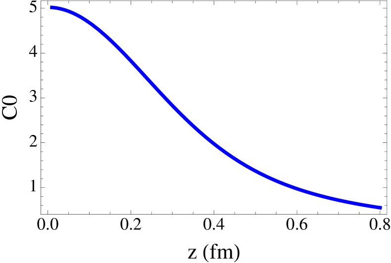
Figure 1: The function C0(z)subscript𝐶0𝑧C_{0}(z) for the selected parameters.
Refer to caption
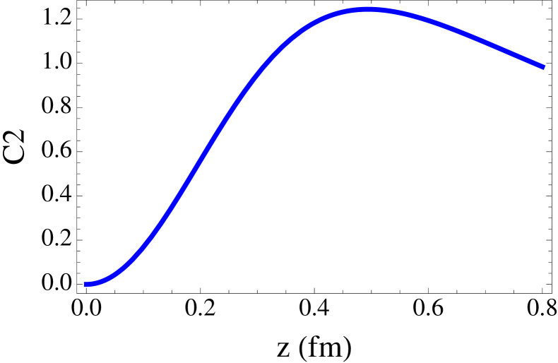
Figure 2: The function C2(z)subscript𝐶2𝑧C_{2}(z) for the selected parameters.

We now evaluate the average energy density and its fluctuations for a choice of the parameters that is motivated by the initial conditions at which thermal QCD matter is formed in heavy ion collisions at RHIC and LHC:

Qs2superscriptsubscript𝑄𝑠2\displaystyle Q_{s}^{2} =\displaystyle= (g2μ)2=2GeV2;superscriptsuperscript𝑔2𝜇22superscriptGeV2\displaystyle(g^{2}\mu)^{2}=2~{}{\rm GeV}^{2};
g2(μ2)superscript𝑔2superscript𝜇2\displaystyle g^{2}(\mu^{2}) =\displaystyle= 3.785;3.785\displaystyle 3.785;
g2(1/x2)superscript𝑔21superscript𝑥2\displaystyle g^{2}(1/x^{2}) =\displaystyle= 16π29ln(1/(Λ2x2)).16superscript𝜋291superscriptΛ2superscript𝑥2\displaystyle\frac{16\pi^{2}}{9\ln(1/(\Lambda^{2}x^{2}))}. (45)

Note that the result is independent of the value of ΛΛ\Lambda. The functions C0(z)subscript𝐶0𝑧C_{0}(z) and C2(z)subscript𝐶2𝑧C_{2}(z) are shown in Figs. 1 and 2 for these parameter values.

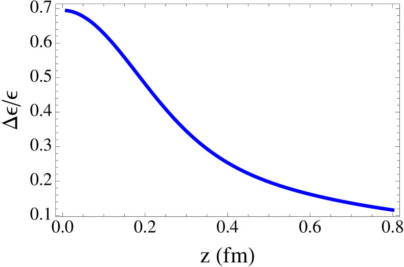
For these parameters, the initial value of the deposited energy density is ε0240GeV/fm3subscript𝜀0240GeVsuperscriptfm3\varepsilon_{0}\approx 240~{}{\rm GeV/fm}^{3}. This very large energy density quickly decreases due to the longitudinal expansion and reaches much smaller values by the time of thermalization. What matters for us is not the absolute value of the initial energy density, but the relative size and spatial correlation of its fluctuations, Δε(𝐱𝐲)/ε0Δ𝜀𝐱𝐲subscript𝜀0\Delta\varepsilon({\bf x}-{\bf y})/\varepsilon_{0}. This function is shown in Fig. 3 for the parameters listed above.
Refer to caption
Figure 3: The function Δε(z)/ε0Δ𝜀𝑧subscript𝜀0\Delta\varepsilon(z)/\varepsilon_{0} for the selected parameters.

As the figure shows, the fluctuations of the initial energy density are locally of similar magnitude as the energy density itself and fall over distances of the inverse saturation scale, here assumed as Qs10.14fmsuperscriptsubscript𝑄𝑠10.14fmQ_{s}^{-1}\approx 0.14~{}{\rm fm}. This result is in accord with the intuitive picture of the field configuration immediately after the collision in the color glass condensate model, as a bundle of longitudinally stretching random color flux tubes with characteristic transverse width 1/Qs1subscript𝑄𝑠1/Q_{s}.

V Summary

We have calculated the initial energy density fluctuations in high-energy heavy ion collisions within the Gaussian color glass condensate model. These turn out to be very large with a transverse profile determined by the saturation scale Qssubscript𝑄𝑠Q_{s}. A finite result is only obtained when the “triumvirate” running coupling is used, giving additional support to the correctness of Eq. (13). The fluctuation probabilities thus derived can serve as input for any calculation aiming at the investigation of early fluctuations, in particular for calculations which study the fate of such fluctuations during thermalization. For example, it is possible to investigate the problem of event-by-event fluctuations in heavy ion collisions within the AdS/CFT paradigm using methods similar to those employed in string .

Acknowledgments: This work was supported in part by the Office of Science of the U.S. Department of Energy (DE-FG02-05ER41367) and the BMBF (06 RY9191). We thank U. Heinz, J. Liu, Z. Qiu, and C. Shen for pointing out several typographical and numerical errors in an earlier version of this manuscript, and R. Venugopalan and H. Weigert for clarifying the Gaussian approximation in the color glass condensate model.

References

  • (1) B. Alver et al. [PHOBOS Collaboration], Phys. Rev. Lett.  104, 142301 (2010).
  • (2) P. Sorensen [STAR Collaboration], J. Phys. G G35, 104102 (2008).
  • (3) ALICE Collaboration, Phys. Rev. Lett.  107, 032301 (2011).
  • (4) A. Adare et al. [PHENIX Collaboration], arXiv:1105.3928 [nucl-ex].
  • (5) J. J. Jia [ATLAS Collaboration], arXiv:1107.1468 [nucl-ex].
  • (6) P. Sorensen [STAR Collaboration], arXiv:1110.0737 [nucl-ex].
  • (7) E. Appelt [CMS Collaboration], arXiv:1110.1026 [nucl-ex].
  • (8) M. Miller, R. Snellings, arXiv:nucl-ex/0312008.
  • (9) W. Broniowski, P. Bozek, M. Rybczynski, Phys. Rev.  C76, 054905 (2007).
  • (10) R. P. G. Andrade, F. Grassi, Y. Hama, T. Kodama, W. L. Qian, Phys. Rev. Lett.  101, 112301 (2008).
  • (11) E. Shuryak, Phys. Rev.  C80, 054908 (2009).
  • (12) B. Alver, G. Roland, Phys. Rev.  C81, 054905 (2010).
  • (13) H. Petersen, G. -Y. Qin, S. A. Bass, B. Müller, Phys. Rev.  C82, 041901 (2010).
  • (14) B. H. Alver, C. Gombeaud, M. Luzum, J. -Y. Ollitrault, Phys. Rev.  C82, 034913 (2010).
  • (15) P. Staig, E. Shuryak, arXiv:1106.3243 [hep-ph]; Phys. Rev.  C84, 034908 (2011); Phys. Rev.  C84, 044912 (2011).
  • (16) H. Holopainen, H. Niemi, K. J. Eskola, Phys. Rev.  C83, 034901 (2011).
  • (17) G. -Y. Qin, H. Petersen, S. A. Bass, B. Müller, Phys. Rev.  C82, 064903 (2010).
  • (18) B. Schenke, S. Jeon, C. Gale, Phys. Rev. Lett.  106, 042301 (2011).
  • (19) Z. Qiu, U. W. Heinz, Phys. Rev.  C84, 024911 (2011).
  • (20) R. S. Bhalerao, M. Luzum, J. -Y. Ollitrault, Phys. Rev.  C84, 034910 (2011); Phys. Rev.  C84, 054901 (2011).
  • (21) G. -Y. Qin, B. Müller, arXiv:1109.5961 [hep-ph].
  • (22) R. D. de Souza, J. Takahashi, T. Kodama, P. Sorensen, arXiv:1110.5698 [hep-ph].
  • (23) H. -J. Drescher, Y. Nara, Phys. Rev.  C75, 034905 (2007); Phys. Rev.  C76, 041903 (2007).
  • (24) L. D. McLerran and R. Venugopalan, Phys. Rev. D 49, 2233 (1994).
  • (25) L. D. McLerran, R. Venugopalan, Phys. Rev.  D49, 3352 (1994).
  • (26) A. H. Mueller, Nucl. Phys. B 558, 285 (1999).
  • (27) J. Jalilian-Marian, A. Kovner, A. Leonidov and H. Weigert, Phys. Rev. D 59, 014014 (1999).
  • (28) Y. V. Kovchegov, Phys. Rev. D 54, 5463 (1996);
  • (29) T. Lappi, Phys. Lett. B 643, 11 (2006).
  • (30) Y. V. Kovchegov and H. Weigert, Nucl. Phys.  A807, 158 (2008).
  • (31) Y. V. Kovchegov, H. Weigert, Nucl. Phys.  A789, 260 (2007).
  • (32) I. S. Gradshteyn and I. M. Ryzhik, Table of Integrals, Series and Products, Academic Press, Elsevier, 2007.
  • (33) V. Balasubramanian, et al., Phys. Rev. Lett.  106, 191601 (2011); Phys. Rev.  D84, 026010 (2011).
  • (34) C. Marquet and H. Weigert, Nucl. Phys. A 843, 68 (2010).