A simple energy loss model and its applications for silicon detectors

Ferenc Siklér sikler@rmki.kfki.hu KFKI Research Institute for Particle and Nuclear Physics, Budapest, Hungary
CERN, Geneva, Switzerland
Abstract

The energy loss of charged particles in silicon can be approximated by a simple analytical model. With help of measured charge deposits in individual channels of hit clusters their position and energy can be estimated. Deposits below threshold and saturated values are treated properly, resulting in a wider dynamic range. The proposed method gives improvements on both hit position and energy residuals. The model is successfully applied to track differential energy loss estimation and to detector gain calibration tasks.

keywords:
Energy loss , Silicon
PACS:
29.40.Gx , 29.85.-c , 34.50.Bw

1 Introduction

The identification of charged particles is essential in several fields of particle and nuclear physics: particle spectra, correlations, selection of daughters of resonance decays and for reducing the background of rare physics processes [1, 2]. Silicon detectors can be employed for identification by proper use of energy deposit measurements along the trajectory of the particle. The aim of this study is to provide a simple method to evaluate energy deposits and other derived quantities for a wide range of particle momenta (βγ=p/m=0.5610.0𝛽𝛾𝑝𝑚0.5610.0\beta\gamma=p/m=0.56-10.0) and detector thickness, based on the precise knowledge of the known underlying physics processes.

This article is organized as follows: the model is motivated and discussed in detail in Sec. 2. Among the various applications we will deal with the estimation of hit position (Sec. 3), hit energy deposit (Sec. 4), differential energy loss for tracks (Sec. 5), as well as detector gain calibration for tracks (Sec. 6). This work ends with conclusions.

105superscript10510^{-5}104superscript10410^{-4}103superscript10310^{-3}102superscript10210^{-2}101superscript10110^{-1}100superscript10010^{0}050100150200

p(y|l)𝑝conditional𝑦𝑙p(y|l)

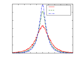
y𝑦y[keV]βγ=1.00𝛽𝛾1.00\beta\gamma=1.00Refer to captionl=20𝑙20l=~{}20μ𝜇\muml=50𝑙50l=~{}50μ𝜇\muml=100𝑙100l=100μ𝜇\muml=200𝑙200l=200μ𝜇\mum
Figure 1: Probability density functions for particles with βγ=1.00𝛽𝛾1.00\beta\gamma=1.00, at given path lengths of 20, 50, 100 and 200 μ𝜇\mum.

2 Simple energy loss model

When a charged particle traverses material it loses energy in several discrete steps, dominantly by resonance excitations (δ𝛿\delta-function) and Coulomb excitations (truncated 1/E21superscript𝐸21/E^{2} term). This latter is the reason for the long tail observed in energy deposit distributions. It is generally difficult to describe the process with a simple function. The most probable energy loss ΔΔ\Delta, and the full width of the energy loss distribution at half maximum ΓΔsubscriptΓΔ\Gamma_{\Delta} [3] can be approximated by

ΔΔ\displaystyle\Delta =ξ[log2mc2β2γ2ξI2+0.2000β2δ]absent𝜉delimited-[]2𝑚superscript𝑐2superscript𝛽2superscript𝛾2𝜉superscript𝐼20.2000superscript𝛽2𝛿\displaystyle=\xi\left[\log\frac{2mc^{2}\beta^{2}\gamma^{2}\xi}{I^{2}}+0.2000-\beta^{2}-\delta\right] (1)
ΓΔsubscriptΓΔ\displaystyle\Gamma_{\Delta} =4.018ξabsent4.018𝜉\displaystyle=4.018\xi
105superscript10510^{-5}104superscript10410^{-4}103superscript10310^{-3}102superscript10210^{-2}101superscript10110^{-1}100superscript10010^{0}0200400600800100012001400

fy(l)subscript𝑓𝑦𝑙f_{y}(l)

l𝑙l[μ𝜇\mum]βγ=𝛽𝛾absent\beta\gamma=3.16105superscript10510^{-5}104superscript10410^{-4}103superscript10310^{-3}102superscript10210^{-2}101superscript10110^{-1}100superscript10010^{0}0200400600800100012001400

fy(l)subscript𝑓𝑦𝑙f_{y}(l)

l𝑙l[μ𝜇\mum]105superscript10510^{-5}104superscript10410^{-4}103superscript10310^{-3}102superscript10210^{-2}101superscript10110^{-1}100superscript10010^{0}0200400600800100012001400

fy(l)subscript𝑓𝑦𝑙f_{y}(l)

l𝑙l[μ𝜇\mum]105superscript10510^{-5}104superscript10410^{-4}103superscript10310^{-3}102superscript10210^{-2}101superscript10110^{-1}100superscript10010^{0}0200400600800100012001400

fy(l)subscript𝑓𝑦𝑙f_{y}(l)

l𝑙l[μ𝜇\mum]Refer to caption
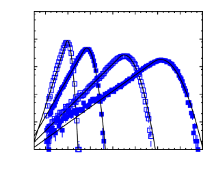
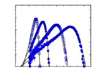
Figure 2: Fits of the conditional probability density fy(l)subscript𝑓𝑦𝑙f_{y}(l) as function of the path length l𝑙l for particles with βγ=3.16𝛽𝛾3.16\beta\gamma=3.16 (see Eq.(2)). The simulated values (points) and the fitted curves (lines) corresponding to y=50,100,200𝑦50100200y=50,100,200 and 300300300 keV are shown, from left to right.

where

ξ=K2z2ZAρlβ2𝜉𝐾2superscript𝑧2𝑍𝐴𝜌𝑙superscript𝛽2\xi=\frac{K}{2}z^{2}\frac{Z}{A}\rho\frac{l}{\beta^{2}}

is the Landau parameter; K=4πNAre2mec2=0.307075MeVcm2/mol𝐾4𝜋subscript𝑁𝐴superscriptsubscript𝑟𝑒2subscript𝑚𝑒superscript𝑐20.307075MeVsuperscriptcm2molK=4\pi N_{A}r_{e}^{2}m_{e}c^{2}=0.307~{}075~{}\mathrm{MeV~{}cm^{2}/mol}; Z𝑍Z, A𝐴A, ρ𝜌\rho and l𝑙l are the mass number, atomic number, density and thickness of the material, respectively; and δ𝛿\delta is the density correction [4].

The probability of an excitation, energy deposit, along the path of the incoming particle is a function of βγ=p/m𝛽𝛾𝑝𝑚\beta\gamma=p/m of the particle and depends on properties of the traversed material. The conditional probability density p(y|l)𝑝conditional𝑦𝑙p(y|l), deposit y𝑦y along a given path length l𝑙l, can be built using the above mentioned elementary excitations combined with an exponential occurrence model. The details of the microscopical simulation for silicon can be found in Refs. [3], [5] and [6]. The result of these recursive convolutions is a smooth function (Fig. 1).
00.20.40.60.810200400600800

y/lP𝑦subscript𝑙𝑃y/l_{P}[keV/μ𝜇\mum]

lPsubscript𝑙𝑃l_{P}[μ𝜇\mum]Refer to captionβγ=0.56𝛽𝛾0.56\beta\gamma=0.56βγ=1.00𝛽𝛾1.00\beta\gamma=1.00βγ=3.16𝛽𝛾3.16\beta\gamma=3.16βγ=10.0𝛽𝛾10.0\beta\gamma=10.0
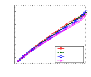
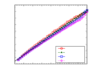
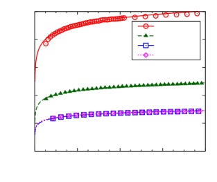
Figure 3: Relationship between the measured deposited energy y𝑦y and the position of the path length peak lpsubscript𝑙𝑝l_{p}, shown together with fits using Eq. 3.
051015202530354045050100150200250300350400

σlsubscript𝜎𝑙\sigma_{l}[μ𝜇\mum]

y𝑦y[keV]Refer to captionβγ=0.56𝛽𝛾0.56\beta\gamma=0.56βγ=1.00𝛽𝛾1.00\beta\gamma=1.00βγ=3.16𝛽𝛾3.16\beta\gamma=3.16βγ=10.0𝛽𝛾10.0\beta\gamma=10.0
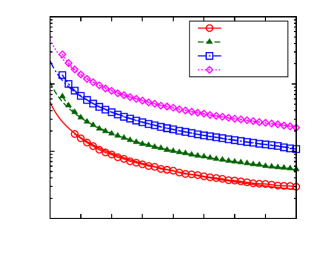
Figure 4: Relationship between the measured deposited energy y𝑦y and the standard deviation σlsubscript𝜎𝑙\sigma_{l} of l𝑙l distribution.

In the experiment the deposit values y𝑦y are measured. For a fixed y𝑦y the conditional probability can be regarded as function of l𝑙l, thus p(y|l)fy(l)𝑝conditional𝑦𝑙subscript𝑓𝑦𝑙p(y|l)\equiv f_{y}(l). Values of fy(l)subscript𝑓𝑦𝑙f_{y}(l) for particles with βγ=3.16𝛽𝛾3.16\beta\gamma=3.16 are plotted in Fig. 2, where the values corresponding to y=50,100,200𝑦50100200y=50,100,200 and 300300300 keV are shown. Other βγ𝛽𝛾\beta\gamma settings show very similar behavior (βγ=0.56,1.00𝛽𝛾0.561.00\beta\gamma=0.56,1.00 and 10.010.010.0, not plotted). Apart from a multiplicative factor, they are well approximated by a combination of simple functions, exponential and Gaussian:

fy(l){exp(ν(llP)σl+ν22),if l<lexp((llP)22σl2),if llproportional-tosubscript𝑓𝑦𝑙cases𝜈𝑙subscript𝑙𝑃subscript𝜎𝑙superscript𝜈22if l<lsuperscript𝑙subscript𝑙𝑃22superscriptsubscript𝜎𝑙2if llf_{y}(l)\propto\begin{cases}\exp\left(\frac{\nu(l-l_{P})}{\sigma_{l}}+\frac{\nu^{2}}{2}\right),&\text{if $l<l^{*}$}\\ \exp\left(-\frac{(l-l_{P})^{2}}{2\sigma_{l}^{2}}\right),&\text{if $l\geq l^{*}$}\end{cases} (2)

where the limit is

l=lPνσl.superscript𝑙subscript𝑙𝑃𝜈subscript𝜎𝑙l^{*}=l_{P}-\nu\sigma_{l}.

The peak position lPsubscript𝑙𝑃l_{P} and standard deviation σlsubscript𝜎𝑙\sigma_{l} are both functions of y𝑦y and βγ𝛽𝛾\beta\gamma, ν0.65𝜈0.65\nu\approx 0.65 is constant. Note that fysubscript𝑓𝑦f_{y} is constructed such that the value and the derivative are continuous at the limit lsuperscript𝑙l^{*}. The peak position lPsubscript𝑙𝑃l_{P} is roughly proportional to the deposit y𝑦y, their relationship can be approximated as

yεlp[1+0.08log(lP/l0)]𝑦𝜀subscript𝑙𝑝delimited-[]10.08subscript𝑙𝑃subscript𝑙0y\approx\varepsilon l_{p}\left[1+0.08\log(l_{P}/l_{0})\right] (3)

where l0subscript𝑙0l_{0} is some reference path length (Fig. 3). In this work l0=subscript𝑙0absentl_{0}= 300 μ𝜇\mum was chosen. At the same time σlsubscript𝜎𝑙\sigma_{l} has an approximate first order polynomial dependence on y𝑦y (Fig. 4).

As it was shown above, some interesting connections between the deposit and path length can be observed, for wide range of βγ𝛽𝛾\beta\gamma values. Unfortunately the dependence on βγ𝛽𝛾\beta\gamma, and l𝑙l, is still present. In the following (Sec. 2.1) we will show how that can be suppressed or even eliminated.

2.1 Most probable differential energy loss

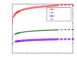
The path length dependence of the most probable energy loss ΔΔ\Delta (Fig. 5) has a form that is very similar to Eq. (3). The dependence can be approximated by

Δ(l)εl[1+alog(l/l0)]Δ𝑙𝜀𝑙delimited-[]1𝑎𝑙subscript𝑙0\Delta(l)\approx\varepsilon l\left[1+a\log(l/l_{0})\right] (4)

where ε𝜀\varepsilon is the most probable differential energy loss along a reference length l0subscript𝑙0l_{0}, hence ε=Δ(l0)/l0𝜀Δsubscript𝑙0subscript𝑙0\varepsilon=\Delta(l_{0})/l_{0}. For the relevant βγ𝛽𝛾\beta\gamma region studied in this paper a0.07𝑎0.07a\approx 0.07, to a good approximation.111Based on Eq. 1, with some approximations, the expected magnitude of a𝑎a would be 1/log(2mec2Kz2Z/Aρ/I2)0.06412subscript𝑚𝑒superscript𝑐2𝐾superscript𝑧2𝑍𝐴𝜌superscript𝐼20.0641/\log(2m_{e}c^{2}Kz^{2}\cdot Z/A\cdot\rho/I^{2})\approx 0.064. For some applications, such as hit position estimation, the assumption of linearity may be enough (see Eq. (17) later).
00.20.40.60.810200400600800

Δ/lΔ𝑙\Delta/l[keV/μ𝜇\mum]

l𝑙l[μ𝜇\mum]Refer to captionβγ=0.56𝛽𝛾0.56\beta\gamma=0.56βγ=1.00𝛽𝛾1.00\beta\gamma=1.00βγ=3.16𝛽𝛾3.16\beta\gamma=3.16βγ=10.0𝛽𝛾10.0\beta\gamma=10.0
Figure 5: Relationship between the most probable energy deposit ΔΔ\Delta and the path length l𝑙l, shown together with fits using Eq. 4.

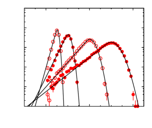
Hence it is worthwhile to check whether the dependence on βγ𝛽𝛾\beta\gamma and l𝑙l can be suppressed by taking the most probable deposit ΔΔ\Delta as variable of the conditional probability. Values of p(y|Δ)fy(Δ)𝑝conditional𝑦Δsubscript𝑓𝑦Δp(y|\Delta)\equiv f_{y}(\Delta) for particles with βγ=0.56,1.00,3.16𝛽𝛾0.561.003.16\beta\gamma=0.56,1.00,3.16 and 10.010.010.0 are plotted in Fig. 6, where the values corresponding to y=50,100,200𝑦50100200y=50,100,200, and 300300300 keV are shown. The distributions for a given y𝑦y value are remarkably similar for all βγ𝛽𝛾\beta\gamma values.

105superscript10510^{-5}104superscript10410^{-4}103superscript10310^{-3}102superscript10210^{-2}101superscript10110^{-1}100superscript10010^{0}0200400

fy(Δ)subscript𝑓𝑦Δf_{y}(\Delta)

ΔΔ\Delta[keV]βγ=𝛽𝛾absent\beta\gamma=0.56105superscript10510^{-5}104superscript10410^{-4}103superscript10310^{-3}102superscript10210^{-2}101superscript10110^{-1}100superscript10010^{0}0200400

fy(Δ)subscript𝑓𝑦Δf_{y}(\Delta)

ΔΔ\Delta[keV]105superscript10510^{-5}104superscript10410^{-4}103superscript10310^{-3}102superscript10210^{-2}101superscript10110^{-1}100superscript10010^{0}0200400

fy(Δ)subscript𝑓𝑦Δf_{y}(\Delta)

ΔΔ\Delta[keV]105superscript10510^{-5}104superscript10410^{-4}103superscript10310^{-3}102superscript10210^{-2}101superscript10110^{-1}100superscript10010^{0}0200400

fy(Δ)subscript𝑓𝑦Δf_{y}(\Delta)

ΔΔ\Delta[keV]Refer to caption
105superscript10510^{-5}104superscript10410^{-4}103superscript10310^{-3}102superscript10210^{-2}101superscript10110^{-1}100superscript10010^{0}0200400

fy(Δ)subscript𝑓𝑦Δf_{y}(\Delta)

ΔΔ\Delta[keV]βγ=𝛽𝛾absent\beta\gamma=1.00105superscript10510^{-5}104superscript10410^{-4}103superscript10310^{-3}102superscript10210^{-2}101superscript10110^{-1}100superscript10010^{0}0200400

fy(Δ)subscript𝑓𝑦Δf_{y}(\Delta)

ΔΔ\Delta[keV]105superscript10510^{-5}104superscript10410^{-4}103superscript10310^{-3}102superscript10210^{-2}101superscript10110^{-1}100superscript10010^{0}0200400

fy(Δ)subscript𝑓𝑦Δf_{y}(\Delta)

ΔΔ\Delta[keV]105superscript10510^{-5}104superscript10410^{-4}103superscript10310^{-3}102superscript10210^{-2}101superscript10110^{-1}100superscript10010^{0}0200400

fy(Δ)subscript𝑓𝑦Δf_{y}(\Delta)

ΔΔ\Delta[keV]Refer to caption
105superscript10510^{-5}104superscript10410^{-4}103superscript10310^{-3}102superscript10210^{-2}101superscript10110^{-1}100superscript10010^{0}0200400

fy(Δ)subscript𝑓𝑦Δf_{y}(\Delta)

ΔΔ\Delta[keV]βγ=𝛽𝛾absent\beta\gamma=3.16105superscript10510^{-5}104superscript10410^{-4}103superscript10310^{-3}102superscript10210^{-2}101superscript10110^{-1}100superscript10010^{0}0200400

fy(Δ)subscript𝑓𝑦Δf_{y}(\Delta)

ΔΔ\Delta[keV]105superscript10510^{-5}104superscript10410^{-4}103superscript10310^{-3}102superscript10210^{-2}101superscript10110^{-1}100superscript10010^{0}0200400

fy(Δ)subscript𝑓𝑦Δf_{y}(\Delta)

ΔΔ\Delta[keV]105superscript10510^{-5}104superscript10410^{-4}103superscript10310^{-3}102superscript10210^{-2}101superscript10110^{-1}100superscript10010^{0}0200400

fy(Δ)subscript𝑓𝑦Δf_{y}(\Delta)

ΔΔ\Delta[keV]Refer to caption
105superscript10510^{-5}104superscript10410^{-4}103superscript10310^{-3}102superscript10210^{-2}101superscript10110^{-1}100superscript10010^{0}0200400

fy(Δ)subscript𝑓𝑦Δf_{y}(\Delta)

ΔΔ\Delta[keV]βγ=𝛽𝛾absent\beta\gamma=10.00105superscript10510^{-5}104superscript10410^{-4}103superscript10310^{-3}102superscript10210^{-2}101superscript10110^{-1}100superscript10010^{0}0200400

fy(Δ)subscript𝑓𝑦Δf_{y}(\Delta)

ΔΔ\Delta[keV]105superscript10510^{-5}104superscript10410^{-4}103superscript10310^{-3}102superscript10210^{-2}101superscript10110^{-1}100superscript10010^{0}0200400

fy(Δ)subscript𝑓𝑦Δf_{y}(\Delta)

ΔΔ\Delta[keV]105superscript10510^{-5}104superscript10410^{-4}103superscript10310^{-3}102superscript10210^{-2}101superscript10110^{-1}100superscript10010^{0}0200400

fy(Δ)subscript𝑓𝑦Δf_{y}(\Delta)

ΔΔ\Delta[keV]Refer to caption
Figure 6: Fits of the conditional probability density fy(Δ)subscript𝑓𝑦Δf_{y}(\Delta) as function of the most probable energy loss ΔΔ\Delta for particles with βγ=0.56𝛽𝛾0.56\beta\gamma=0.56, 1.001.001.00, 3.163.163.16, and 10.010.010.0 (see Eq. (5)). The simulated values (points) and the fitted curves (lines) corresponding to y=50,100,200𝑦50100200y=50,100,200 and 300300300 keV are shown, from left to right.
051015202530354045050100150200250300350400

σΔsubscript𝜎Δ\sigma_{\Delta}[keV]

y𝑦y[keV]σ02.1subscript𝜎02.1\sigma_{0}\approx 2.1keVb0.094𝑏0.094b\approx 0.094Refer to captionβγ=0.56𝛽𝛾0.56\beta\gamma=0.56βγ=1.00𝛽𝛾1.00\beta\gamma=1.00βγ=3.16𝛽𝛾3.16\beta\gamma=3.16βγ=10.0𝛽𝛾10.0\beta\gamma=10.0
103superscript10310^{-3}102superscript10210^{-2}101superscript10110^{-1}100superscript10010^{0}050100150200250300350400

C(y)

y [keV]103superscript10310^{-3}102superscript10210^{-2}101superscript10110^{-1}100superscript10010^{0}050100150200250300350400

C(y)

y [keV]103superscript10310^{-3}102superscript10210^{-2}101superscript10110^{-1}100superscript10010^{0}050100150200250300350400

C(y)

y [keV]103superscript10310^{-3}102superscript10210^{-2}101superscript10110^{-1}100superscript10010^{0}050100150200250300350400

C(y)

y [keV]103superscript10310^{-3}102superscript10210^{-2}101superscript10110^{-1}100superscript10010^{0}050100150200250300350400

C(y)

y [keV]Refer to captionβγ=𝛽𝛾absent\beta\gamma=0.56βγ=𝛽𝛾absent\beta\gamma=1.00βγ=𝛽𝛾absent\beta\gamma=3.16βγ=𝛽𝛾absent\beta\gamma=10.0
Figure 7: Left: Relationship between the measured deposited energy y𝑦y and the standard deviation σΔsubscript𝜎Δ\sigma_{\Delta} of ΔΔ\Delta distribution. Right: The measured value of C(y)𝐶𝑦C(y) for particles with βγ=0.56𝛽𝛾0.56\beta\gamma=0.56, 1.001.001.00, 3.163.163.16, and 10.010.010.0. The points and curves are successively multiplied by factors of 2 for clarity. Note that the plotted function 1/σΔ(y)1subscript𝜎Δ𝑦1/\sigma_{\Delta}(y) is the same in all cases except for the multiplicative factor mentioned before.

The conditional probability density for a given y𝑦y, as a function of ΔΔ\Delta can be described as

fy(Δ)C(y){exp(ν(Δy)σΔ+ν22),if Δ<Δexp((Δy)22σΔ2),if ΔΔsubscript𝑓𝑦Δ𝐶𝑦cases𝜈Δ𝑦subscript𝜎Δsuperscript𝜈22if Δ<ΔsuperscriptΔ𝑦22superscriptsubscript𝜎Δ2if ΔΔf_{y}(\Delta)\approx C(y)\cdot\begin{cases}\exp\left(\frac{\nu(\Delta-y)}{\sigma_{\Delta}}+\frac{\nu^{2}}{2}\right),&\text{if $\Delta<\Delta^{*}$}\\ \exp\left(-\frac{(\Delta-y)^{2}}{2\sigma_{\Delta}^{2}}\right),&\text{if $\Delta\geq\Delta^{*}$}\end{cases} (5)

where C(y)𝐶𝑦C(y) is a universal function of y𝑦y. Note that fysubscript𝑓𝑦f_{y} is constructed such that the value and the derivative are continuous at the limit ΔsuperscriptΔ\Delta^{*} that is given by

Δ(y)=yνσΔ(y)superscriptΔ𝑦𝑦𝜈subscript𝜎Δ𝑦\Delta^{*}(y)=y-\nu\sigma_{\Delta}(y) (6)

where ν0.65𝜈0.65\nu\approx 0.65 is constant. Fig. 7-left shows that σΔsubscript𝜎Δ\sigma_{\Delta} is a first order polynomial of y𝑦y, practically independent of βγ𝛽𝛾\beta\gamma, in the form

σΔ(y)=σ0+bysubscript𝜎Δ𝑦subscript𝜎0𝑏𝑦\sigma_{\Delta}(y)=\sigma_{0}+by (7)

where σ0subscript𝜎0absent\sigma_{0}\approx 2 keV, b0.095𝑏0.095b\approx 0.095. According to Fig. 7-right the y𝑦y dependent coefficient of Eq. (5) is very well approximated as

C(y)𝐶𝑦\displaystyle C(y) 1/σΔ(y).proportional-toabsent1subscript𝜎Δ𝑦\displaystyle\propto 1/\sigma_{\Delta}(y). (8)

The parameters of the above detailed energy loss model and their short explanations are listed in Table 1. Note that these four numbers are the only parameters of the description. Usually the detector and readout noise can be neglected. If this is not the case the term σΔ2superscriptsubscript𝜎Δ2\sigma_{\Delta}^{2} in Eq. (5) and (8) should be replaced by σD2+σn2superscriptsubscript𝜎𝐷2superscriptsubscript𝜎𝑛2\sigma_{D}^{2}+\sigma_{n}^{2} where σnsubscript𝜎𝑛\sigma_{n} is the standard deviation of the Gaussian noise.

Table 1: Parameters of the energy loss model.
ν𝜈\nu 0.65 Gaussian vs exponential [σΔ(y)subscript𝜎Δ𝑦\sigma_{\Delta}(y)]
a𝑎a 0.07 coefficient of log term in Δ(l)Δ𝑙\Delta(l)
σ0subscript𝜎0\sigma_{0} 2 keV constant term of σΔ(y)subscript𝜎Δ𝑦\sigma_{\Delta}(y)
b𝑏b 0.095 linear coefficient of σΔ(y)subscript𝜎Δ𝑦\sigma_{\Delta}(y)

2.2 Left truncation and right censoring

During readout the deposited energy is converted to measured ADC values through several steps: primary and secondary electron-hole pairs, current signals, front-end electronics, digitization [7]. In this study we assume that the response of the detector system is linear in the threshold-to-censoring region. Signals below threshold are truncated, since they produce no output. Signals above a certain level are censored, hence only the fact that the deposit was above that level is known. Note that the censoring level does not necessarily coincides with the saturation level of the readout electronics: the former is simply chosen as the limit of linearity.

If the measured value y𝑦y is below or above a limit t𝑡t, the corresponding values can be calculated by integration

fy<t(Δ)subscript𝑓𝑦𝑡Δ\displaystyle f_{y<t}(\Delta) =tfy(Δ)dy,absentsuperscriptsubscript𝑡subscript𝑓𝑦Δdifferential-d𝑦\displaystyle=\int_{-\infty}^{t}f_{y}(\Delta)\mathrm{d}y, fy>t(Δ)subscript𝑓𝑦𝑡Δ\displaystyle f_{y>t}(\Delta) =tfy(Δ)dy.absentsuperscriptsubscript𝑡subscript𝑓𝑦Δdifferential-d𝑦\displaystyle=\int_{t}^{\infty}f_{y}(\Delta)\mathrm{d}y.

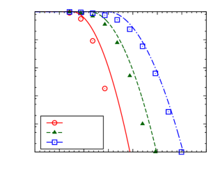
Note that since σΔsubscript𝜎Δ\sigma_{\Delta} is a function of y𝑦y, the integrals are difficult to perform. The simulated values with several truncation thresholds and censoring levels are shown in Fig. 8. They are well approximated by the following functional forms:

fy<t(Δ)subscript𝑓𝑦𝑡Δ\displaystyle f_{y<t}(\Delta) ={1,if Δ<tσΔexp[12(ΔtσΔ+1)2],if ΔtσΔabsentcases1if Δ<tσΔ12superscriptΔ𝑡subscript𝜎Δ12if ΔtσΔ\displaystyle=\begin{cases}1,&\text{if $\Delta<t-\sigma_{\Delta}$}\\ \exp\left[-\frac{1}{2}\left(\frac{\Delta-t}{\sigma_{\Delta}}+1\right)^{2}\right],&\text{if $\Delta\geq t-\sigma_{\Delta}$}\end{cases} (9)
fy>t(Δ)subscript𝑓𝑦𝑡Δ\displaystyle f_{y>t}(\Delta) ={exp[12(ΔtσΔ1)],if Δ<t+σΔ1,if Δt+σΔ.absentcases12Δ𝑡subscript𝜎Δ1if Δ<t+σΔ1if Δt+σΔ\displaystyle=\begin{cases}\exp\left[\frac{1}{2}\left(\frac{\Delta-t}{\sigma_{\Delta}}-1\right)\right],&\;\;\;\;\text{if $\Delta<t+\sigma_{\Delta}$}\\ 1,&\;\;\;\;\text{if $\Delta\geq t+\sigma_{\Delta}$}.\end{cases} (10)
105superscript10510^{-5}104superscript10410^{-4}103superscript10310^{-3}102superscript10210^{-2}101superscript10110^{-1}100superscript10010^{0}-5051015202530

fy<t(Δ)subscript𝑓𝑦𝑡Δf_{y<t}(\Delta)

ΔΔ\Delta[keV]Refer to captionfy<5keVsubscript𝑓𝑦5keVf_{y<5~{}\mathrm{keV}}fy<9keVsubscript𝑓𝑦9keVf_{y<9~{}\mathrm{keV}}fy<13keVsubscript𝑓𝑦13keVf_{y<13~{}\mathrm{keV}}
105superscript10510^{-5}104superscript10410^{-4}103superscript10310^{-3}102superscript10210^{-2}101superscript10110^{-1}100superscript10010^{0}050100150200

fy>t(Δ)subscript𝑓𝑦𝑡Δf_{y>t}(\Delta)

ΔΔ\Delta[keV]Refer to captionfy>80keVsubscript𝑓𝑦80keVf_{y>80~{}\mathrm{keV}}fy>135keVsubscript𝑓𝑦135keVf_{y>135~{}\mathrm{keV}}fy>180keVsubscript𝑓𝑦180keVf_{y>180~{}\mathrm{keV}}
Figure 8: Fits of the conditional probability fyt(Δ)subscript𝑓less-than-or-greater-than𝑦𝑡Δf_{y\lessgtr t}(\Delta) for measurements below threshold (left) and above censoring level (right) as function of ΔΔ\Delta, in case of several limiting values. Examples thresholds are 5, 9 and 13 keV, while censoring levels are at 80, 135 and 180 keV. The simulated values (points) are shown for particles with βγ=3.16𝛽𝛾3.16\beta\gamma=3.16, together with the fitted curves (lines, from Eqs. (9) and (10)).

2.3 Log-likelihood minimization

In summary, for a given measured deposit y𝑦y the probability density will be a function of ΔΔ\Delta only. The measure of goodness can be obtained with help of the log-likelihood value as

χ2=2logf.superscript𝜒22𝑓\chi^{2}=-2\log f.

For a given channel, with measured (y𝑦y) or limited deposit values (t𝑡t), the corresponding χ2superscript𝜒2\chi^{2} can be derived from Eqs. (5)-(8) and (9)-(10) and they are shown below:

χy2(Δ)=2logσΔ(y)++{2ν(Δy)σΔ(y)ν2,if Δ<yνσΔ(y)(ΔyσΔ(y))2,if ΔyνσΔ(y)subscriptsuperscript𝜒2𝑦Δ2subscript𝜎Δ𝑦cases2𝜈Δ𝑦subscript𝜎Δ𝑦superscript𝜈2if Δ<yνσΔ(y)superscriptΔ𝑦subscript𝜎Δ𝑦2if ΔyνσΔ(y)\displaystyle\begin{split}\chi^{2}_{y}(\Delta)&=2\log\sigma_{\Delta}(y)+\\ &+\begin{cases}\frac{-2\nu(\Delta-y)}{\sigma_{\Delta}(y)}-\nu^{2},&\text{if $\Delta<y-\nu\sigma_{\Delta}(y)$}\\ \left(\frac{\Delta-y}{\sigma_{\Delta}(y)}\right)^{2},&\text{if $\Delta\geq y-\nu\sigma_{\Delta}(y)$}\end{cases}\end{split} (11)
χy<t2(Δ)subscriptsuperscript𝜒2𝑦𝑡Δ\displaystyle\chi^{2}_{y<t}(\Delta) ={0,if Δ<tσΔ(t)(ΔtσΔ(t)+1)2,if ΔtσΔ(t)absentcases0if Δ<tσΔ(t)superscriptΔ𝑡subscript𝜎Δ𝑡12if ΔtσΔ(t)\displaystyle=\begin{cases}0,&\;\,\text{if $\Delta<t-\sigma_{\Delta}(t)$}\\ \left(\frac{\Delta-t}{\sigma_{\Delta}(t)}+1\right)^{2},&\;\,\text{if $\Delta\geq t-\sigma_{\Delta}(t)$}\end{cases} (12)
χy>t2(Δ)subscriptsuperscript𝜒2𝑦𝑡Δ\displaystyle\chi^{2}_{y>t}(\Delta) ={ΔtσΔ(t)+1,if Δ<t+σΔ(t)0,if Δt+σΔ(t)absentcasesΔ𝑡subscript𝜎Δ𝑡1if Δ<t+σΔ(t)0if Δt+σΔ(t)\displaystyle=\begin{cases}-\frac{\Delta-t}{\sigma_{\Delta}(t)}+1,&\;\;\;\;\text{if $\Delta<t+\sigma_{\Delta}(t)$}\\ 0,&\;\;\;\;\text{if $\Delta\geq t+\sigma_{\Delta}(t)$}\end{cases} (13)

where σΔ(y)subscript𝜎Δ𝑦\sigma_{\Delta}(y) is given by Eq. (7). The terms on the right side contain only linear or positive definite quadratic functions of ΔΔ\Delta. We can estimate ε𝜀\varepsilon for single hits or for the whole particle trajectory by minimizing the sum of corresponding chi-square values.

The proposed model has several applications, such as

  • 1.

    for a given hit the estimation of position 𝑷𝑷{\boldsymbol{P}} and energy deposit via optimizing ε𝜀\varepsilon and the individual path lengths lisubscript𝑙𝑖l_{i} in the various sensitive units, channels, of the detector (Sec. 3 and 4).

  • 2.

    for a given trajectory the estimation of most probable differential energy loss via optimizing ε𝜀\varepsilon (Sec. 5).

  • 3.

    detector gain (cross-)calibration with tracks via the variation of the chip by chip gain, hence by modifying the y𝑦y values (Sec. 6).

2.4 Estimation of parameter errors

In case of normal approximations, the inverse of the observed, sample based, Fisher information \cal I can be used to estimate the covariance of the fitted parameters V𝑉V [8]:

jksubscript𝑗𝑘\displaystyle{\cal I}_{jk} =122iχi2ajak,absent12superscript2subscript𝑖superscriptsubscript𝜒𝑖2subscript𝑎𝑗subscript𝑎𝑘\displaystyle=\frac{1}{2}\frac{\partial^{2}\sum_{i}\chi_{i}^{2}}{\partial a_{j}\partial a_{k}}, V𝑉\displaystyle V 1absentsuperscript1\displaystyle\approx-{\cal I}^{-1}

where iχi2subscript𝑖superscriptsubscript𝜒𝑖2\sum_{i}\chi_{i}^{2} denotes the joint chi-square of hit channels or trajectory hits.

2.5 Generation of random deposits

If the expected shape of the distribution of the estimator has to be determined using Monte Carlo simulation, the generation of deposits should be fast but precise. The energy deposit distribution function

P(y|Δ)1σΔ(y){exp[(Δy)22σΔ(y)2],if y<Δ+νσΔ(y)exp[ν(Δy)σΔ(y)+ν22],if yΔ+νσΔ(y)proportional-to𝑃conditional𝑦Δ1subscript𝜎Δ𝑦casessuperscriptΔ𝑦22subscript𝜎Δsuperscript𝑦2if y<Δ+νσΔ(y)𝜈Δ𝑦subscript𝜎Δ𝑦superscript𝜈22if yΔ+νσΔ(y)P(y|\Delta)\propto\frac{1}{\sigma_{\Delta}(y)}\cdot\begin{cases}\exp\left[-\frac{(\Delta-y)^{2}}{2\sigma_{\Delta}(y)^{2}}\right],&\text{if $y<\Delta+\nu\sigma_{\Delta}(y)$}\\ \exp\left[\frac{\nu(\Delta-y)}{\sigma_{\Delta}(y)}+\frac{\nu^{2}}{2}\right],&\text{if $y\geq\Delta+\nu\sigma_{\Delta}(y)$}\end{cases}

does not have a closed antiderivative, hence a simple inverse transform sampling is not possible. Due to its long high energy tail the acceptance-rejection method is also highly ineffective.

Let us suppose that we have generated a random deposit y0subscript𝑦0y_{0} at a given Δ0subscriptΔ0\Delta_{0}. The value y0subscript𝑦0y_{0} can be simply transformed to get a proper random deposit y𝑦y for ΔΔ\Delta with a linear transformation as

yΔσΔ(Δ)=y0Δ0σΔ(Δ0).𝑦Δsubscript𝜎ΔΔsubscript𝑦0subscriptΔ0subscript𝜎ΔsubscriptΔ0\frac{y-\Delta}{\sigma_{\Delta}(\Delta)}=\frac{y_{0}-\Delta_{0}}{\sigma_{\Delta}(\Delta_{0})}.

The distribution of y𝑦y can be deduced from P(y0|Δ0)𝑃conditionalsubscript𝑦0subscriptΔ0P(y_{0}|\Delta_{0}) and it can be shown that it equals with P(y|Δ)𝑃conditional𝑦ΔP(y|\Delta). The key of the proof is the identity

σΔ(Δ0)σΔ(Δ)σΔ(y)σΔ(y0)=1.subscript𝜎ΔsubscriptΔ0subscript𝜎ΔΔsubscript𝜎Δ𝑦subscript𝜎Δsubscript𝑦01\frac{\sigma_{\Delta}(\Delta_{0})}{\sigma_{\Delta}(\Delta)}\frac{\sigma_{\Delta}(y)}{\sigma_{\Delta}(y_{0})}=1.

3 Estimation of hit position

During the passage of a charged particle through sensitive silicon volumes one or more channels (pixels or strips) are hit. The charges created in the adjacent channels are recorded (electrons or holes), they provide input for hit cluster recognition. Here the task is to estimate the position 𝑷𝑷{\boldsymbol{P}} of the hit, location of the trajectory in the central plane, using the measured deposits.

Throughout this paper it is required that the local direction of the trajectory, hence the vector of the projected passage 𝝀𝝀{\boldsymbol{\lambda}} (projected onto the surface layer by drift), is known (Fig. 9). In other words only the re-estimation of cluster parameters is attempted.

3.1 Standard estimation

The simplest way of hit position estimation (labeled as Weighted) is the weighted mean of channel positions 𝒑𝒊subscript𝒑𝒊{\boldsymbol{p_{i}}}, where weights are the corresponding energy deposits yisubscript𝑦𝑖y_{i}:

𝑷Weighted=iyi𝒑𝒊iyi.subscript𝑷Weightedsubscript𝑖subscript𝑦𝑖subscript𝒑𝒊subscript𝑖subscript𝑦𝑖\displaystyle{\boldsymbol{P}}_{\mathrm{Weighted}}=\frac{\sum_{i}y_{i}{\boldsymbol{p_{i}}}}{\sum_{i}y_{i}}.

Another widely used standard reconstruction technique (labeled as First-last) deals only with one dimensional clusters [9, 10]. This treatment is natural for strip detectors. For pixels the cluster is projected onto both directions (x𝑥x and y𝑦y) and the two projections are analyzed separately. Only the first and last, projected and summed, channels are used for position determination, because that choice reduces the sensitivity to fluctuations in energy deposition. If the energy would be lost steadily, the estimated projected hit position would be

𝑷Firstlast=𝒑𝑭+𝒑𝑳2+yLyF2(yL+yF)𝝀𝒆𝒇𝒇subscript𝑷Firstlastsubscript𝒑𝑭subscript𝒑𝑳2subscript𝑦𝐿subscript𝑦𝐹2subscript𝑦𝐿subscript𝑦𝐹subscript𝝀𝒆𝒇𝒇{\boldsymbol{P}}_{\mathrm{First-last}}=\frac{{\boldsymbol{p_{F}}}+{\boldsymbol{p_{L}}}}{2}+\frac{y_{L}-y_{F}}{2(y_{L}+y_{F})}{\boldsymbol{\lambda_{eff}}}

where the x𝑥x and y𝑦y components of 𝝀𝒆𝒇𝒇subscript𝝀𝒆𝒇𝒇{\boldsymbol{\lambda_{eff}}} are the sum of the path lengths in the two corresponding edge channels. The above formula can be further corrected for the drift direction if the silicon was placed in magnetic field.

Due to the use of projections, relevant informations corresponding to the shape of hit cluster and its deposits are lost. In this work a new method is presented which takes each individual channel of the cluster into account.

3.2 Estimation using the model

The passage of a charged particle through the silicon layer is given by the entry and exit points of its trajectory. Even in magnetic field or for very slow particles the passage is very well approximated by a straight line, the entry and exit points being on different sides of the layer. The deposited charge along the passage is projected onto the surface layer by drift, as result of electric and magnetic fields. The local direction of the particle at a silicon unit can be calculated using the parameters of the trajectory and the vector of the projected passage 𝝀𝝀{\boldsymbol{\lambda}} is known.

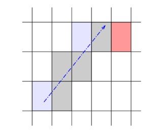
Refer to captionbelowthresh𝝀𝝀{\boldsymbol{\lambda}}2738443012belowthreshoutlier
Figure 9: Example cluster with measured deposits (rounded numbers in keV) and the the projected passage 𝝀𝝀{\boldsymbol{\lambda}} (arrow) at some stage of the minimization. The pixels below threshold are indicated with a lighter fill (below thresh.), while the outlier pixel has a darker fill than the others.

The following discussion deals with pixel silicon detectors, but it can be easily applied to strips by taking one of the pixel dimensions to very large values. During clustering neighboring pixels (those with common edge or vertex) are grouped to form a cluster, a reconstructed hit (Fig. 9). For the analysis of the corresponding cluster two types of pixels are of importance:

  • 1.

    A touched pixel is touched by the projected passage, regardless of its measured deposit. It can belong to the cluster (non-zero deposit) but it may be an empty pixel as well, if the deposited charge was below the threshold. The intersections of the projected passage and the edges of a pixel naturally give the projected path length inside that pixel.

  • 2.

    An outlier pixel is not crossed by the projected passage but it is a member of the cluster (non-zero deposit). In other words this pixel is an outlier, mostly left by a secondary particle, often δ𝛿\delta-electrons, created during the passage of the charged particle in the silicon. The projected passage does not have any section inside the pixel, but it is possible to construct a measure of the pixel-passage distance, a sort of negative path length (see Sec. 3.3). That notion is important in order to properly take into account the effect of charge diffusion222In case of 300 μ𝜇\mum thickness its contribution is about 5 μ𝜇\mum. and to be able to move the projected path towards the outlier. This extension also ensures a smooth convergence of the minimization.

3.3 Projected path length
abc𝝀𝒂subscript𝝀𝒂{\boldsymbol{\lambda_{a}}}𝝀𝒃subscript𝝀𝒃{\boldsymbol{\lambda_{b}}}𝝀𝒄subscript𝝀𝒄{\boldsymbol{\lambda_{c}}}Refer to caption
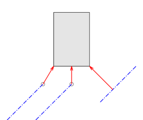
Figure 10: The three possible relative placements of projected paths (line segments) and an outlier pixel (filled rectangle). The distance of the line segment and the rectangle is shown by the corresponding arrows (𝝀𝒂,𝒃,𝒄subscript𝝀𝒂𝒃𝒄{\boldsymbol{\lambda_{a,b,c}}}).

The task is to determine the projected path lengths λisubscript𝜆𝑖\lambda_{i} for each pixel i𝑖i, for a given hit position 𝑷𝑷{\boldsymbol{P}}. Using the coordinates of the two endpoints, find points where the track crosses the horizontal (along x𝑥x direction) or vertical (along y𝑦y direction) pixel division lines. Determine the dominant direction of the cluster by choosing longer projection of the passage to the axes. Sort the endpoints and crossing points along their coordinate in the dominant direction. The lengths of the resulting line segments will give the projected path lengths λisubscript𝜆𝑖\lambda_{i} for touched pixels. In case of outlier pixels determine the distance of the projected line segment to the pixel (Fig. 10) by evaluating the combinations

  • 1.

    two endpoints of the projected path line segment with respect to the four vertices and four edges of the pixel (cases a and b),

  • 2.

    projected path line segment with respect to the four vertices of the pixel (case c),

and choose the negative of the smallest distance. The outlined procedure ensures that by varying the hit position 𝑷𝑷{\boldsymbol{P}}, the projected path lengths of touched and outlier pixels will change continuously, without jumps.
abcRefer to caption𝒏𝟏subscript𝒏1{\boldsymbol{n_{1}}}𝒏𝟐subscript𝒏2{\boldsymbol{n_{2}}}𝝀𝝀{\boldsymbol{\lambda}}
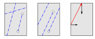
Figure 11: Line segments (dash dotted lines) on the surface of a pixel (filled rectangle). They can be bound by endpoints (open circles) or crossing points. a: The length is insensitive to small change of the hit position. b: The length changes when the hit is moved. c: Normal vectors 𝒏𝟏subscript𝒏1{\boldsymbol{n_{1}}}, 𝒏𝟐subscript𝒏2{\boldsymbol{n_{2}}} and the vector of the projected passage 𝝀𝝀{\boldsymbol{\lambda}}.

3.4 Derivatives

How does the projected path length λ𝜆\lambda change if the hit position 𝑷𝑷{\boldsymbol{P}} is varied? The corresponding line segment can be bound by endpoints or crossing points. The length is insensitive to small changes of the hit position if both points are endpoints or if both points are crossing points on opposite sides of the pixel (Fig. 11 a). The length will change only if one of the points is an endpoint or if both points are crossing points on neighboring sides of the pixel (Fig. 11 b). The derivative λ/𝑷𝜆𝑷\partial\lambda/\partial{\boldsymbol{P}} can be computed with help of the inward directed normal vectors 𝒏𝒋subscript𝒏𝒋{\boldsymbol{n_{j}}} at crossing points and the vector of the projected passage 𝝀𝝀{\boldsymbol{\lambda}} (Fig. 11 c):

λ𝑷=j𝒏𝒋λ|𝒏𝒋𝝀|𝜆𝑷subscript𝑗subscript𝒏𝒋𝜆subscript𝒏𝒋𝝀\frac{\partial\lambda}{\partial{\boldsymbol{P}}}=\sum\limits_{j}\frac{{\boldsymbol{n_{j}}}\lambda}{|{\boldsymbol{n_{j}}}{\boldsymbol{\lambda}}|} (14)

where the index j𝑗j runs for all (0, 1 or 2) crossing points belonging to the line segment. For outliers the derivative is the unit vector

λ𝑷=𝝀λ.𝜆𝑷𝝀𝜆\frac{\partial\lambda}{\partial{\boldsymbol{P}}}=\frac{{\boldsymbol{\lambda}}}{\lambda}. (15)

3.5 Minimization

The joint chi-square for all channels in a hit cluster can be written as

χ2(ε,𝑷)=iχyi2(Δ(ε,li(𝑷)))superscript𝜒2𝜀𝑷subscript𝑖subscriptsuperscript𝜒2subscript𝑦𝑖Δ𝜀subscript𝑙𝑖𝑷\chi^{2}(\varepsilon,{\boldsymbol{P}})=\sum_{i}\chi^{2}_{y_{i}}\left(\Delta(\varepsilon,l_{i}({\boldsymbol{P}}))\right) (16)

where the index i𝑖i runs for all the touched and untouched channels of the hit. Note that while the deposits yisubscript𝑦𝑖y_{i} are given, the ΔΔ\Deltas depend on ε𝜀\varepsilon and the path lengths lisubscript𝑙𝑖l_{i} inside the channels (Eq. (4)) which in turn depend on the actual hit position 𝑷𝑷{\boldsymbol{P}}. The best hit position, and the most probable differential energy loss will be estimated by minimizing χ2superscript𝜒2\chi^{2}. The (three dimensional) path lengths lisubscript𝑙𝑖l_{i} can be obtained from the projected lengths λisubscript𝜆𝑖\lambda_{i} as

li=lλλisubscript𝑙𝑖𝑙𝜆subscript𝜆𝑖l_{i}=\frac{l}{\lambda}\lambda_{i}

where l𝑙l is the total path length and λ𝜆\lambda is the total projected length, both are fixed from the local trajectory direction.
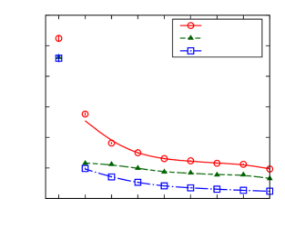
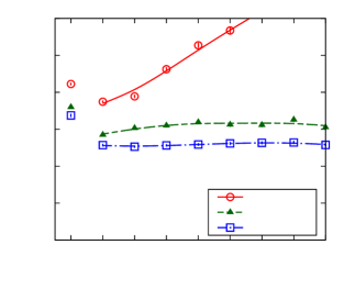
02000400060008000100001200014000-100-80-60-40-20020406080100δsubscript𝛿perpendicular-to\delta_{\perp}[μ𝜇\mum]PixelsRefer to captionWeightedFirst-lastFitter
050010001500200025003000-100-80-60-40-20020406080100δsubscript𝛿parallel-to\delta_{\parallel}[μ𝜇\mum]PixelsRefer to captionWeightedFirst-lastFitter
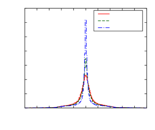
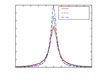
Figure 12: Residuals of the reconstructed hit position in directions perpendicular to (left) or parallel with (right) the projected trajectory using the discussed methods.
0510152025302345678910

σsubscript𝜎perpendicular-to\sigma_{\perp}[μ𝜇\mum]

npixelsubscript𝑛𝑝𝑖𝑥𝑒𝑙n_{pixel}PixelsRefer to captionWeightedFirst-lastFitter
0510152025302345678910

σsubscript𝜎parallel-to\sigma_{\parallel}[μ𝜇\mum]

npixelsubscript𝑛𝑝𝑖𝑥𝑒𝑙n_{pixel}PixelsRefer to captionWeightedFirst-lastFitter
Figure 13: Resolution of the reconstructed hit position in directions perpendicular to (left) or parallel with (right) the projected trajectory using the discussed methods, as a function of the number of pixels in the cluster. Lines are drawn to guide the eye.

In case of hit position estimation the value of ε𝜀\varepsilon is not relevant, hence instead of the complete relationship shown in Eq. (4) a simple linearity can be assumed

Δ(l)εlΔ𝑙𝜀𝑙\Delta(l)\approx\varepsilon l (17)

where ε𝜀\varepsilon is rather the average rate of energy loss. The first derivatives of the χ2superscript𝜒2\chi^{2} components with respect to (ε,𝑷)𝜀𝑷(\varepsilon,{\boldsymbol{P}}) are

χ2εsuperscript𝜒2𝜀\displaystyle\frac{\partial\chi^{2}}{\partial\varepsilon} =χ2Δl,absentsuperscript𝜒2Δ𝑙\displaystyle=\frac{\partial\chi^{2}}{\partial\Delta}l, χ2Pjsuperscript𝜒2subscript𝑃𝑗\displaystyle\frac{\partial\chi^{2}}{\partial P_{j}} =χ2ΔεlPjabsentsuperscript𝜒2Δ𝜀𝑙subscript𝑃𝑗\displaystyle=\frac{\partial\chi^{2}}{\partial\Delta}\varepsilon\frac{\partial l}{\partial P_{j}}

while the second derivatives are

2χ2ε2superscript2superscript𝜒2superscript𝜀2\displaystyle\frac{\partial^{2}\chi^{2}}{\partial\varepsilon^{2}} =2χ2Δ2l2,absentsuperscript2superscript𝜒2superscriptΔ2superscript𝑙2\displaystyle=\frac{\partial^{2}\chi^{2}}{\partial\Delta^{2}}l^{2}, 2χ2PjPksuperscript2superscript𝜒2subscript𝑃𝑗subscript𝑃𝑘\displaystyle\frac{\partial^{2}\chi^{2}}{\partial P_{j}\partial P_{k}} =2χ2Δ2ε2lPjlPkabsentsuperscript2superscript𝜒2superscriptΔ2superscript𝜀2𝑙subscript𝑃𝑗𝑙subscript𝑃𝑘\displaystyle=\frac{\partial^{2}\chi^{2}}{\partial\Delta^{2}}\varepsilon^{2}\frac{\partial l}{\partial P_{j}}\frac{\partial l}{\partial P_{k}}

where the term containing 2l𝑷2=0superscript2𝑙superscript𝑷20\frac{\partial^{2}l}{\partial{\boldsymbol{P}}^{2}}=0 is not shown. The second derivative cross-term is
2χ2εPj=(2χ2Δ2Δ+χ2Δ)lPj.superscript2superscript𝜒2𝜀subscript𝑃𝑗superscript2superscript𝜒2superscriptΔ2Δsuperscript𝜒2Δ𝑙subscript𝑃𝑗\frac{\partial^{2}\chi^{2}}{\partial\varepsilon\partial P_{j}}=\left(\frac{\partial^{2}\chi^{2}}{\partial\Delta^{2}}\Delta+\frac{\partial\chi^{2}}{\partial\Delta}\right)\frac{\partial l}{\partial P_{j}}.\\
05001000150020002500300035004000-100-80-60-40-20020406080100δx𝛿𝑥\delta x[μ𝜇\mum]StripsRefer to captionWeightedFirst-lastFitter
0510152025302345678910

σsubscript𝜎parallel-to\sigma_{\parallel}[μ𝜇\mum]

nstripsubscript𝑛𝑠𝑡𝑟𝑖𝑝n_{strip}StripsRefer to captionWeightedFirst-lastFitter
Figure 14: Residuals of the reconstructed hit position (left) and the resolution of the reconstructed hit position using the discussed methods, as a function of the number of strips in the cluster (right). Lines are drawn to guide the eye.
010002000300040005000600070008000-100-50050100δx𝛿𝑥\delta x[μ𝜇\mum]PixelsRefer to captionFitterPredicted
05001000150020002500-100-50050100δy𝛿𝑦\delta y[μ𝜇\mum]PixelsRefer to captionFitterPredicted
010002000300040005000-100-50050100δx𝛿𝑥\delta x[μ𝜇\mum]StripsRefer to captionFitterPredicted
Figure 15: Residuals of the reconstructed hit position for pixels (x𝑥x and y𝑦y directions) and strips, from left to right. The measured values from comparison of reconstructed and simulated positions (Fitter, dash-dotted line) are shown together with the distribution predicted from the errors of the fitted parameters (Predicted, dashed line).

The partial derivative of the path length is

l𝑷=lλλ𝑷𝑙𝑷𝑙𝜆𝜆𝑷\frac{\partial l}{\partial{\boldsymbol{P}}}=\frac{l}{\lambda}\frac{\partial\lambda}{\partial{\boldsymbol{P}}}

and the last term is given in Eqs. (14) and (15). During minimization the positivity of ε𝜀\varepsilon can be assured by choosing logε𝜀\log\varepsilon as the free parameter. Since both the first and second derivatives can be calculated, Newton’s method [11] can be used for fast and precise minimization.

In case of strips the observed signals are correlated. Before starting with the position estimation the coupling has to be undone first: it will be discussed in Sec. 4.1.

Table 2: Some relevant quantities used in silicon detector simulation.
Detector thickness 300 μ𝜇\mum
Pitch, pixels (x𝑥x direction) 100 μ𝜇\mum
Pitch, pixels (y𝑦y direction) 200 μ𝜇\mum
Pitch, strips 100 μ𝜇\mum
Signal coupling, strips 0.1
Channel noise 1.5 keV
Channel threshold 7.5 keV
Channel saturation 150 keV

3.6 Results

For the studies in Sec. 3 and 4 charged particles in the βγ𝛽𝛾\beta\gamma range of 0.56 – 10.0 were generated with flat distribution in log(βγ)𝛽𝛾\log(\beta\gamma), and in pseudo-rapidity, 2.5<η<2.52.5𝜂2.5-2.5<\eta<2.5, following a pTexp(pT/T)subscript𝑝𝑇subscript𝑝𝑇𝑇p_{T}\exp(-p_{T}/T) shape for the transverse momentum distribution, where T=0.15GeV/c𝑇0.15GeV𝑐T=0.15~{}\mathrm{GeV}/c was set. Some relevant quantities used in the simulation are given in Table 2. The pixel and strip layers were located in a barrel geometry at 10 cm and 50 cm radial distances from the beam axis, respectively, in a B=𝐵absentB= 4 T magnetic field. 100 000 complete pixel and strip hits were generated, down to the level of individual channels. For simplicity, the charge drift direction was assumed to be parallel with the electric field, perpendicular to the silicon unit. Hence the change in direction due to the 𝑬×𝑩𝑬𝑩{\boldsymbol{E}}\times{\boldsymbol{B}} effect was omitted.

The addition of local particle direction and energy loss information will make the residuals of the hit position measurement smaller. In case of pixels the deviations from the true value can be decomposed into projections parallel and perpendicular to the passage of the particle (Fig. 12). In both cases the proposed model (labeled as Fitter) gives better results than the weighted or first-last methods introduced in Sec. 3.1. The differences are mostly seen in the perpendicular direction. The measured Gaussian resolutions as a function of the number of pixels in the cluster for all three discussed methods are shown in Fig. 13, in some cases reaching 1 μ𝜇\mum levels. The corresponding plots of residuals and position resolution for strips are shown in Fig. 14, again the fitter giving the best results.
024681012020406080100120

ydelimited-⟨⟩𝑦\langle y\rangle[keV]

l [μ𝜇\mum]βγ=3.16𝛽𝛾3.16\beta\gamma=3.16Refer to captiont=𝑡absentt=6 keVt=𝑡absentt=8 keVt=𝑡absentt=10 keV
0100200300400500050100150200

ydelimited-⟨⟩𝑦\langle y\rangle[keV]

l [μ𝜇\mum]βγ=0.32𝛽𝛾0.32\beta\gamma=0.32Refer to captiont=𝑡absentt=100 keVt=𝑡absentt=150 keVt=𝑡absentt=200 keV
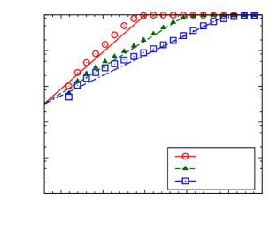
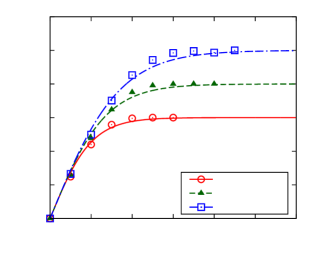
Figure 16: The average lost deposit ydelimited-⟨⟩𝑦\langle y\rangle as function of the path length l𝑙l for several threshold. Left: deposits below threshold with t=𝑡absentt= 6, 8 and 10 keV, for particles with βγ=3.16𝛽𝛾3.16\beta\gamma=3.16. Right: deposits above censoring level with t=𝑡absentt= 100, 150 and 200 keV, for particles with βγ=0.32𝛽𝛾0.32\beta\gamma=0.32. The curves show the functional forms of Eq. (18) and Eq. (19), respectively.

The resolution of the position estimate can be calculated hit by hit using the observed Fisher information (Sec. 2.4). Residuals of the reconstructed hit position for pixels and strips are shown in Fig. 15. The measured values from comparison of reconstructed and simulated positions are plotted together with the distribution predicted from the errors of the fitted parameters. There is a very good agreement between observed and predicted values. Note that for pixels the cross-correlation term can also be deduced giving valuable input for track refit.

4 Estimation of hit energy deposit

The deposited energy Q𝑄Q in the cluster could be plainly estimated with the sum of the individual channel deposits yisubscript𝑦𝑖y_{i}:

QSum=iyisubscript𝑄Sumsubscript𝑖subscript𝑦𝑖Q_{\mathrm{Sum}}=\sum_{i}y_{i}

but this approach clearly has various biases (Sec. 2.2).

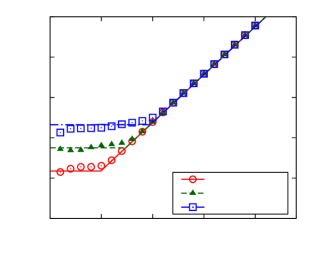
The deposited energy can be lost during clustering, because the deposit can be below the channel threshold (left truncation). The average lost deposit ydelimited-⟨⟩𝑦\langle y\rangle can be estimated using the discussed microscopical model. Example values as function of path length l𝑙l for several threshold settings (t=𝑡absentt= 6, 8 and 10 keV) are shown in Fig. 16-left, for particles with βγ=3.16𝛽𝛾3.16\beta\gamma=3.16. In case of large l𝑙l the average lost deposit is close to the threshold, ytdelimited-⟨⟩𝑦𝑡\langle y\rangle\approx t, because the probability density function p(y|l)𝑝conditional𝑦𝑙p(y|l) is very steep for low y𝑦y values. If the path length l𝑙l is small the average lost deposit will be simply yεldelimited-⟨⟩𝑦𝜀𝑙\langle y\rangle\approx\varepsilon l. These observations can be successfully described and matched with simulated data (Fig. 16-left) using the following formula:

yy<tttanh(εlt).subscriptdelimited-⟨⟩𝑦𝑦𝑡𝑡𝜀𝑙𝑡\langle y\rangle_{y<t}\approx t\tanh\left(\frac{\varepsilon l}{t}\right). (18)
0200400600800100012001400-20-15-10-505101520δΔ𝛿Δ\delta\Delta[keV]PixelsRefer to captionSumFitter
05001000150020002500300035004000-20-15-10-505101520δΔ𝛿Δ\delta\Delta[keV]StripsRefer to captionSumFitter
Figure 17: Residuals of the reconstructed deposited energy of the hit cluster for pixels (left) and strips (right). The result of the simple sum and the proposed fitter are compared.

The measured value can also be saturated, when the deposit is above censoring level (right censoring). Example values as function of path length l𝑙l for several threshold settings (t=𝑡absentt= 100, 150 and 200 keV) are shown in Fig. 16-right, for particles with βγ=0.32𝛽𝛾0.32\beta\gamma=0.32. In case of small l𝑙l the average lost deposit can be estimated as

ytyexp[νy/σΔ(t)]texp[νy/σΔ(t)]=t+σΔ(t)ν.delimited-⟨⟩𝑦subscript𝑡𝑦𝜈𝑦subscript𝜎Δ𝑡subscript𝑡𝜈𝑦subscript𝜎Δ𝑡𝑡subscript𝜎Δ𝑡𝜈\langle y\rangle\approx\frac{\int_{t}y\exp\left[-\nu y/\sigma_{\Delta}(t)\right]}{\int_{t}\phantom{y}\exp\left[-\nu y/\sigma_{\Delta}(t)\right]}=t+\frac{\sigma_{\Delta}(t)}{\nu}.

If the path length l𝑙l is large the average lost deposit will be simply yεldelimited-⟨⟩𝑦𝜀𝑙\langle y\rangle\approx\varepsilon l. These observations can be successfully described and matched with simulated data (Fig. 16-right) using the following formula:

yy>tmax(t+σΔ(t)ν,εl).subscriptdelimited-⟨⟩𝑦𝑦𝑡𝑡subscript𝜎Δ𝑡𝜈𝜀𝑙\langle y\rangle_{y>t}\approx\max\left(t+\frac{\sigma_{\Delta}(t)}{\nu},\varepsilon l\right). (19)

4.1 Coupled signals

In case of strips the observed signals are correlated due to the capacitive coupling of the neighboring strips and cross-talk. This effect can be modelled by a tridiagonal matrix:

C=(12αα0α12αα0α12α)𝐶matrix12𝛼𝛼missing-subexpression0𝛼12𝛼missing-subexpressionmissing-subexpression𝛼0missing-subexpression𝛼12𝛼\displaystyle C=\begin{pmatrix}1-2\alpha&\alpha&&0\\ \alpha&1-2\alpha&\ddots&\\ &\ddots&\ddots&\alpha\\ 0&&\alpha&1-2\alpha\end{pmatrix}
where α>0𝛼0\alpha>0, such that the measured deposits ysuperscript𝑦y^{\prime} can be obtained from the original ones y𝑦y by
𝒚=C𝒚.superscript𝒚bold-′𝐶𝒚\displaystyle{\boldsymbol{y^{\prime}}}=C{\boldsymbol{y}}.

Since the signals are coupled, iχi2subscript𝑖superscriptsubscript𝜒𝑖2\sum_{i}\chi_{i}^{2} would sum dependent values making the minimization false. The coupling should be first undone by applying C1superscript𝐶1C^{-1} to the measured deposits. The inverse of C𝐶C can be exactly calculated [12], furthermore if α1much-less-than𝛼1\alpha\ll 1 it is well approximated by

C1ij=(21/α)|ij|1α.subscriptsuperscript𝐶1𝑖𝑗superscript21𝛼𝑖𝑗1𝛼{C^{-1}}_{ij}=-\frac{(2-1/\alpha)^{|i-j|-1}}{\alpha}.

Note that due to the presence of signals below threshold and saturated values the decoupling is not exact. The measured deposit in the i𝑖ith channel is either given, or subject to inequalities:

(C𝒚)i=yisubscript𝐶𝒚𝑖superscriptsubscript𝑦𝑖\displaystyle(C{\boldsymbol{y}})_{i}=y_{i}^{\prime} or (C𝒚)i<tsubscript𝐶𝒚𝑖𝑡\displaystyle(C{\boldsymbol{y}})_{i}<t or (C𝒚)i>t.subscript𝐶𝒚𝑖𝑡\displaystyle(C{\boldsymbol{y}})_{i}>t.

In that sense a system of equalities and inequalities has to be solved for 𝒚𝒚{\boldsymbol{y}}. The problem can be easily handled with the tools of linear programming [11, 13], the OOQP package [14], available in ROOT [15] under MATH/QUADP, could be used for this purpose. The solution is not unique, hence the minimization of a scalar product 𝒄𝒚𝒄superscript𝒚bold-′{\boldsymbol{c}}{\boldsymbol{y^{\prime}}} is also required. In this case it is advantageous to set 𝒄=𝒄absent{\boldsymbol{c}}= (1, …, 1). This way those solution will be selected where iyiQFittersubscript𝑖subscript𝑦𝑖subscript𝑄Fitter\sum_{i}y_{i}\equiv Q_{\mathrm{Fitter}} is minimal.

In fact the situation is even more complicated due to the presence of detector and readout noise. Assuming a Gaussian noise with standard deviation σ𝜎\sigma, the χ2superscript𝜒2\chi^{2} contribution of the i𝑖ith channel is

χy2subscriptsuperscript𝜒2superscript𝑦\displaystyle\chi^{2}_{y^{\prime}} =(yi(Cy)iσ)2absentsuperscriptsuperscriptsubscript𝑦𝑖subscript𝐶𝑦𝑖𝜎2\displaystyle=\left(\frac{y_{i}^{\prime}-(Cy)_{i}}{\sigma}\right)^{2}
χy<t2subscriptsuperscript𝜒2superscript𝑦𝑡\displaystyle\chi^{2}_{y^{\prime}<t} {12(t(Cy)iσ2)2,if t(Cy)iσ2<00,otherwiseabsentcases12superscript𝑡subscript𝐶𝑦𝑖𝜎22if t(Cy)iσ2<00otherwise\displaystyle\approx\begin{cases}\frac{1}{2}\left(\frac{t-(Cy)_{i}}{\sigma}-2\right)^{2},&\text{if $\frac{t-(Cy)_{i}}{\sigma}-2<0$}\\ 0,&\text{otherwise}\end{cases}
χy>t2subscriptsuperscript𝜒2superscript𝑦𝑡\displaystyle\chi^{2}_{y^{\prime}>t} {12(t(Cy)iσ+2)2,if t(Cy)iσ+2>00,otherwise.absentcases12superscript𝑡subscript𝐶𝑦𝑖𝜎22if t(Cy)iσ+2>00otherwise\displaystyle\approx\begin{cases}\frac{1}{2}\left(\frac{t-(Cy)_{i}}{\sigma}+2\right)^{2},&\text{if $\frac{t-(Cy)_{i}}{\sigma}+2>0$}\\ 0,&\text{otherwise}.\end{cases}

Here, in case of the inequalities, the exact values

P(y<t|m)=12[1+erf(tmσ2)]𝑃𝑦bra𝑡𝑚12delimited-[]1erf𝑡𝑚𝜎2\displaystyle P(y<t|m)=\frac{1}{2}\left[1+\operatorname{erf}\left(\frac{t-m}{\sigma\sqrt{2}}\right)\right]
were approximated as
χ2=2logP{12(tmσ2)2,if tmσ2<00,otherwise.superscript𝜒22𝑃cases12superscript𝑡𝑚𝜎22if tmσ2<00otherwise\displaystyle\chi^{2}=-2\log P\approx\begin{cases}\frac{1}{2}\left(\frac{t-m}{\sigma}-2\right)^{2},&\text{if $\frac{t-m}{\sigma}-2<0$}\\ 0,&\text{otherwise}.\end{cases}

In order to keep the minimization away from unphysical negative yisubscript𝑦𝑖y_{i} values, a penalty (C𝒚)i/σ)2(C{\boldsymbol{y}})_{i}/\sigma)^{2} is added if (C𝒚)i<0subscript𝐶𝒚𝑖0(C{\boldsymbol{y}})_{i}<0.

The joint chi-square χyi2subscriptsuperscript𝜒2superscriptsubscript𝑦𝑖\sum\chi^{2}_{y_{i}^{\prime}} is a positive definite quadratic function of the original deposits yisubscript𝑦𝑖y_{i}. The first and second derivatives with respect to yisubscript𝑦𝑖y_{i} components are easily calculable and the function can be minimized with Newton’s method, in few iterative steps.

If some yisubscript𝑦𝑖y_{i} values are negative at the minimum, the one with lowest value is fixed to 0, the minimization is redone. In the end we have a minimum joint chi-square with all the yisubscript𝑦𝑖y_{i} values being non-negative. At the minimum the total charge and its variance are given as

Q𝑄\displaystyle Q =iyi,absentsubscript𝑖subscript𝑦𝑖\displaystyle=\sum_{i}y_{i}, σQ2superscriptsubscript𝜎𝑄2\displaystyle\sigma_{Q}^{2} =i,jVar(yi,yj),absentsubscript𝑖𝑗Varsubscript𝑦𝑖subscript𝑦𝑗\displaystyle=\sum_{i,j}\mathrm{Var}(y_{i},y_{j}),

respectively.

4.2 Results

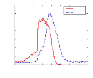
The details of the simulation are the same as they were described in Sec. 3.6. Residuals of the reconstructed deposited energy of the hit cluster are shown in Fig. 17, for pixels and strips. The result of the simple sum and the proposed fitter are compared. The sum has a 55-5 keV shift for both configurations which is a 5% effect for minimum ionizing particles along a 300 μ𝜇\mum path in silicon. At the same time the fitter has practically no bias and a better resolution.

5 Estimation of the most probable differential energy loss for tracks

Having the proper hit energy deposits yisubscript𝑦𝑖y_{i}, the next step is to estimate the most probable differential energy loss for the whole trajectory. The task is very similar (Eq. (16)), but only ε𝜀\varepsilon has to be optimized, because the path lengths lisubscript𝑙𝑖l_{i} are given from track finding,

χ2(ε)=iχyi2(Δ(ε,li)).superscript𝜒2𝜀subscript𝑖subscriptsuperscript𝜒2subscript𝑦𝑖Δ𝜀subscript𝑙𝑖\chi^{2}(\varepsilon)=\sum_{i}\chi^{2}_{y_{i}}\left(\Delta(\varepsilon,l_{i})\right).

Since the terms on the right contain linear or positive definite quadratic functions (Eqs. (11)-(13)) a fast convergence with Newton’s method is guaranteed.

The derivatives are

χy2(Δ)Δsubscriptsuperscript𝜒2𝑦ΔΔ\displaystyle\frac{\partial\chi^{2}_{y}(\Delta)}{\partial\Delta} ={2νσΔ(y),if Δ<yνσΔ(y)2(Δy)σΔ(y)2,if ΔyνσΔ(y)absentcases2𝜈subscript𝜎Δ𝑦if Δ<yνσΔ(y)2Δ𝑦subscript𝜎Δsuperscript𝑦2if ΔyνσΔ(y)\displaystyle=\begin{cases}\frac{-2\nu}{\sigma_{\Delta}(y)},&\hskip 18.06749pt\text{if $\Delta<y-\nu\sigma_{\Delta}(y)$}\\ \frac{2(\Delta-y)}{\sigma_{\Delta}(y)^{2}},&\hskip 18.06749pt\text{if $\Delta\geq y-\nu\sigma_{\Delta}(y)$}\end{cases}
χy<t2(Δ)Δsubscriptsuperscript𝜒2𝑦𝑡ΔΔ\displaystyle\frac{\partial\chi^{2}_{y<t}(\Delta)}{\partial\Delta} ={0,if Δ<tσΔ(t)2(Δt+σΔ(t))σΔ(t)2,if ΔtσΔ(t)absentcases0if Δ<tσΔ(t)2Δ𝑡subscript𝜎Δ𝑡subscript𝜎Δsuperscript𝑡2if ΔtσΔ(t)\displaystyle=\begin{cases}0,&\text{if $\Delta<t-\sigma_{\Delta}(t)$}\\ \frac{2(\Delta-t+\sigma_{\Delta}(t))}{\sigma_{\Delta}(t)^{2}},&\text{if $\Delta\geq t-\sigma_{\Delta}(t)$}\end{cases}
χy>t2(Δ)Δsubscriptsuperscript𝜒2𝑦𝑡ΔΔ\displaystyle\frac{\chi^{2}_{y>t}(\Delta)}{\partial\Delta} ={1σΔ(t),if Δ<t+σΔ(t)0,if Δt+σΔ(t).absentcases1subscript𝜎Δ𝑡if Δ<t+σΔ(t)0if Δt+σΔ(t)\displaystyle=\begin{cases}-\frac{1}{\sigma_{\Delta}(t)},&\hskip 18.06749pt\text{if $\Delta<t+\sigma_{\Delta}(t)$}\\ 0,&\hskip 18.06749pt\text{if $\Delta\geq t+\sigma_{\Delta}(t)$}.\end{cases}

Only the following second derivatives are non-zero:

2χy2(Δ)Δ2superscript2subscriptsuperscript𝜒2𝑦ΔsuperscriptΔ2\displaystyle\frac{\partial^{2}\chi^{2}_{y}(\Delta)}{\partial\Delta^{2}} =2σΔ(y)2,absent2subscript𝜎Δsuperscript𝑦2\displaystyle=\frac{2}{\sigma_{\Delta}(y)^{2}}, if ΔyνσΔ(y)Δ𝑦𝜈subscript𝜎Δ𝑦\Delta\geq y-\nu\sigma_{\Delta}(y)
2χy<t2(Δ)Δ2superscript2subscriptsuperscript𝜒2𝑦𝑡ΔsuperscriptΔ2\displaystyle\frac{\partial^{2}\chi^{2}_{y<t}(\Delta)}{\partial\Delta^{2}} =2σΔ(t)2,absent2subscript𝜎Δsuperscript𝑡2\displaystyle=\frac{2}{\sigma_{\Delta}(t)^{2}}, if ΔtσΔ(t).if ΔtσΔ(t)\displaystyle\text{if $\Delta\geq t-\sigma_{\Delta}(t)$}.
104superscript10410^{-4}103superscript10310^{-3}102superscript10210^{-2}101superscript10110^{-1}1002003004005006007008009001000

σΔ2delimited-⟨⟩superscriptsubscript𝜎Δ2\left\langle\sigma_{\Delta}^{-2}\right\rangle[keV2superscriptkeV2\mathrm{keV^{-2}}]

l𝑙l[μ𝜇\mum]nε=1.58±0.02subscript𝑛𝜀plus-or-minus1.580.02n_{\varepsilon}=-1.58\pm 0.02nl=1.75±0.02subscript𝑛𝑙plus-or-minus1.750.02n_{l}=-1.75\pm 0.02Refer to captionβγ=0.56𝛽𝛾0.56\beta\gamma=0.56βγ=1.00𝛽𝛾1.00\beta\gamma=1.00βγ=3.16𝛽𝛾3.16\beta\gamma=3.16βγ=10.0𝛽𝛾10.0\beta\gamma=10.0
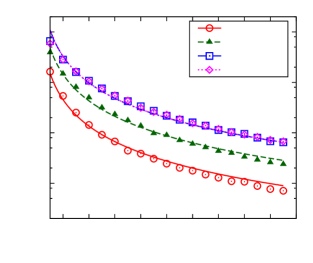
Figure 18: The expectation value of σΔ2superscriptsubscript𝜎Δ2\sigma_{\Delta}^{-2} as function of path length l𝑙l at several βγ𝛽𝛾\beta\gamma values (points). The curves show the functional form defined in Eq. (20). The corresponding fitted powers for ε𝜀\varepsilon and l𝑙l are also indicated.

5.1 Resolution

The dependence of the standard deviation of the ε𝜀\varepsilon estimate can be obtained as (Sec. 2.4):

(ε)=12iE[2χi2ε2]𝜀12subscript𝑖𝐸delimited-[]superscript2superscriptsubscript𝜒𝑖2superscript𝜀2\displaystyle{\cal I}(\varepsilon)=\frac{1}{2}\sum_{i}E\left[\frac{\partial^{2}\chi_{i}^{2}}{\partial\varepsilon^{2}}\right]
where the second derivative is
122χi2ε2={(li[1+alog(li/l0)]σΔ(y))2,if in the Gaussian part0,if in the exponential part.12superscript2superscriptsubscript𝜒𝑖2superscript𝜀2casessuperscriptsubscript𝑙𝑖delimited-[]1𝑎subscript𝑙𝑖subscript𝑙0subscript𝜎Δ𝑦2if in the Gaussian part0if in the exponential part.\displaystyle\frac{1}{2}\frac{\partial^{2}\chi_{i}^{2}}{\partial\varepsilon^{2}}=\begin{cases}\left(\frac{l_{i}[1+a\log(l_{i}/l_{0})]}{\sigma_{\Delta}(y)}\right)^{2},&\text{if in the Gaussian part}\\ 0,&\text{if in the exponential part.}\\ \end{cases}

According to the fit shown in Fig. 18 the expectation value of σΔ2superscriptsubscript𝜎Δ2\sigma_{\Delta}^{-2} is a power function of ε𝜀\varepsilon and l𝑙l:

σΔ2ε1.6l1.8.proportional-todelimited-⟨⟩superscriptsubscript𝜎Δ2superscript𝜀1.6superscript𝑙1.8\left\langle\sigma_{\Delta}^{-2}\right\rangle\propto\varepsilon^{-1.6}l^{-1.8}. (20)
01000200030004000500060000.811.21.41.61.8

Reconstructed relative gain

log\log(ε𝜀\varepsilon [MeV/cm])300 μ𝜇\mumRefer to captionFitterTruncatedPower (-2)Harmonic (-1)Arithmetic (1)
01000200030004000500060000.811.21.41.61.8

Reconstructed relative gain

log\log(ε𝜀\varepsilon [MeV/cm])300-600 μ𝜇\mumRefer to captionFitterTruncatedPower (-2)Harmonic (-1)Arithmetic (1)
010002000300040005000600070000.811.21.41.61.8

Reconstructed relative gain

log\log(ε𝜀\varepsilon [MeV/cm])300-900 μ𝜇\mumRefer to captionFitterTruncatedPower (-2)Harmonic (-1)Arithmetic (1)
010002000300040005000600070000.811.21.41.61.8

Reconstructed relative gain

log\log(ε𝜀\varepsilon [MeV/cm])300-1200 μ𝜇\mumRefer to captionFitterTruncatedPower (-2)Harmonic (-1)Arithmetic (1)
Figure 19: Distribution of the estimated most probable differential energy loss values at reference length (ε𝜀\varepsilon), obtained with the four detector layer settings. Several methods are shown: this maximum likelihood fitter, truncated mean, power mean (power -2), harmonic mean (-1) and arithmetic mean (1).

With that, also approximating the factor alog(li/l0)𝑎subscript𝑙𝑖subscript𝑙0a\log(l_{i}/l_{0}) in the range l=𝑙absentl= 50 – 1000 μ𝜇\mum,

σ2(ε)ε1.6ili0.2.proportional-tosuperscript𝜎2𝜀superscript𝜀1.6subscript𝑖superscriptsubscript𝑙𝑖0.2\sigma^{2}(\varepsilon)\propto\frac{\varepsilon^{1.6}}{\sum_{i}l_{i}^{0.2}}.

It is clear that the relative resolution σ(ε)/ε𝜎𝜀𝜀\sigma(\varepsilon)/\varepsilon only slightly depends on ε𝜀\varepsilon, hence logε𝜀\log\varepsilon is a convenient and uniform estimator. Since the exponent of the path length is also small (0.2), it is not the total thickness of the silicon, but the number of independent measurements that matters. For a given total path length the relative resolution is proportional to n0.4superscript𝑛0.4n^{-0.4}, where n𝑛n is the number of independent measurements. The reason for that originates in the non-Gaussian nature of the energy deposit distribution. Grouped measurements would have worse resolution unlike in the Gaussian case where the resolution would stay unchanged.

5.2 False hit removal

Since the association of hits to trajectories is not always unambiguous some hits do not belong to the proper track. Although their measured deposit is correct, the calculated path length can be false. Assuming that there is at most one false hit in a trajectory it can be detected and removed: the exclusion of the outlier hit decreases the joint chi-square of the trajectory by a considerable amount.
345678

300 μ𝜇\mum

300–600 μ𝜇\mum

300–900 μ𝜇\mum

300–1200 μ𝜇\mum

Pion-kaon separation

Refer to captionFitterTruncatedPower (-2)Harmonic (-1)
0.911.11.21.3

300 μ𝜇\mum

300–600 μ𝜇\mum

300–900 μ𝜇\mum

300–1200 μ𝜇\mum

log\log(ε𝜀\varepsilon [MeV/cm])

Refer to captionFitterTruncatedPower (-2)Harmonic (-1)
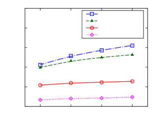
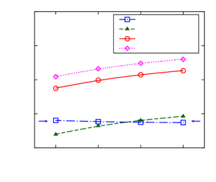
Figure 20: Left: pion-kaon separation power for four detector layer settings, using several methods: this maximum likelihood fitter, truncated mean, power mean (power -2), and harmonic mean (-1). Right: most probable differential energy loss values at reference length (logε𝜀\log\varepsilon), shown for the four detector layer settings. The horizontal arrows show the expected theoretical value. Lines are drawn to guide the eye.

5.3 Distribution of the estimator

Although the most probable value of ε𝜀\varepsilon is estimated, it is equally important to deduce, or also estimate, its distribution. Although the variance of the estimate is given, the original probability density is a skewed function: the estimator is not expected to follow a perfect Gaussian distribution. The distribution of the joint χ2superscript𝜒2\chi^{2} could be determined track by track with detailed Monte Carlo simulation, but this possibility would have huge computational demands and timing issues.

Are there other methods that could be used to estimate the distribution of the estimator? One of them is the statistical bootstrap [16], that is a random sampling with replacement from the original dataset. The so called jackknife method [16] can also be considered where the estimate is systematically recomputed leaving out one observation at a time from the sample. Both methods can be used to estimate bias, variance and the shape of the distributions. It can be shown that the jackknife method cancels biases with terms proportional to 1/n1𝑛1/n and 1/n21superscript𝑛21/n^{2}. A problem common to both resampling methods is that they do not work if the sample size is small. Since here we deal sometimes with tracks with as few as two or three measurements these approaches are not viable. For example, in case of the jackknife method, the variance of the subsamples will have large errors if the subsample consist of only one or two measurements.

As a solution, the shape of the logε𝜀\log\varepsilon distribution could be determined by energy deposit regeneration. A measured track is used to construct the shape distribution of a given particle species (mass m𝑚m), if its measured ε𝜀\varepsilon value is compatible with the corresponding value at a given p/m𝑝𝑚p/m. While all kinematical parameters and path lengths of hits in silicon are kept, all energy deposit values are randomly regenerated using assumed p/m𝑝𝑚p/m values, as described in Sec. 2.5. The chosen procedure ensures meaningful shape determination even for tracks with very few hits and exploits the success of the energy loss model seen at the hit level.

5.4 Results

In order to demonstrate track level applications a very simple detector model was used: 16 layers of silicon at normal incidence. The orientation of layers and the bending of particle trajectories are taken into account by defining four different layer settings:

  • 1.

    all layers are 300 μ𝜇\mum thick (labeled as 300 μ𝜇\mum);

  • 2.

    four groups of layers, each containing four 300, 400, 500 and 600 μ𝜇\mum thick layers (300-600 μ𝜇\mum);

  • 3.

    four groups of layers, each containing four 300, 500, 700 and 900 μ𝜇\mum thick layers (300-900 μ𝜇\mum);

  • 4.

    four groups of layers, each containing four 300, 600, 900 and 1200 μ𝜇\mum thick layers (300-1200 μ𝜇\mum).

For the study the 100 000 pions and 30 000 kaons were generated at total momentum p=0.8GeV/c𝑝0.8GeV𝑐p=0.8~{}\mathrm{GeV}/c, and a Gaussian noise with 1 keV standard deviation was added to each energy deposit.

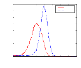
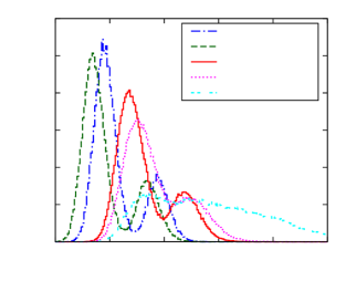
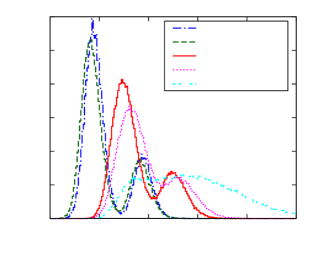
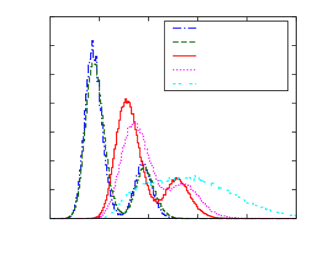
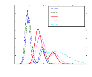
Distribution of the estimated most probable differential energy loss values at reference length (logε𝜀\log\varepsilon), obtained with the four detector layer settings, are shown in Fig. 19 (Fitter). Results of several other methods working with the differential energy deposit values yi/lisubscript𝑦𝑖subscript𝑙𝑖y_{i}/l_{i} are also plotted: truncated mean (average of the lowest half of the yi/lisubscript𝑦𝑖subscript𝑙𝑖y_{i}/l_{i} numbers, 0-50% truncation) [17, 18]; as well as those using all measurements, such as power mean (power -2), harmonic mean (power -1) and arithmetic mean (power 1). While the maximum likelihood fitter gives the best results in all the cases, power means have much worse resolution. The truncated mean performs surprisingly well.

The resulted distributions can be fitted with sum of Gaussians. The performance can be further examined by plotting the pion-kaon separation power, defined as |m1m2|/[(σ12+σ22)/2]1/2subscript𝑚1subscript𝑚2superscriptdelimited-[]superscriptsubscript𝜎12superscriptsubscript𝜎22212|m_{1}-m_{2}|/[(\sigma_{1}^{2}+\sigma_{2}^{2})/2]^{1/2}, where misubscript𝑚𝑖m_{i} and σisubscript𝜎𝑖\sigma_{i} are the means and standard deviations for pions and kaons, respectively. Comparisons including estimators listed above are shown in Fig. 20-left, for the four detector layers settings. Again the maximum likelihood fitter gives the best result over the others. The separation power increases if longer hit path lengths or thicker detectors are used (compare with observations in Sec. 5.1).

Ideally the mean of the logε𝜀\log\varepsilon estimates should not depend on path lengths and detector details. The dependence of the mean for the four layers settings is given in Fig. 20-right. The horizontal arrows show the expected theoretical value. It is clear that the maximum likelihood fitter provides stable means, while the others show a pronounced increase. Although for these latter the dependencies could be compensated, in case of tracks with varying path length distribution only the proposed method would perform appropriately.

6 Detector gain calibration with tracks

In order to determine the multiplicative gain correction g𝑔g for a chip, terms such as

Xj2(g)χgyj2(Δ)superscriptsubscript𝑋𝑗2𝑔subscriptsuperscript𝜒2𝑔subscript𝑦𝑗ΔX_{j}^{2}(g)\equiv\chi^{2}_{gy_{j}}(\Delta)

should be summed for collected hits and the sum minimized by varying g𝑔g. The partial derivatives of χy2subscriptsuperscript𝜒2𝑦\chi^{2}_{y} are

χy2(Δ)ysubscriptsuperscript𝜒2𝑦Δ𝑦\displaystyle\frac{\partial\chi^{2}_{y}(\Delta)}{\partial y} =2bσΔ(y)+{2νσΔ(Δ)σΔ(y)2,if Δ<yνσΔ(y)2(Δy)σΔ(Δ)σΔ(y)3,if ΔyνσΔ(y)absent2𝑏subscript𝜎Δ𝑦cases2𝜈subscript𝜎ΔΔsubscript𝜎Δsuperscript𝑦2if Δ<yνσΔ(y)2Δ𝑦subscript𝜎ΔΔsubscript𝜎Δsuperscript𝑦3if ΔyνσΔ(y)\displaystyle=\;\;\frac{2b}{\sigma_{\Delta}(y)}+\begin{cases}\frac{2\nu\sigma_{\Delta}(\Delta)}{\sigma_{\Delta}(y)^{2}},&\text{if $\Delta<y-\nu\sigma_{\Delta}(y)$}\\ -\frac{2(\Delta-y)\sigma_{\Delta}(\Delta)}{\sigma_{\Delta}(y)^{3}},&\text{if $\Delta\geq y-\nu\sigma_{\Delta}(y)$}\end{cases}
2χy2(Δ)y2superscript2subscriptsuperscript𝜒2𝑦Δsuperscript𝑦2\displaystyle\frac{\partial^{2}\chi^{2}_{y}(\Delta)}{\partial y^{2}} =2b2σΔ(y)2+absentlimit-from2superscript𝑏2subscript𝜎Δsuperscript𝑦2\displaystyle=-\frac{2b^{2}}{\sigma_{\Delta}(y)^{2}}+
+\displaystyle+ {4νbσΔ(Δ)σΔ(y)3,if Δ<yνσΔ(y)2[σΔ(y)+3b(Δy)]σΔ(Δ)σΔ(y)4,if ΔyνσΔ(y).cases4𝜈𝑏subscript𝜎ΔΔsubscript𝜎Δsuperscript𝑦3if Δ<yνσΔ(y)2delimited-[]subscript𝜎Δ𝑦3𝑏Δ𝑦subscript𝜎ΔΔsubscript𝜎Δsuperscript𝑦4if ΔyνσΔ(y)\displaystyle\begin{cases}-\frac{4\nu b\sigma_{\Delta}(\Delta)}{\sigma_{\Delta}(y)^{3}},&\text{if $\Delta<y-\nu\sigma_{\Delta}(y)$}\\ \frac{2\left[\sigma_{\Delta}(y)+3b(\Delta-y)\right]\sigma_{\Delta}(\Delta)}{\sigma_{\Delta}(y)^{4}},&\text{if $\Delta\geq y-\nu\sigma_{\Delta}(y)$}.\end{cases}

With that

Xj2gsuperscriptsubscript𝑋𝑗2𝑔\displaystyle\frac{\partial X_{j}^{2}}{\partial g} =(ygχ2y)|y=gyjabsentevaluated-at𝑦𝑔superscript𝜒2𝑦𝑦𝑔subscript𝑦𝑗\displaystyle=\left(\frac{y}{g}\frac{\partial\chi^{2}}{\partial y}\right)\Bigg{|}_{y=gy_{j}}
2Xj2g2superscript2superscriptsubscript𝑋𝑗2superscript𝑔2\displaystyle\frac{\partial^{2}X_{j}^{2}}{\partial g^{2}} =(y2g22χ2y2)|y=gyjabsentevaluated-atsuperscript𝑦2superscript𝑔2superscript2superscript𝜒2superscript𝑦2𝑦𝑔subscript𝑦𝑗\displaystyle=\left(\frac{y^{2}}{g^{2}}\frac{\partial^{2}\chi^{2}}{\partial y^{2}}\right)\Bigg{|}_{y=gy_{j}}

where y=gyj𝑦𝑔subscript𝑦𝑗y=gy_{j} should be substituted.

6.1 Complete gain calibration

The cross-calibration can be performed in the following steps.

  1. 1.

    With help of a preliminary gain calibration estimate ε𝜀\varepsilon for each track. Select pion-like tracks and collect the values of βγ𝛽𝛾\beta\gamma, path length and deposit of each hit, and store them for every chip separately. For each chip minimize the joint chi-square of all selected hits by varying the gains. The minimization is best performed by a golden section search [19] first, in order to get near the region of the minimum, followed by a refinement using Newton’s method.

  2. 2.

    Using the updated gains select only those tracks which are certainly pions, kaons, protons or decay daughters of abundantly produced hadrons (KS0π+πsubscriptsuperscriptK0Ssuperscript𝜋superscript𝜋\mathrm{K^{0}_{S}}\rightarrow\mathrm{\pi^{+}}\mathrm{\pi^{-}}, ΛpπΛpsuperscript𝜋\mathrm{\Lambda}\rightarrow\mathrm{p}\mathrm{\pi^{-}}, Λ¯p¯π+¯Λ¯psuperscript𝜋\mathrm{\overline{\Lambda}}\rightarrow\mathrm{\overline{p}}\mathrm{\pi^{+}}), or conversion products (γe+e𝛾superscriptesuperscripte\mathrm{\gamma}\rightarrow\mathrm{e}^{+}\mathrm{e}^{-}). Collect their hits for every chip separately and minimize again the joint chi-square chip by chip by varying the gains with similar methods as above.

  3. 3.

    Finally, using all tracks, minimize the their joint chi-square simultaneously. This can be accomplished by nested minimizations. For a given set of gains the εisubscript𝜀𝑖\varepsilon_{i} values are determined for each track separately in the course of a local minimization. The gains of chips can be highly correlated since tracks often traverse detector units which are behind each other or very close in space (double-sided units), but also due to manufacturing details. In case of 104superscript10410^{4}-105superscript10510^{5} chips the covariance matrix needed for the minimization step is sparse, but huge. It is usually numerically difficult to invert. In order to have a treatable problem the detector units with highest correlation are identified, this way forming a covariance matrix with a block diagonal structure. This latter is already easily inverted and the Newtonian step can be computed.

6.2 Results

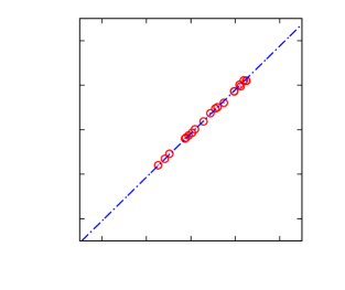
The details of the simulation are the same as they were described in Sec. 5.4, but now the initial gains of the layers were set randomly in the range 0.81.20.81.20.8-1.2. Only the first step in the list of Sec. 6.1 was performed. The extracted relative gains as function of the real values are shown in Fig. 21, for all the 16 layers used. While the gains are steadily smaller by about 1% (bias), they have an excellent relative precision.
0.60.811.21.40.60.811.21.4

Reconstructed relative gain

Real relative gain300-600 μ𝜇\mumRefer to caption
Figure 21: Reconstructed relative gains as function of the real values, shown for the 16 layers used in the detector simulation.

7 Conclusions

In this work a new analytical energy loss model for charged particles in silicon was introduced. It has few parameters and it is based on the recognition of a special connection between the distribution of the deposited energy and the most probable energy loss. Its use was demonstrated through several examples. With help of measured charge deposits in pixels or strips of hit clusters their position and energy can be estimated with better accuracy and much less bias. Deposits below threshold and saturated values are treated properly, resulting in a wider dynamic range. The model was successfully applied to track differential energy loss estimation and to detector gain calibration tasks, again showing a performance superior to standard methods.

Acknowledgements

The author wishes to thank to Sándor Hegyi, András László and Dániel Barna for helpful discussions. This work was supported by the Hungarian Scientific Research Fund with the National Office for Research and Technology (K 81614, H07-B 74296), and the Swiss National Science Foundation (128079).

References

  • [1] O. Ullaland, Update in particle identification, Nucl. Phys. Proc. Suppl. 125 (2003) 90–99. doi:10.1016/S0920-5632(03)90972-8.
  • [2] H. Yamamoto, dE/dx particle identification for collider detectorsarXiv:hep-ex/9912024.
  • [3] H. Bichsel, Straggling in thin silicon detectors, Rev. Mod. Phys. 60 (1988) 663–699. doi:10.1103/RevModPhys.60.663.
  • [4] K. Nakamura, et al., Review of particle physics, J.Phys.G G37 (2010) 075021. doi:10.1088/0954-3899/37/7A/075021.
  • [5] H. Bichsel, Inelastic electronic collision cross sections for Monte Carlo calculations, Nucl. Instrum. Meth. B52 (1990) 136. doi:10.1016/0168-583X\%2890\%2990581-E.
  • [6] H. Bichsel, A method to improve tracking and particle identification in TPCs and silicon detectors, Nucl. Instrum. Meth. A562 (2006) 154–197. doi:10.1016/j.nima.2006.03.009.
  • [7] M. Brigida, et al., A new Monte Carlo code for full simulation of silicon strip detectors, Nucl. Instrum. Meth. A533 (2004) 322–343. doi:10.1016/j.nima.2004.05.127.
  • [8] B. Efron, D. V. Hinkley, Assessing the accuracy of the maximum likelihood estimator: Observed versus expected Fisher Information, Biometrika 65 (1978) 454–487. doi:10.1093/biomet/65.3.457.
  • [9] Y. Allkofer, et al., Design and performance of the silicon sensors for the CMS barrel pixel detector, Nucl. Instrum. Meth. A584 (2008) 25–41. doi:10.1016/j.nima.2007.08.151.
  • [10] M. Swartz, D. Fehling, G. Giurgiu, P. Maksimovic, V. Chiochia, A new technique for the reconstruction, validation, and simulation of hits in the CMS pixel detector, PoS VERTEX2007 (2007) 035.
  • [11] W. H. Press, B. P. Flannery, S. A. Teukolsky, W. T. Vetterling, Numerical Recipes: The Art of Scientific Computing; 3rd ed., Cambridge Univ. Press, Cambridge, 2007.
  • [12] J. W. Lewis, Inversion of tridiagonal matrices, Numer. Math. 38 (1982) 333–345. doi:10.1007/BF01396436.
  • [13] E. D. Nering, A. W. Tucker, Linear programs and related problems, Academic Press Professional, Inc., San Diego, CA, USA, 1993.
  • [14] E. M. Gertz, S. J. Wright, Object-oriented software for quadratic programming, ACM Trans. Math. Softw. 29 (1) (2003) 58–81. doi:10.1145/641876.641880.
  • [15] R. Brun, F. Rademakers, ROOT: An object oriented data analysis framework, Nucl. Instrum. Meth. A389 (1997) 81–86. doi:10.1016/S0168-9002(97)00048-X.
  • [16] J. Shao, D. Tu, The jackknife and bootstrap, Springer series in statistics, Springer Verlag, 1995.
  • [17] R. C. Fernow, Introduction to experimental particle physics, Cambridge University Press, 1986, pages 253-255.
  • [18] C. Grupen, B. Shwartz, H. Spieler, Particle Detectors, 2nd Edition, Cambridge University Press, 2008, pages 278-280.
  • [19] J. Kiefer, Sequential minimax search for a maximum, Proc. Amer. Math. Soc. 4 (1953) 502–506. doi:10.2307/2032161.