Multifractal analyses of row sum signals of elementary cellular automata

Abstract

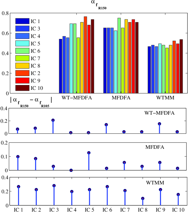
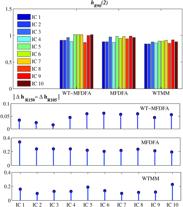
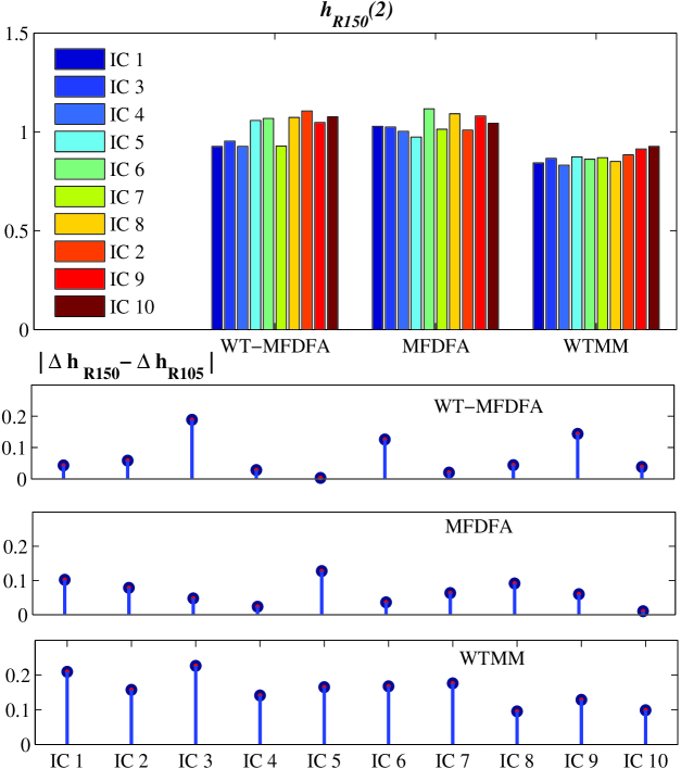
We first apply the WT-MFDFA, MFDFA, and WTMM multifractal methods to binomial multifractal time series of three different binomial parameters and find that the WTMM method indicates an enhanced difference between the fractal components than the known theoretical result. Next, we make use of the same methods for the time series of the row sum signals of the two complementary ECA pairs of rules (90,165) and (150,105) for ten initial conditions going from a single 1 in the central position up to a set of ten 1’s covering the ten central positions in the first row. Since the members of the pairs are actually similar from the statistical point of view, we can check which method is the most stable numerically by recording the differences provided by the methods between the two members of the pairs for various important quantities of the scaling analyses, such as the multifractal support, the most frequent Hölder exponent, and the Hurst exponent and considering as the better one the method that provides the minimum differences. According to this criterion, our results show that the MFDFA performs better than WT-MFDFA and WTMM in the case of the multifractal support, while for the other two scaling parameters the WT-MFDFA is the best. The employed set of initial conditions does not generate any specific trend in the values of the multifractal parameters.

I Introduction

Around 1975, Mandelbrot coined the term fractals to dynamical systems and objects with a hierarchy of structures that can be detected under changes of scales although related mathematical research on self-similar entities can be clearly traced back for at least two centuries and even some formulations in Euclid’s Elements can be judged to allude to self-affine properties. If the structures that appear at lesser scales are identical to the bigger ones the systems or objects are monofractals, while if the structures are different on various scales they can form the more general class of multifractals. It is then natural to think of multifractals as complex systems but with a complexity that can be still characterized in terms of scaling power laws whose exponents are known as scaling parameters. In addition, during the last two decades of the past century the paradigms of self-organized criticality and $1/f$ noise helped to make firm the idea of scaling laws of many hierarchical processes. Moreover, such scale-dependent structures can be measured only with measuring devices that are scale dependent themselves and their complexity can be characterized in terms of non-integer dimensions such as the Hausdorff dimension.

On the other hand, wavelet transforms (WT, briefly introduced in the Appendix) are pervading the analysis of multifractal processes since about two decades. It is well known that the spectra of Hausdorff dimensions are accessible from time series by a Legendre transform of the corresponding Hentschel-Procaccia (HP) spectra hp . Muzy and collaborators muzy1 proposed a dimension type characteristic based on the wavelet transform of a measure and in arne1 they demonstrated through several examples that the wavelet formalism yields the same spectra as the HP formalism and raised the conjecture that the equivalence of both formalisms should be valid in more general situations.

In this paper, we are interested in testing several multifractal numerical procedures to determine the scaling properties of the time series generated by the evolution of elementary cellular automata (ECA), originally introduced by von Neumann and Ulam during the 1960’s under the name of ‘cellular spaces’ as a way of modelling biological self-reproduction. ECA are a class of discrete dynamical systems since they evolve in discrete time steps. Willson will84 proved a long time ago that ECA are fractals by providing rigorous definitions and calculations of their fractal dimensions. In 2003, Sanchez s03 was the first to study the multifractality of some ECA evolution rules using the random walk approach of Peng et al Pengetal and together with Alonso-Sanz also examined the interplay between multifractality and memory effects sas . In 2005, Nagler and Claussen NC systematically computed the power spectra of the ECA time series of their row sum signals and found spectra of the type $1/f^{\alpha_{p}}$ with $\alpha_{p}=1.2$ and $\alpha_{p}=1.3$ but only for 10% of the 256 ECA rules.

This paper is organized as follows. ECA are introduced in the next section. A brief description of the numerical scaling methods is given in the third section. The multifractal scaling analyses of the ECA time series for the so-called row sum signals makes the body of the fourth section and last come the conclusions.

II Cellular Automata (CA)

During 1980s, because of the impetuous research of Wolfram cellular automata turned into a new scientific paradigm related to their ability to mimic through simple computed rules many natural processes W1 ; W2 . The state space of a CA of size $N$ is the set $\Omega=\mathbb{Z}^{N}_{k}$ of all sequences of $N$ cells that take values from $\mathbb{Z}_{k}=\{0,1,\ldots,k-1\}$, where its evolution is defined by the repeated iteration of an evolution operator $\mathcal{A}:\mathbb{Z}^{N}_{k}\to\mathbb{Z}^{N}_{k}$. In this paper, we consider only two-digit cells, $\mathbb{Z}_{2}=\{0,1\}$, regularly distributed in one space and one time dimensions, in which case the CA are called elementary. These ECA have only $2^{3}=8$ different first-order neighbourhoods $x_{i-1},x_{i},x_{i+1}$ which generates $2^{2^{3}}=256$ possible rules that are counted from 0 to 255. An automaton state $\underline{x}\in\mathbb{Z}^{\mathbb{Z}}_{2}$ has coordinates $(\underline{x})_{i}=x_{i}\in\mathbb{Z}_{2}$ with $i\in\mathbb{Z}$, and the automaton state at time $t\geq 0$ is denoted by $\underline{x}^{t}\in\mathbb{Z}^{\mathbb{Z}}_{2}$ and its evolution is defined iteratively by the rule $\underline{x}^{t+1}=\mathcal{A}(\underline{x}^{t})$. Starting from the initial state $\underline{x}^{0}$, the automaton generates the forward space-time pattern $\mathbf{x}\in\mathbb{Z}^{\mathbb{Z}\times\mathbb{N}}_{2}$ with state $(\mathbf{x})^{t}=\underline{x}^{t}=\mathcal{A}^{t}(\underline{x}^{0})$ reached at from $\underline{x}^{0}$ after $t\in\mathbb{N}$ time steps. $\mathbb{N}$ denotes the set of nonnegative integers.

One can see that the time, space, and states of this system take only discrete values. The first ECA that we consider here evolves according to the local rules

$$x_{i}^{t+1} \equiv\mathcal{A}_{90}(x_{i-1}^{t},x_{i}^{t},x_{i+1}^{t})=[x_{i-1}^{t}+x_{i+1}^{t}]{\rm mod}\ 2~{},$$

$$x_{i}^{t+1} \equiv\mathcal{A}_{165}(x_{i-1}^{t},x_{i}^{t},x_{i+1}^{t})=1-[x_{i-1}^{t}+x_{i+1}^{t}]\rm{mod}\ 2~{},$$

which correspond to the rule 90 and its complementary rule 165 described in the tabular form below:

Current neighbourhood pattern:	111	110	101	100	011	010	001	000
Rule result for central cell:    ${}^{90}_{165}$	${}^{0}_{1}$	${}^{1}_{0}$	${}^{0}_{1}$	${}^{1}_{0}$	${}^{1}_{0}$	${}^{0}_{1}$	${}^{1}_{0}$	${}^{0}_{1}$

The second row shows the future state of the cell if the cell itself and its left and right neighbors are in the arrangement shown in the first row. In fact, a rule is numbered by the unsigned decimal equivalent of the binary expression in the second row. For the second complementary pair considered here, the local rules are:

$$x_{i}^{t+1} \equiv\mathcal{A}_{150}(x_{i-1}^{t},x_{i}^{t},x_{i+1}^{t})=[x_{i-1}^{t}+x_{i}^{t}+x_{i+1}^{t}]{\rm mod}\ 2~{},$$

$$x_{i}^{t+1} \equiv\mathcal{A}_{105}(x_{i-1}^{t},x_{i}^{t},x_{i+1}^{t})=1-[x_{i-1}^{t}+x_{i}^{t}+x_{i+1}^{t}]\rm{mod}\ 2~{},$$

whereas their table form is the following one:

Current neighbourhood pattern:	111	110	101	100	011	010	001	000
Rule result for central cell:   $\displaystyle{{}^{150}_{105}}$	${}^{1}_{0}$	${}^{0}_{1}$	${}^{0}_{1}$	${}^{1}_{0}$	${}^{0}_{1}$	${}^{1}_{0}$	${}^{1}_{0}$	${}^{0}_{1}$

The uniform ECA are those for which the same rule is applied to update the cells as in this paper, otherwise the ECA are called non-uniform or hybrid.

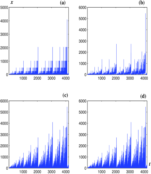
The time series that we consider in the case of the four ECA rules examined here belong to the row sum signals as used by Nagler and Claussen NC , i.e., the sums of the 1’s in each row (at each time step). Examples of the corresponding time series for the four ECA rules considered in this paper are displayed in Fig. 1.

It is also worth mentioning that the evolution rules of ECA are determined by two main factors: the rule and the initial conditions. For example, for our time series samples, in the case of the rule 90 with a single central 1 in the first row we have the first peak of amplitude $2^{11}$ at time (row) $2^{11}$, while the same peak is shifted two rows upwards if the initial condition is three 1’s in the central position. On the other hand, for the rule 150 with a central 1 in the first row there are no peaks of height $2^{11}$ but instead we have found peaks of height $2^{11}+1$ at the rows 1536, 2046, 2560, and so forth.

Figure 1: Time series of the row sum signal with a single 1 in the central position of the first row as initial condition corresponding to: (a) rule R90, (b) its complementary rule R165, (c) rule R150, and (d) its complementary rule R105. Only the first $2^{12}$ points are shown of the whole set of $2^{16}$ data points. Since the mean signals for the complementary rules are much higher than for the rules themselves showing also some specific trends we eliminated their contribution in the time series of the right column.

III Brief Description of the Multifractal Methods

In a previous work epl09 , we used the wavelet-transform detrended fluctuation analysis proposed by Manimaran mani , henceforth WT-MFDFA, to perform the multifractal analysis of three relevant ECA time series and found multifractal spectra estimates in quantitative agreement with the ones obtained with the multifractal detrended fluctuation analysis (MFDFA K03 ). However, recently, the literature abounds in comparison works related to the existing numerical methods for multifractal behaviour, which in fact try to establish their advantages and disadvantages one with respect to the others H11 . According to those works, the so-called wavelet leaders (WL), a scaling method that employs the coefficients of an orthogonal wavelet decomposition of the signal, seems to perform better than other competing methods, such as the WT modulus maxima (WTMM) and the MFDFA. Oświȩcimka et al. Osw processed synthesized data with WTMM and MFDFA and stated that the MFDFA provides a better estimation of singularity spectrum than WTMM. Jaffard et al. J05 claimed that also WL provides a better singularity spectrum than WTMM. In addition, a comparison study of Serrano and Figliola SF09 between WL and MFDFA favoured WL, although for short time series they recommend MFDFA to extract the multifractal spectrum. Regarding the estimation of the Hurst exponent, we note that in the review paper of Mielniczuk and Wojdyllo MW06 it is claimed that the properties of several variants of the DFA estimators differ greatly in their performance!

III.1 WT-MFDFA

An important class of wavelets are those with the vanishing moment property (see the Appendix) which directly helps to detrend the data. To reveal the MF properties of ECA one should separate the trend from fluctuations in the ECA time series. We decided to use the discrete wavelet method proposed by Manimaran et al. mani . This method exploits the fact that the low-pass version resembles the original data in an “averaged” manner in different resolutions. Instead of a polynomial fit, we consider the different versions of the low-pass coefficients to calculate the “local” trend. Let $x(t_{k})$ be a time series type of data, where $t_{k}=k\Delta t$ and $k=1,2,\ldots,~{}N$. Then the algorithm that we employ contains the following steps:

1. Determine the profile $Y(k)$ of the time series, which is the cumulative sum of the series from which the series mean value is subtracted, i.e., $Y(k)=\sum_{i=1}^{k}(x(t_{i})-\langle x\rangle)$.

2. Calculate the fast wavelet transform (FWT), i.e., the multilevel wavelet decomposition of the profile. For each level $m$, we get the fluctuations of the $Y(k)$ by subtracting the “local” trend of the $Y$ data, i.e., $\Delta Y(k;m)=Y(k)-\tilde{Y}(k;m)$, where $\tilde{Y}(k;m)$ is the reconstructed profile after removal of successive details coefficients at each level $m$. These fluctuations at level $m$ are subdivided into windows, i.e., into $M_{s}={\rm int}(N/s)$ non-overlapping segments of length $s$. This division is performed starting from both the beginning and the end of the fluctuations series (i.e., one has $2M_{s}$ segments). Next, one calculates the local variances associated to each window $\nu$

   $$F^{2}(\nu,s;m)={\rm var}\Delta Y((\nu-1)s+j;m)~{},\quad j=1,...,s~{},\quad\nu=1,...,2M_{s}~{}.$$ (1)

3. Calculate a $q$th order fluctuation function defined as

   $$F_{q}(s;m)=\left\{\frac{1}{2M_{s}}\sum_{\nu=1}^{2M_{s}}|F^{2}(\nu,s;m)|^{q/2}\right\}^{1/q}$$ (2)

   where $q\in\mathbb{Z}$ with $q\neq 0$. The diverging behaviour for $q\to 0$ can be avoided by using a logarithmic averaging $F_{0}(s;m)=\exp\left\{\frac{1}{2M_{s}}\sum_{\nu=1}^{2M_{s}}\ln|F^{2}(\nu,s;m)|\right\}$, see K02 .

If the fluctuation function $F_{q}(s;m)$ displays a power law scaling

$$F_{q}(s;m)\sim s^{h(q)},$$ (3)

then the analyzed time series has a fractal scaling behaviour. The exponent $h(q)$ is the generalized Hurst exponent since it depends on $q$, while the original Hurst exponent is $h(2)$. If $h(q)$ is constant for all $q$ then the time series is monofractal, otherwise it has a MF behavior. In the latter case, one can calculate various other MF scaling exponents, such as $\tau(q)$ and $f(\alpha)$ Halsey .

III.2 MFDFA

MFDFA is an algorithm developed in 2002 by Kantelhardt et al K02 , which differ from WT-MFDFA by the fact that it does not make use of WT for detrending. In fact the origin of both procedures is the conventional detrended fluctuation analysis of Peng et al Pengetal . Again the data to be considered are profiles of the signals, which are divided into non-overlapping segments both from the beginning and from the end of the set of data getting therefore $2N_{s}$ segments altogether. In each of these segments the local trend is calculated by a least square fit of the series. Then one calculates the variance $F^{2}(s,\nu)$ for each segment $\nu$ with respect to the fitting line $y_{\nu}$ in each segment $\nu$. Finally, an average over all segments is performed leading to the $q$–th order fluctuation function similar to (2)

$$F_{q}(s)=\left\{\frac{1}{2N_{s}}\sum_{\nu=1}^{2N_{s}}|F^{2}(\nu,s)|^{q/2}\right\}^{1/q}~{}.$$ (4)

III.3 WTMM

In the presence of an isolated singularity in the data at a particular point $t_{0}$, the scaling behavior of the wavelet coefficients (see equation (11) in the appendix) is described by the Hölder exponent $\alpha(t_{0})$ as

$$W_{x}(a,t_{0})\sim a^{\alpha(t_{0})+1/2},$$ (5)

in the limit $a\to 0^{+}$. To characterize the singular behavior of functions, it is sufficient to consider the values and positions of the Wavelet Transform Modulus Maxima (WTMM) mallat-huang defined as points $(a_{0},b_{0})$ on the scale-position plane, $(a,b)$, where $|W_{x}(a_{0},b)|$ is locally maximum for $b$ in the neighborhood of $b_{0}$. These maxima are located along curves in the plane $(a,b)$. However, the relationship (5) in some cases is not appropriated to describe distribution functions with non-isolated singularities. The wavelet multifractal formalism may characterize fractal objects which cannot be completely described using a single fractal dimension. According to Bacry et al. arne1 , an “optimal” partition function ${\mathcal{Z}}_{q}(x,a)$ can be defined in terms of the WTMM. They consider the set of modulus maxima at a scale $a$ as a covering of the singular support of $x$ with wavelets of scale $a$. The partition function ${\mathcal{Z}}_{q}$ measures the sum of all wavelet modulus maxima at a power $q$ as follows

$${\mathcal{Z}}_{q}(x,a)=\sum_{p}|W_{x}(a,b_{p}(a))|^{q},$$ (6)

where $\{b_{p}(a)\}_{p\in\mathbb{Z}}$ is the position of all local maxima of $|W_{x}(a,b)|$ at a fixed scale $a$. This partition function is very close to the definition of the partition function introduced in Halsey . It can be inferred from (6) that for $q>0$ the most pronounced modulus maxima will prevail, whereas for $q<0$ the lower ones will survive. For each $q\in\mathbb{R}$, the partition function is related to its scaling exponent $\tau(q)$ in the following way ${\mathcal{Z}}_{q}(x,a)\sim a^{\tau(q)}$. A linear behavior of $\tau(q)$ indicates monofractality whereas nonlinear behavior suggests that a signal is a multifractal. A fundamental result in the (wavelet) multifractal formalism states that the singularity (Hölder) spectrum $f(\alpha)$ of the signal $x(t)$ is the Legendre transform of $\tau(q)$, i.e.,

$$\alpha=\frac{d\tau(q)}{dq},\qquad\text{and}\qquad f(\alpha)=q\alpha-\tau(q).$$ (7)

The Hölder spectrum of dimensions $f(\alpha)$ is a non-negative convex function that is supported on the closed interval $[\alpha_{\text{min}},\alpha_{\text{max}}]$, which is interpreted as the Hausdorff fractal dimension of the subset of data characterized by the Hölder exponent $\alpha$ Salo1 . The most “frequent” singularity, which corresponds to the maximum of $f(\alpha)$, occurs for the value of $\alpha(q=0)$, whereas the boundary values of the support, $\alpha_{\text{min}}$ for $q>0$ and $\alpha_{\text{max}}$ for $q<0$, correspond to the strongest and weakest singularity, respectively.

The analyzing wavelets which are used most frequently are the successive derivatives of the Gaussian function

$$\psi^{(n)}(t):=\frac{d^{n}}{dt^{n}}\left(\exp(-t^{2}/2)\right),\qquad n\in\mathbb{Z}^{+},$$ (8)

because they are well localized both in space and frequency, and they remove the trends of the signal that can be approximated by polynomials up to $(n-1)$th order. In particular, our analyses were carried out with the Mexican hat wavelet $\psi^{(2)}(t)$.

IV Data analyses

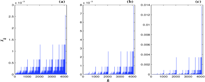
In order to illustrate the efficiency and the fitting properties of the three procedures, we first carry out the analysis of the binomial multifractal time series, whose scaling parameters are analytically known K02 ; Feder . The binomial multifractal time series are series of $N=2^{n_{\textrm{max}}}$ numbers $x_{k}$, with $k=1,\ldots,N$, defined by

$$x_{k}=c^{n(k-1)}(1-c)^{n_{\textrm{max}}-n(k-1)}.$$ (9)

where $0.5<c<1$ is a parameter and $n(k)$ is the number of digits equal to 1 in the binary representation of the index $k$. Examples of binomial time series $x_{k}$ for three values of the parameter $c$ are given in Fig. (2).

Figure 2: Binomial time series $x_{k}$ for the binomial model (9) of parameters $c=2/3$, $3/4$, and $4/5$ from left to right, respectively. We have used $n_{\rm max}=13$ but only the first $2^{12}$ data are shown.

The binomial multifractal exponents $h(q)$ and $\tau(q)$ can be calculated in closed forms

$$h(q)=\frac{1}{q}-\frac{\ln[c^{q}+(1-c)^{q}]}{q\ln 2},\qquad\tau(q)=-\frac{\ln[c^{q}+(1-c)^{q}]}{\ln 2}.$$ (10)

Figure 3 shows the multifractal singularity spectrum $f(\alpha)$, the generalized Hurst exponent, and the $\tau$ exponent for three values of the binomial parameter $c$.

Figure 3: The singularity spectrum $f(\alpha)$, the generalized Hurst exponent, and the $\tau$ exponent for the binomial multifractal model of parameters $c=2/3$ (left column), $c=3/4$ (middle column), and $c=4/5$ (right column). $\rm M1$ corresponds to WT-MFDFA, $\rm M2$ to MFDFA, and $\rm M3$ to WTMM, while $\rm Th$ corresponds to the theoretical binomial formulas for the same parameters.

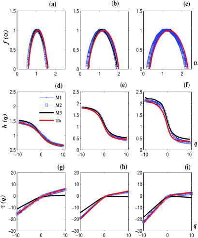
A direct inspection of the binomial multifractal plots shows that the numerical differences between the three methods are not significant in the case of the singularity spectra and the generalized Hurst exponent, although the WT-MFDFA and MFDFA are closer to the theoretical curves than the WTMM method. In the case of the $\tau$ exponent, the WTMM clearly indicates a more pronounced multifractality than the theoretical one, while the first two methods are again very close to the theoretical curve. We have checked that the high $|q|$ discrepancies of the WTMM $\tau$ exponent stay almost constant at least for sample sizes up to $2^{16}$ data but we do not rule out the WTMM procedure because as we said the singularity spectra and the Hurst exponent obtained by this method do not appear to be different from the binomial theoretical results in a relevant manner.

We proceed with the comparison study among the three scaling approaches, namely the WT-MFDFA, MFDFA, and WTMM analyses, for the time series of the row sum signals of two pairs of complementary ECA rules (90, 165) and (105,150) with the goal of providing further evidence of their multifractal nature and also to check the performance of the three scaling methods. The idea behind the latter test is simple. Since the rules in the pairs are complementary in the sense that their transition rates fulfill $f_{105}=1-f_{150}$ and $f_{90}=1-f_{165}$ they should not differ statistically for samples of reasonable sizes and should provide quite similar results. Therefore, the most reliable scaling method is the one which gives the smallest fluctuations in the differences of the scaling parameters between the two members of any complementary ECA pair.

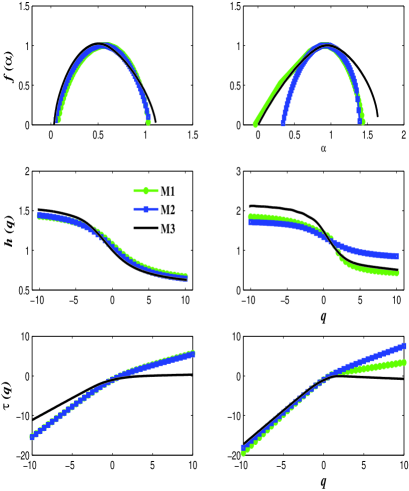
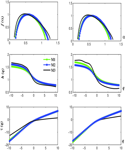
The main multifractal quantities are displayed in Fig. 4 for the first ECA pair and in Fig. 5 for the second one. As in the binomial case, the simple inspection of the plots indicates the following features. WT-MFDFA is closer to WTMM on the left wing of the singularity parabola ($\alpha<\alpha_{\rm max}$), whereas it is closer to the MFDFA on the right wing ($\alpha>\alpha_{\rm max}$). In the case of $h(q)$, WT-MFDFA is closer to MFDFA at negative $q$s but closer to WTMM at positive $q$s. Finally, for $\tau(q)$ WT-MFDFA is always closer to MFDFA; in fact, for rule 90 the results of the two methods are almost identical. At the same time, WT-MFDFA indicates a less pronounced difference between the fractal components than MFDFA and WTMM, as taken in this order. Similar results are obtained for the second pair although these tendencies are less pronounced.

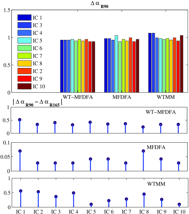
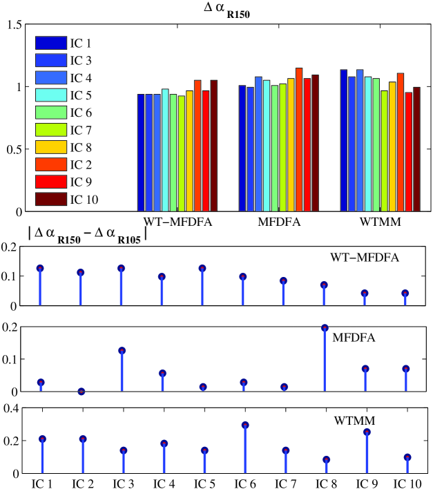
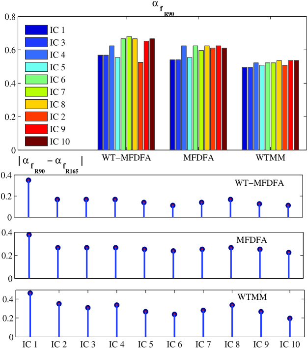
We merely use the WT-MFDFA here rather than WL because we employed it in our previous paper epl09 and in fact both procedures are based on the coefficients of an orthogonal wavelet decomposition. Our results for the extension (support) of the multifractality, the most frequent Hölder exponent, and the Hurst exponent are presented graphically in Figures 6, 8, and 10, respectively, for the ECA pair (90,165) and in Figures 7, 9, and 11, for the pair (150,105) as three groups of ten histograms corresponding to the three methods and ten initial conditions of centered activity type, i.e., with symmetrically distributed 1’s around the central position in the first row. As commented in the captions, the plots indicate that in the case of the multifractal support, the MFDFA gives smaller differences between the two complementary rules than WT-MFDFA and WTMM, while for the other two scaling parameters the WT-MFDFA is the best from this point of view. We also mention that the arguments of Huang and collaborators H11 against representing a continuous signal through a discrete WT do not apply to our data because the CA signals are naturally discrete.

Figure 4: The singularity spectrum $f(\alpha)$, the generalized Hurst exponent, and the $\tau$ exponent for the rule pair (90–165) for the three multifractal methods employed here.

Figure 5: The singularity spectrum $f(\alpha)$, the generalized Hurst exponent, and the $\tau$ exponent for the rule pair (150–105) for the three multifractal methods as above.

V Conclusions

In conclusion, we provided here a strong confirmation of our previous results epl09 that the implementation of the discrete WT in the MFDFA method leads to the WT-MFDFA as a very acceptable algorithm to obtain the multifractal ECA parameters with much less computational cost and better accuracy. We also found that there is no apparent trend in the results depending on an extended set of initial conditions represented by an extended centered initial activity in the CA terminology. Since we used complementary automaton rules, which are statistically identical we could compare the numerical results of the WT-MFDFA, MFDFA, and WTMM procedures. According to the criterion of minimum differences in the scaling quantities for statistically identical data, it appears that the MFDFA performs better than WT-MFDFA and WTMM in the case of the multifractal support, while for the most frequent Hölder exponent and the Hurst exponent the WT-MFDFA is the best. The same numerical techniques have been tested for the analytically known case of binomial multifractal time series for three binomial parameters with the result that WT-MFDFA and MFDFA reproduce very closely the theoretical values of the multifractal quantities. This can be interpreting as compelling evidence that the latter numerical methods are reliable tools to calculate the multifractal properties.

Figure 6: Rule 90 ECA: The multifractal support $\Delta\alpha$ in the case of the row sum signal of a sequence of $2^{13}$ time steps with the ten initial conditions as explained in the text. There are no significant differences in the case of the three scaling methods that we tested. In the lower three plots, the differences $|\Delta\alpha_{R90}-\Delta\alpha_{R165}|$ between the multifractal supports of the two complementary rules for each scaling methods are displayed. The MFDFA procedure gives differences less than 0.08 for the ten tested initial conditions, much better than WT-MFDFA and WTMM.

Figure 7: Rule 150 ECA: The multifractal support $\Delta\alpha$ in the case of the row sum signal of a sequence of $2^{13}$ time steps with the same initial conditions. There are no significant differences in the case of the three scaling methods that we tested. In the lower three plots, the differences $|\Delta\alpha_{R150}-\Delta\alpha_{R105}|$ between the multifractal supports of the two complementary rules for each scaling methods are displayed. Although WT-MFA and WTMM performs better for this complementary pair than for the other one, the MFDFA procedure still provides less differences.

Figure 8: Rule 90 ECA: The most frequent Hölder exponent $\alpha_{f}$ obtained with WT-MFA, MFDFA, and WTMM for the ten initial conditions. The lower three plots display the difference $|\alpha_{f_{R90}}-\alpha_{f_{R165}}|$. In this case, the WT-MFDFA works better.

Figure 9: Rule 150 ECA: The most frequent Hölder exponent $\alpha_{f}$ obtained with WT-MFA, MFDFA, and WTMM for the same initial conditions. The lower three plots display the difference $|\alpha_{f_{R150}}-\alpha_{f_{R105}}|$. The WT-MFDFA works better again.

Figure 10: Rule 90 ECA: The Hurst exponent $h_{R90}(2)$ and the differences with respect to the complementary rule for the three scaling methods. One can see that WT-MFDFA still performs better.

Figure 11: Rule 150 ECA: The same as in the previous figure. WT-MFDFA is still better globally.

Appendix: Wavelet theory

The wavelet transform (WT for short) of a signal $x(t)$ is given by

$$W_{x}(a,b)=\frac{1}{\sqrt{a}}\int_{-\infty}^{\infty}x(t)\bar{\psi}\left(\frac{t-b}{a}\right)dt,$$ (11)

where $\psi$ is the analyzing wavelet, $b\in\mathbb{R}$ is a translation parameter, whereas $a\in\mathbb{R}^{+}~{}(a\neq 0)$ is a dilation or scale parameter, and the bar symbol denotes complex conjugation.

One fundamental property that is required to analyze singular behavior is that $\psi(t)$ has enough vanishing moments arne1 ; Mallat . A wavelet is said to have $n$ vanishing moments if and only if it satisfies

$$\int_{-\infty}^{\infty}t^{k}\psi(t)dt =0,\quad\text{for ~{} $k=0,1,\ldots,n-1$,}\,\quad\text{and}\quad\int_{-\infty}^{\infty}t^{n}\psi(t)dt\neq 0~{}.$$ (12)

This means that a wavelet with $n$ vanishing moments is orthogonal to all polynomials up to order $n-1$. Thus, the wavelet transform of $x(t)$ performed by means of a wavelet $\psi(t)$ with $n$ vanishing moments is nothing but a “smoothed version” of the $n$–th derivative of $s(t)$ on various scales.

Since in general the majority of data are represented by a finite number of values, we consider the orthogonal (discrete) wavelet case in which the wavelets are associated to orthonormal bases of $L^{2}(\mathbb{R})$. First, a discrete grid is established for the dilation and translation parameters such that wavelet function $\psi(t)$, and its associated scaling function $\varphi(t)$ Mallat ; Ingrid can be expressed in the form

$$\varphi_{m,n}(t)=2^{m/2}\varphi(2^{m}t-n),\qquad\psi_{m,n}(t)=2^{m/2}\psi(2^{m}t-n),\quad m,n\in\mathbb{Z}$$ (13)

with $m$ and $n$ denoting the dilation and translation indices, respectively.

Within this framework, one can write the expansion of an arbitrary signal $x(t)$ in an orthonormal wavelet basis as follows

$$x(t)=\sum_{n}\left(a_{m_{0},n}\varphi_{m_{0},n}(t)+\sum_{m=m_{0}}^{M-1}d_{m,n}\psi_{m,n}(t)\right),$$ (14)

where the scaling or approximation coefficients $a_{m,n}$ and the wavelet coefficients $d_{m,n}$ are given by

$$a_{m,n}=\int x(t)\varphi_{m,n}(t)dt,\qquad d_{m,n}=\int x(t)\psi_{m,n}(t)dt.$$ (15)

In this context, a computationally efficient method to compute (15) was developed by Mallat Mallat under the name of multi-resolution analysis (MRA). The MRA approach provides a general method for constructing orthogonal wavelet basis and leads to the implementation of the fast wavelet transform (FWT). A multi-resolution decomposition of a signal is based on successive decomposition into a series of approximations and details, which become increasingly coarse. The FWT calculates the scaling and wavelet coefficients at scale $m$ from the scaling coefficients at the next finer scale $m+1$ using

$$a_{m,n} =\sum_{k}h[k-2n]a_{m+1,k},$$ (16)

$$d_{m,n} =\sum_{k}g[k-2n]a_{m+1,k},$$ (17)

where $h[n]$ and $g[n]$ are typically called low pass and high pass filters in the associated analysis filter bank. In fact, the signals $a_{m,n}$ and $d_{m,n}$ are the convolutions of $a_{m+1,n}$ with the filters $h[n]$ and $g[n]$ followed by a downsampling of factor 2 Mallat , respectively.

Conversely, a reconstruction of the original scaling coefficients $a_{m+1,n}$ can be made from the following combination of the scaling and wavelet coefficients at a coarse scale

$$a_{m+1,n}=\sum_{k}\left(h[2k-n]a_{m,k}+g[2k-n]d_{m,k}\right)~{}.$$ (18)

It corresponds to the synthesis filter bank. This part can be viewed as the discrete convolutions between the upsampled signal $a_{m,l}$ and the filters $h[n]$ and $g[n]$, that is, following an upsampling of factor 2 the convolutions between the upsampled signal and the filters $h[n]$ and $g[n]$ are calculated.

References

- (1) H.G.E. Hentschel, I. Procaccia, Physica D 8 (1983) 435.
- (2) J.F. Muzy, E. Bacry, A. Arneodo, Phys. Rev. Lett. 67 (1991) 3515.
- (3) E. Bacry, J.F. Muzy, A. Arneodo, J. Stat. Phys. 70 (1993) 635.
- (4) S.J. Willson, Physica D 10 (1984) 69.
- (5) J.R. Sanchez, Int. J. Mod. Phys. C 14 (2003) 695.
- (6) C.-K. Peng, S.V. Buldyrev, A.L. Goldberger, S. Havlin, F. Sciortino, M. Simons, H.E. Stanley, Nature 35 (1992) 168.
- (7) J.R. Sanchez, R. Alonso-Sanz, Int. J. Mod. Phys. C 15 (2004) 1461.
- (8) J. Nagler, J.C. Clausen, Phys. Rev. E 71 (2005) 067103.
- (9) S. Wolfram, Cellular Automata and Complexity: Collected Papers (Westview Press, Boulder) 1994.
- (10) S. Wolfram, A New Kind of Science (Wolfram Media Inc., Champaign) 2002.
- (11) J.S. Murguía, J.E. Pérez-Terrazas, H.C. Rosu, Europhys. Lett 87 (2009) 28003.
- (12) P. Manimaran, P.K. Panigrahi, J.C. Parikh, Phys. Rev. E 72 (2005) 046120.
- (13) J.W. Kantelhardt, D. Rybski, S.A. Zschiegner, P. Braun, E. Koscielny-Bunde, V. Livina, S. Havlin, A. Bunde, Physica A 330 (2003) 240.
- (14) Y.X. Huang, F.G. Schmitt, J.-P. Hermand, Y. Gagne, Z.M. Lu, Y.L. Liu, Phys. Rev. E 84 (2011) 016208.
- (15) P. Oświȩcimka, J. Kwapién, S. Drozdz, Phys. Rev. E 74 (2006) 016103.
- (16) S. Jaffard, B. Lashermes, P. Abry, in Wavelet Analysis and Applications, (Birkhäuser Verlag, Basel) 2006.
- (17) E. Serrano, A. Figliola, Physica A 388 (2009) 2793.
- (18) J. Mielniczuk, P. Wojdyllo, Comp. Statistics & Data Analysis 51 (2007) 4510.
- (19) J.W. Kantelhardt, S.A. Zschinegner, E. Koscielny-Bunde, S. Havlin, A. Bunde, H.E. Stanley, Physica A 316 (2002) 87.
- (20) J. Feder, Appendix B in Fractals (Plenum Press, New York) 1998.
- (21) T.C. Halsey, M.H. Jensen, L.P. Kadanoff, I. Procaccia, B.I. Shraiman, Phys. Rev. A 33 (1986) 1141.
- (22) S. Mallat, W.L. Hwang, IEEE Trans. Inform. Theory 38 (2) (1992) 617 643.
- (23) J.S. Murguía, J. Urías, Chaos 11 (2001) 858 863.
- (24) S. Mallat, A Wavelet Tour of Signal Processing (Academic Press, New York) 1999.
- (25) I. Daubechies, Ten Lectures on Wavelets (SIAM, Philadelphia, PA) 1992.