Galaxy and Mass Assembly (GAMA): galaxy luminosity functions
Abstract
Galaxy and Mass Assembly (GAMA) is a project to study galaxy formation and evolution, combining imaging data from ultraviolet to radio with spectroscopic data from the AAOmega spectrograph on the Anglo-Australian Telescope. Using data from phase 1 of GAMA, taken over three observing seasons, and correcting for various minor sources of incompleteness, we calculate galaxy luminosity functions (LFs) and their evolution in the passbands.
At low redshift, , we find that blue galaxies, defined according to a magnitude-dependent but non-evolving colour cut, are reasonably well fitted over a range of more than ten magnitudes by simple Schechter functions in all bands. Red galaxies, and the combined blue-plus-red sample, require double power-law Schechter functions to fit a dip in their LF faintwards of the characteristic magnitude before a steepening faint end. This upturn is at least partly due to dust-reddened disc galaxies.
We measure evolution of the galaxy LF over the redshift range both by using a parametric fit and by measuring binned LFs in redshift slices. The characteristic luminosity is found to increase with redshift in all bands, with red galaxies showing stronger luminosity evolution than blue galaxies. The comoving number density of blue galaxies increases with redshift, while that of red galaxies decreases, consistent with prevailing movement from blue cloud to red sequence. As well as being more numerous at higher redshift, blue galaxies also dominate the overall luminosity density beyond redshifts . At lower redshifts, the luminosity density is dominated by red galaxies in the bands, by blue galaxies in and .
keywords:
galaxies: evolution — galaxies: luminosity function, mass function — galaxies: statistics.1 Introduction
Measurements of the galaxy luminosity function (LF) and its evolution provide important constraints on theories of galaxy formation and evolution, (see e.g. Benson et al. 2003). It is currently believed that galaxies formed hierarchically from the merger of sub-clumps. Looking back in time with increasing redshift, the star formation rate appears to peak at redshift , above which it plateaus and slowly declines towards (Cole et al., 2000; Hopkins, 2004; Hopkins & Beacom, 2006; Yuksel et al., 2008; Kistler et al., 2009). Since , galaxies are thought to have evolved mostly passively as their stellar populations age, with occasional activity triggered by accretion and interactions with other galaxies. Noeske et al. (2007) have suggested that the first major burst of star formation is delayed to later times for low mass galaxies, contributing to the downsizing phenomenon.
There has long been a discrepancy between the measured number density of low-luminosity galaxies (the ‘faint end’ of the LF) and predictions from cold dark matter (CDM) hierarchical simulations, in the sense that fewer low-luminosity galaxies than predicted by most models are observed (Trentham & Tully, 2002). Of course, interpretation of these simulation results is subject to uncertainties in the baryon physics. In particular, more effective feedback in low mass halos might act to suppress the faint end of the LF. However, it is also possible that many surveys have underestimated the number of dwarf galaxies due to the correlation between luminosity and surface brightness which makes them hard to detect (Driver, 1999; Cross & Driver, 2002; Cameron & Driver, 2007, 2009). Geller et al. (2011) have recently demonstrated that the LF faint-end slope steepens with decreasing surface brightness.
Galaxy LFs have previously been measured in the bands from the Sloan Digital Sky Survey (SDSS, York et al., 2000) by Blanton et al. (2003b), Loveday (2004), Blanton et al. (2005b), Montero-Dorta & Prada (2009), and Hill et al. (2010). Blanton et al. (2003b) analysed a sample of 147,986 galaxies, roughly equivalent to SDSS Data Release 1 (DR1, Abazajian et al., 2003). They fit the LF with a series of overlapping Gaussian functions, allowing the amplitude of each Gaussian to vary, along with two parameters and describing, respectively, luminosity and density evolution. They maximized the joint likelihood of absolute magnitude and redshift, rather than the likelihood of absolute magnitude given redshift, making this estimator more sensitive to evolution, as well as to density fluctuations due to large-scale structure. They found luminosity densities at to increase systematically with effective wavelength of survey band, and for luminosity evolution to decline systematically with wavelength. Allowing for LF evolution enabled reconciliation of previously discrepant luminosity densities obtained from SDSS commissioning data (Blanton et al., 2001) and the Two-degree field Galaxy Redshift Survey (Folkes et al., 1999; Norberg et al., 2002).
Loveday (2004) measured the -band LF in redshift slices from SDSS DR1 and found that the comoving number density of galaxies brighter than mag was a factor higher at redshift than today, due to luminosity and/or density evolution.
Blanton et al. (2005b) focused on the faint end of the LF of low-redshift galaxies from SDSS DR2 (Abazajian et al., 2004), and found that a double-power-law Schechter function was required to fit an upturn in the LF at mag with faint-end slope after correcting for low surface-brightness incompleteness.
Montero-Dorta & Prada (2009) have analysed SDSS DR6 (Adelman-McCarthy et al., 2008) which is roughly five times larger than the sample analysed by Blanton et al. (2003b). Their results are generally consistent with those of Blanton et al., although they do point out a bright-end excess above Schechter function fits, particularly in the and bands, due primarily to active galactic nuclei (AGNs). A bright-end excess above a best-fitting Schechter function has also been observed in near-IR passbands by Jones et al. (2006).
Hill et al. (2010) analysed combined datasets from the Millennium Galaxy Catalogue (Liske et al., 2003), SDSS and the UKIDSS Large Area Survey (Lawrence et al., 2007) over a common volume of within redshift to obtain LFs in the bands. They found that LFs in all bands were reasonably well fitted by Schechter functions, apart from tentative upturns at the faint ends of the - and -band LFs. Hill et al. provided the first homogeneous measurement of the luminosity density (LD) over the optical–near-IR regimes, finding a smooth spectral energy distribution (SED).
Here we present an estimate of galaxy LFs from the Galaxy and Mass Assembly (GAMA, Driver et al., 2009, 2011) survey. GAMA provides an ideal sample with which to constrain the galaxy LF at low to moderate redshifts due to its combination of moderately deep spectroscopic magnitude limit ( or ) and wide-area sky coverage (three deg2 regions).
We describe the input galaxy sample and incompleteness, velocity and -corrections in Section 2. Our LF estimation procedure is described in Section 3 and tested using simulations in Appendix A. We present our results and a discussion of luminosity and density evolution in Section 4, with our conclusions summarized in Section 5.
Unless otherwise stated, we assume a Hubble constant of km/s/Mpc and an cosmology in calculating distances, co-moving volumes and luminosities.
2 Data and observations
2.1 Input catalogue
The input catalogue for GAMA is described in detail by Baldry et al. (2010). In brief, it consists of three deg2 regions centred approximately on the equator and at right ascensions of 9, 12 and 14.5 hours. These fields are known as G09, G12 and G15 respectively. Primary galaxy targets were selected from Data Release 6 (DR6, Adelman-McCarthy et al., 2008) of the Sloan Digital Sky Survey (SDSS, York et al., 2000) to extinction-corrected, Petrosian magnitude limits of mag in the G09 and G15 fields and mag in the G12 field.
We require Petrosian and model magnitudes and their errors in all five SDSS passbands in order to determine -corrections (Section 2.5), and so we match objects in the GAMA team catalogue TilingCatv16 to objects in the SDSS DR6 PhotoObj table on SDSS ObjID using the SDSS CasJobs111http://casjobs.sdss.org/CasJobs/ service. We use only objects with GAMA survey_class in order to exclude additional filler targets from the sample. We exclude objects, which, upon visual inspection, showed no evidence of galaxy light, were not the main part of a deblended galaxy, or had compromised photometry (vis_class = 2, 3 or 4 respectively). See Baldry et al. (2010) for further details of these target flags and Section 2.7 for a discussion of additional visual inspection of extreme luminosity objects.
In estimating LFs, we use Petrosian magnitudes corrected for Galactic extinction according to the dust maps of Schlegel, Finkbeiner, & Davis (1998). We make no attempt here to correct for intrinsic dust extinction within each galaxy, as was done by Driver et al. (2007), nor to extrapolate the Petrosian magnitudes to total, as done, for example, by Graham et al. (2005) and Hill et al. (2011). These systematic corrections to SDSS photometry, much more significant than any small random errors, will be considered in a subsequent paper.
An exception to our use of Petrosian magnitudes is for -band data, where we instead use a pseudo-Petrosian magnitude defined by
| (1) |
The reason for this is that the Petrosian -band quantities are noisy and suffer from systematic sky-subtraction errors (Baldry et al., 2005). The pseudo-Petrosian -band magnitude defined above, (using the SDSS band since it has highest signal-to-noise), and referred to as by Baldry et al. (2005), is much better behaved at faint magnitudes.
For colour selection (see Section 2.6), we use SDSS model magnitudes in defining colour, as recommended by the SDSS website222http://www.sdss.org/dr7/algorithms/photometry.html.
2.2 Spectroscopic observations
GAMA spectroscopic observations are described in the first GAMA data release paper (Driver et al., 2011). Observations for the GAMA Phase 1 campaign were made over 100 nights between 2008 February and 2010 May, comprising 493 overlapping two-degree fields. Redshifts were assigned in a semi-automated fashion by the observers at the telescope. A subsequent re-redshifting exercise (Liske et al. in prep.) was used to assign a normalised quality to each redshift, according to each particular observer and their assigned quality . Here we use reliable () redshifts from all three years of the GAMA Phase 1 campaign. In addition to pre-existing redshifts and those obtained with the Anglo-Australian Telescope, twenty redshifts of brighter galaxies were obtained with the Liverpool Telescope. The GAMA-II campaign, extending the survey to additional southern fields, began in 2011, but only GAMA-I redshifts are used here.
2.3 Completeness
Although GAMA has a very high spectroscopic completeness ( per cent; Driver et al. 2011), the small level of incompleteness is likely to preferentially affect low surface brightness, low luminosity galaxies, or galaxies lacking distinctive spectral features. We have identified three sources of incompleteness that potentially affect the survey: the completeness of the input catalogue (imaging completeness), completeness of the targets for which spectra have been obtained (target completeness) and the success rate of obtaining spectroscopic redshifts (spectroscopic success rate). These three sources of incompleteness, and how we correct for them, are now considered in turn.
2.3.1 Imaging completeness
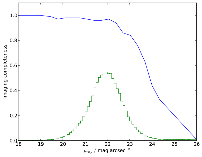
Imaging completeness has been estimated for the SDSS main galaxy sample by Blanton et al. (2005b), who passed fake galaxy images through the SDSS photometric pipeline. Blanton et al. found that imaging completeness is nearly independent of apparent magnitude (at least down to mag), depending mostly on -band half-light surface brightness, (their Fig. 2). Thus, while GAMA goes about 2 mag fainter than the SDSS main galaxy sample, the Blanton et al. imaging completeness should still be approximately applicable. We have used their imaging completeness estimates modified in the following ways333An alternative way of estimating imaging completeness is to determine what fraction of galaxies detected in the much deeper co-added data from SDSS Stripe 82 (Abazajian et al., 2009) are detected in regular, single-epoch SDSS imaging. However, one needs to allow for the large number of bright star or noise images misclassified as low surface-brightness galaxies in the SDSS co-added catalogue, and so this approach was abandoned. It will be re-explored once high-quality VST KIDS imaging of the GAMA regions becomes available.:
-
1.
Blanton et al. determine imaging completeness over the surface brightness range mag arcsec-2. Extrapolating their completeness as faint as mag arcsec-2 results in negative completeness values. We therefore arbitrarily assume 1 per cent imaging completeness at mag arcsec-2 and linearly interpolate from the faintest tabulated Blanton et al. completeness point at (, ) = (24.34, 0.33).
-
2.
The Blanton et al. imaging completeness decreases at the bright end, mag arcsec-2, due to a lower angular size limit of arcsec and a star-galaxy separation criterion for the SDSS main galaxy sample which excludes some compact, high surface-brightness (HSB) galaxies. GAMA target selection uses a far less stringent , backed up by colour selection, and so is much more complete in HSB galaxies. We therefore omit the Blanton et al. completeness points at mag arcsec-2 and instead assume 100 per cent completeness at mag arcsec-2 and brighter.
Our revised imaging completeness curve, along with a histogram of values for GAMA galaxies, is given in Fig.1.
2.3.2 Target completeness
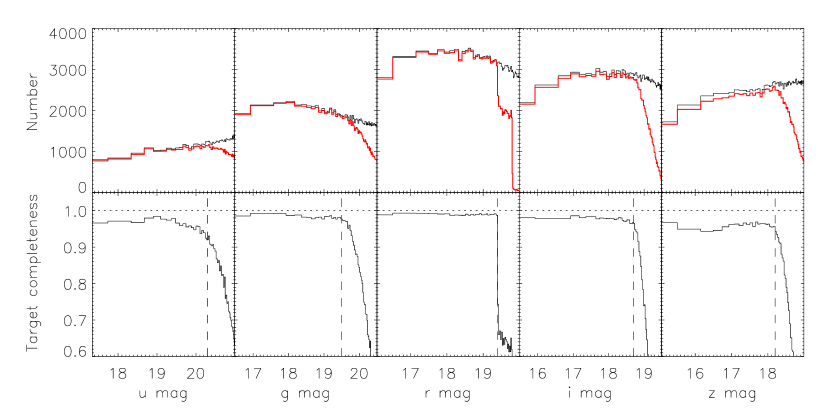
Target completeness in the band may be assessed relative to the GAMA tiling catalogue, which contains all galaxies to mag in the GAMA regions. In the bands, however, there is no well-defined magnitude limit. We therefore re-implement the GAMA target selection criteria detailed by Baldry et al. (2010) on samples of objects selected from the SDSS DR6 photoObj table. We replace the Baldry et al. (2010) magnitude limits (their equation 6) with the following: , , , or .
Target completeness in each band is then simply defined as the fraction of target galaxies that have been spectroscopically observed, either by GAMA or by another redshift survey, as a function of apparent magnitude in that band. This is shown in Fig. 2, where we have used magnitude bins which are equally spaced in . This binning is chosen to give a roughly equal number of galaxies per bin, thus avoiding large Poisson uncertainties at bright magnitudes. In the band, target completeness is around 98-99 per cent brighter than mag corresponding to the magnitude limit of the GAMA G09 and G15 fields.
In the other four bands, the drop in completeness at faint magnitudes is more gradual due to the spread in galaxy colours. Magnitude limits in each band are set to the faintest magnitude at which target completeness is at least 92 per cent ( band) or where completeness starts to drop rapidly. These magnitude limits are 20.3, 19.5, 19.4, 18.7, 18.2 in respectively and are indicated by the vertical dashed lines in Fig. 2.
An alternative approach to estimating the LF in bands other than that of target selection is to perform a multivariate LF, e.g. Loveday (2000), or to use a estimator where is calculated using the selection-band magnitude, e.g. Smith, Loveday & Cross (2009). While using more data, these estimators suffer from a colour bias as one approaches the sample flux limit, and so we prefer the more conservative approach adopted here.
2.3.3 Redshift success rate
Redshift success rate is most likely to depend on the flux that
goes down a 2dF fibre, that is a seeing-convolved 2-arcsec-diameter
aperture.
The closest quantity available in the SDSS database is fiberMag_r,
hereinafter ,
corresponding to the flux contained within a 3-arcsec-diameter aperture
centred on the galaxy.
We therefore determine histograms of (uncorrected for
Galactic extinction) for all objects with high-quality redshifts ()
and for all objects with spectra.
The ratio of these two histograms then gives redshift success
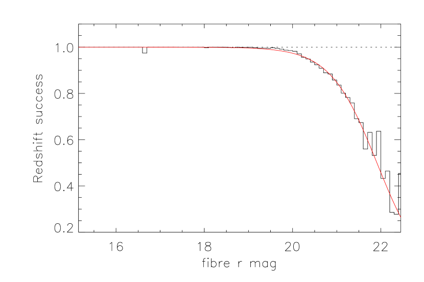
as a function of , and is shown in Fig. 3.
Note that some spectra observed in poor conditions have been re-observed
at a later date in order to obtain this high success rate.
We see that redshift success rate is essentially 100 per cent for , declines gently to around 98 per cent by and then declines steeply at fainter magnitudes. We have fitted a sigmoid function to the binned success rate. Sigmoid functions have previously been used to model survey completeness, e.g. by Ellis & Bland-Hawthorn (2007). Our best-fit sigmoid function has parameters mag-1, mag, shown by the red line in Fig. 3, and we use this fit in determining redshift success rate.
2.3.4 Galaxy weights
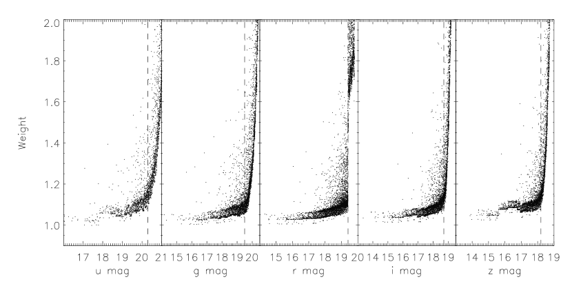
Each galaxy is given a weight which is equal to the reciprocal of the product of the imaging completeness, target completeness and redshift success rate. Imaging completeness is determined from the galaxy’s apparent -band half-light surface brightness, by linear interpolation of the curve in Fig.1. Target completeness is determined separately in each band from the galaxy’s magnitude according to Fig. 2 and the spectroscopic success rate is determined from the sigmoid function fit described in section 2.3.3.
The weight assigned to galaxy is then
| (2) |
These weights, as a function of magnitude in each band, are shown for a randomly selected 5 per cent of galaxies in Fig. 4. The majority of galaxies brighter than our magnitude limits have weight , with a small fraction extending to .
2.4 Velocity corrections
The redshifting software runz (Saunders, Cannon & Sutherland, 2004) provides heliocentric redshifts. Before converting heliocentric redshifts to any other velocity reference frame, we first eliminate likely stars from our sample by rejecting objects with a heliocentric redshift ( km/s). This lower redshift cut is conservatively chosen, as the 2nd Catalogue of Radial Velocities with Astrometric Data (Kharchenko et al., 2007) includes only one star with radial velocity km/s, and the vast majority of Galactic stars have km/s. Furthermore, Fig. 7 of Driver et al. (2011) shows that the redshift-error distribution for GAMA is essentially zero by km/s.
Having eliminated 2111 likely stars from our sample, heliocentric redshifts are converted to the CMB rest frame according to the dipole of Lineweaver et al. (1996). For nearby galaxies (), we apply the multiattractor flow model of Tonry et al. (2000). Note there are triple-valued solutions of over a small range in G12 (near the Virgo cluster), here the average distance is used. The solution is tapered to from to (see Baldry et al. 2011 for details). We will see later that the Tonry et al. flow correction affects only the very faintest end of the LF.
2.5 -corrections
When estimating intrinsic galaxy luminosities, it is necessary to correct for the fact that a fixed observed passband corresponds to a different range of wavelengths in the rest frames of galaxies at different redshifts, the so-called -correction (Humason, Mayall & Sandage, 1956). The -correction depends on the passband used, the redshift of the galaxy and its spectral energy distribution (SED). Here we use kcorrect v4_2 (Blanton et al., 2003a; Blanton & Roweis, 2007) in order to estimate and apply these corrections. Briefly, this code estimates an SED for each galaxy by finding the non-negative, linear combination of five template spectra that gives the best fit to the five SDSS model magnitudes of that galaxy. kcorrect can then calculate the -correction in any given passband at any redshift. Before calling kcorrect itself, we use k_sdssfix to convert SDSS asinh magnitudes to the AB system and to add in quadrature to the random mag errors given in the SDSS database typical systematic errors of (0.05, 0.02, 0.02, 0.02, 0.03) mag respectively.
We determine -corrections in a passband blueshifted by . These magnitudes are indicated with a superscript prefix of 0.1, e.g. . This choice of rest frame allows direct comparison with most previously published LFs based on SDSS data.
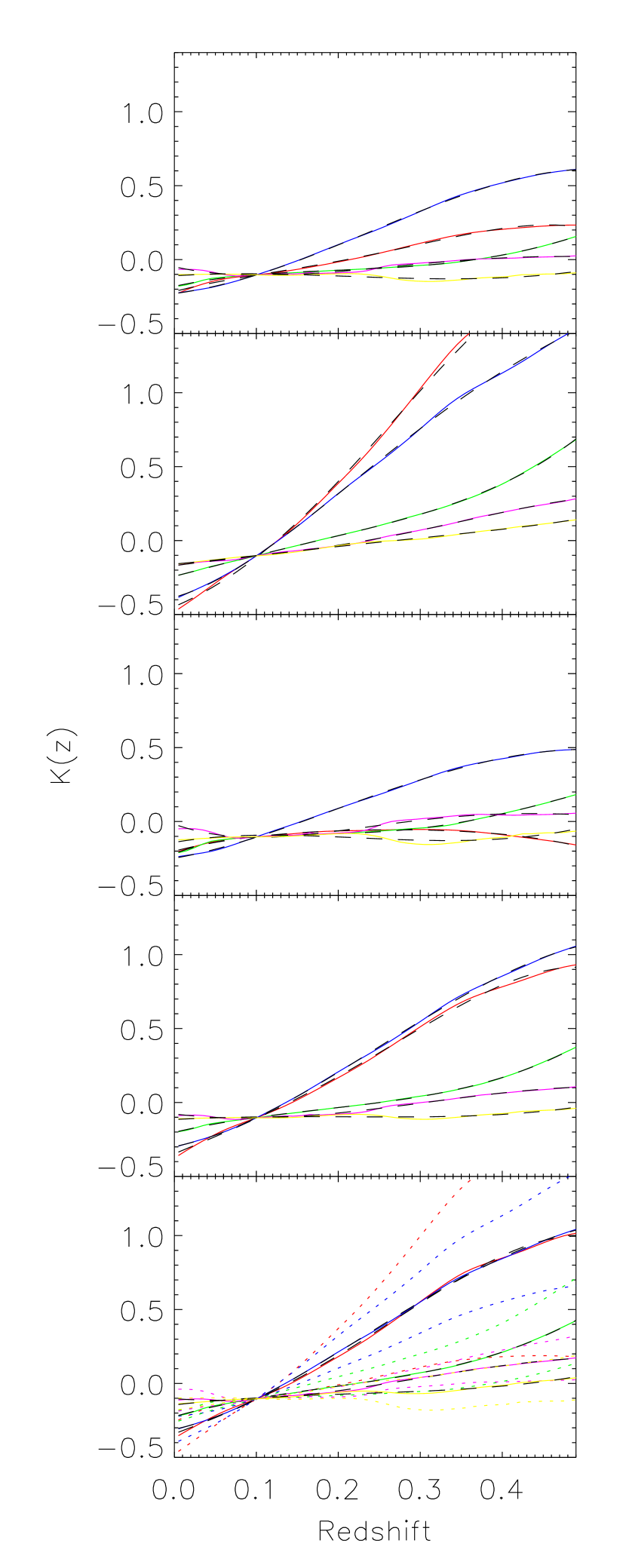
Our LF estimators require -corrections to be calculated for each galaxy at many different redshifts in order to work out visibility limits. To make this calculation more efficient, we fit a fourth-order polynomial , with , to the distribution for each galaxy and use this polynomial fit to determine -corrections as a function of redshift. Using a polynomial of this order, the rms difference between the kcorrect prediction and the polynomial fit is 0.01 mag or less in all five bands. Calculated -corrections and their polynomial fits are shown for the first four galaxies in our sample, along with the median -corrections and the 5 and 95 percentile ranges for the full sample, in Fig. 5.
Strictly, one should use heliocentric redshift when calculating -corrections, since they depend on the observed passband. However, for consistency with finding the minimum and maximum redshifts at which a galaxy would still be visible when using the LF estimator, we use the flow-corrected redshift as described in section 2.4. The difference in -correction when using heliocentric or flow-corrected redshift is entirely negligible.
2.6 Colour sub-samples
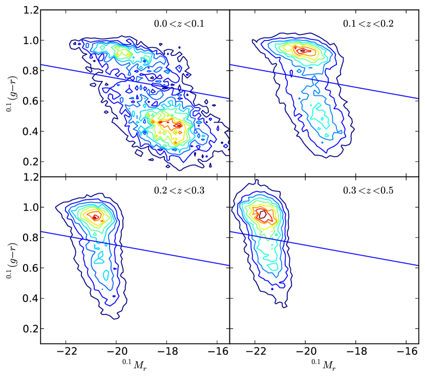
As well as analysing flux-limited samples of galaxies in the bands (hereafter the combined sample), we separate the galaxies into blue and red sub-samples. Following Zehavi et al. (2011), we use a colour cut based on -corrected model colour and absolute -band magnitude that is insensitive to redshift:
| (3) |
We have adjusted the zero-point of 0.21 mag in Zehavi et al. (2011) to 0.15 mag in order to better follow the ‘green valley’ and to get more equal-sized samples of blue and red galaxies. This colour cut works well at all redshifts (Fig. 6), although we see that the colour bimodality becomes far less obvious beyond redshift due to the lack of low-luminosity, blue galaxies at these high redshifts.
Although colour bimodality is more pronounced in colour, e.g. Strateva et al. (2001), Baldry et al. (2004), -band photometry, even after forming a ‘pseudo-Petrosian’ magnitude (equation 1) is rather noisy, and so we prefer to base our colour cuts on the more robust colour. This colour cut (in the original form of Zehavi et al.) has also been used to investigate the angular clustering of galaxies by Christodoulou et al. (2011). One should also note that colour is not a proxy for galaxy morphology: many red galaxies are in fact dust-obscured disc galaxies (Driver et al. in prep.).
2.7 Outlier inspection
| post_class | mag | mag |
|---|---|---|
| 1 OK | 4,743 | 299 |
| 2 QSO | 18 | 0 |
| 3 Major shred | 68 | 62 |
| 4 Minor shred | 0 | 7 |
| 5 Problem deblend | 151 | 16 |
| 6 Bad sky background | 246 | 14 |
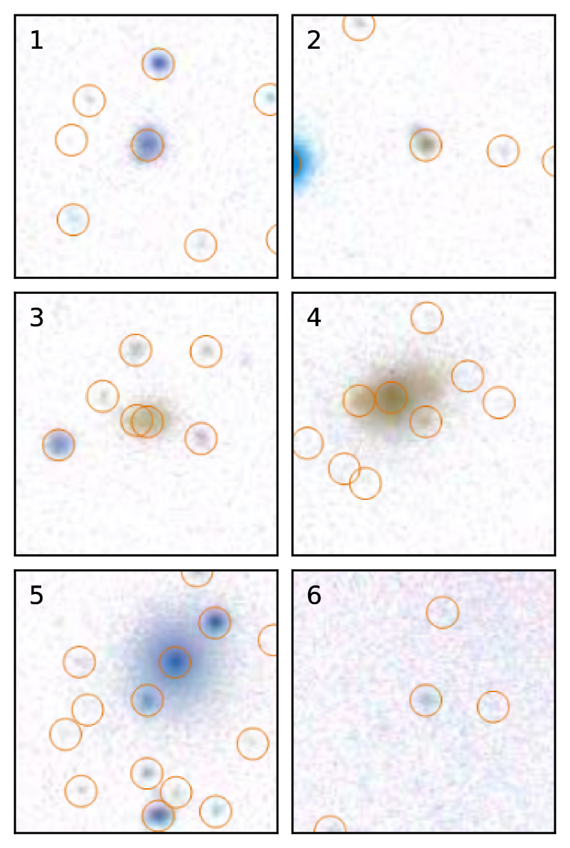
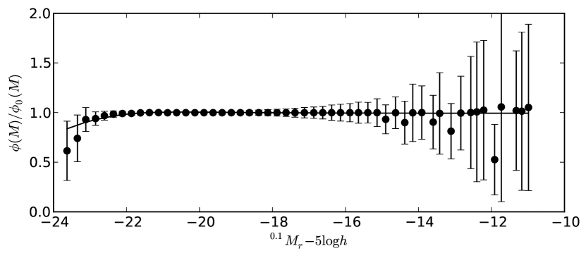
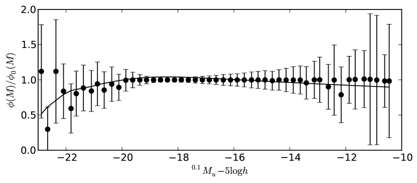
We measure the LF over a very wide range of luminosities, to mag in the band. Galaxies at the extremes of this luminosity range are very rare in a flux-limited survey, due either to their intrinsic low number density at high luminosity or small detection volume at low luminosity, and thus it is likely that a significant fraction of these putative extreme objects are in fact artifacts due to incorrectly assigned redshifts or magnitudes. The first author has therefore inspected image cutouts showing SDSS image detections of 5,226 very luminous GAMA targets with mag and 398 very faint targets with mag. We choose the band to select luminous outliers since the -band LF shows the largest bright-end excess.
Table 1 shows how the inspected images were classified. The classification codes, which we call post_class in order to distinguish them from the pre-target-selection vis_class have the following meanings.
-
(1).
OK — nothing from the image would lead one to expect poor photometry for that object.
-
(2).
The object looks like a QSO, i.e. blue and point-like. This classification is ignored in the analysis (treated as OK) due to the difficulty of distinguishing QSOs and compact blue galaxies from the imaging data alone.
-
(3).
The central part of a galaxy which has been shredded into multiple detections. It is likely that the luminosity is somewhat underestimated in these cases.
-
(4).
The target is a minor part of a shredded galaxy. Luminosity is likely to be greatly underestimated.
-
(5).
The galaxy is very close to a second object which either has not been deblended, or is likely to significantly affect the estimated luminosity in either direction.
-
(6).
Photometry is likely severely compromised by rapidly varying sky background due typically to the presence of a nearby saturated star.
Examples of objects with these classifications are shown in Fig. 7. In practice, there is some ambiguity in assigning a galaxy with classification 4 or 5, but as far as the LF analysis is concerned, it makes no difference.
These inspections were based on version 10 of the GAMA tiling catalogue, excluding objects with vis_class = 2–4. The major and minor shreds in Table 1 have also been inspected by IKB. In the case of major shreds, we have summed the flux from the components of the shredded galaxy to derive a ‘deblend-fixed’ magnitude. In total, 281 GAMA-I galaxies have had their magnitudes fixed in this manner.
In the case of six minor shreds which both JL and IKB agreed on, the value of vis_class has been set equal to 3 in the latest version (v16) of the tiling catalogue.
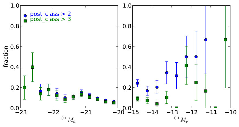
The fractions of galaxies with post_class of 3 or 4 or higher as a function of and are shown in Fig. 8. We see in the left panel that by magnitudes of , less than 10 per cent of objects have suspect photometry. Once we allow for fixing of over-deblended galaxies, a similar fraction of objects with have suspect photometry (right panel).
For our analysis, we have chosen to exclude any galaxies with post_class of 4 or higher, i.e. we include major shreds with fixed fluxes but exclude minor shreds, problem deblends and bad sky objects. Fig. 9 shows the ratio of the and band LFs using post_class galaxies to that determined using all galaxies. We see that excluding objects with suspect photometry has a relatively minor effect on the determined LF: the very bright end and some faint-end bins are systematically lower by up to 50 per cent; these changes are comparable to the size of the error bars.
Finally, we note that Brough et al. (2011) have independently checked a sample of GAMA galaxies with the lowest detected H luminosity. Our four faintest -band luminosity galaxies are also in the Brough et al. sample.
3 Estimating the luminosity function and its evolution
3.1 Parameterizing the evolution
In order to parametrize the evolution of the galaxy LF, we follow Lin et al. (1999) in assuming a Schechter (1976) function in which the characteristic magnitude and galaxy density are allowed to vary with redshift, but where the faint-end slope is assumed to be non-evolving.444Evolution in the LF faint-end slope with redshift is still rather poorly constrained. Ellis et al. (1996) claim that steepens with redshift, due to an increase in the number of faint, star-forming galaxies at . Ilbert et al. (2005) also measure a possible steepening of with redshift. In contrast, Liu et al. (2008) find that gets shallower at higher redshifts. Our assumption of fixed is largely based on practical necessity, since can only be reliably measured at redshifts from the GAMA data.
Specifically, in magnitudes, the Schechter function is given by
| (4) |
where the Schechter parameters , and vary with redshift as:
| (5) | ||||
Here the fiducial redshift is the same redshift to which magnitudes are -corrected, in our case . The Schechter parameters , and and evolution parameters and are determined via the maximum-likelihood methods described by Lin et al. (1999).
First, the shape parameters , and luminosity evolution parameter are fit simultaneously and independently of the other parameters by maximising the log likelihood
| (6) |
Here, is the incompleteness correction weighting (equation 2) and the probability of galaxy having absolute magnitude given its redshift is
| (7) |
where , are the absolute magnitude limits of the sample, , are the minimum and maximum absolute magnitudes visible at redshift , and is the differential LF given by (4).
The density evolution parameter and normalization cancel in the ratio in (7) and so must be determined separately. Lin et al. show that the parameter may be determined by maximising the second likelihood
| (8) |
where
| (9) |
where , are the redshift limits of the sample, , are the redshift limits over which galaxy may be observed, given the survey’s apparent magnitude limits and its absolute magnitude evolution-corrected to redshift zero, . Note that the value of is independent of the fiducial redshift .
Finally, we fit for the overall normalisation . We depart slightly from the prescription of Lin et al. (1999) here. In place of their equation 14, we use a minimum variance estimate of the space density of galaxies:
| (10) |
where is the galaxy selection function, a redshift weighting function chosen to give minimum variance and is the volume element at redshift . The selection function for galaxies with luminosities to is
| (11) |
Note that the integration limits in the numerator depend on the assumed -correction. In this case, we use the median -correction of the galaxies in the sample under consideration: see Fig.5 for median -corrections for the full sample as a function of redshift. Our results change by much less than the estimated 1-sigma errors (see Section 3.5) if we use mean instead of median -corrections.
We adopt the redshift weighting function
| (12) |
where is the two point galaxy correlation function and is the mean incompleteness weighting. Provided converges on a scale much smaller than the depth of the survey, then this redshift weighting scheme (equation 12) minimizes the variance in the estimate of (Davis & Huchra, 1982). Larger values of weight galaxies at high redshift more highly; we assume . This value comes from integrating the flux-limited two-point galaxy correlation function of Zehavi et al. (2005), , to ; at larger separations the value of becomes uncertain. However, the results are not too sensitive to the value of , the estimated densities changing by less than 8 per cent if is halved. This possible systematic error is generally comparable to or less than the statistical uncertainty in (5– 25 per cent).
3.2 Luminosity density
Given our assumed evolutionary model, the predicted LD is given by
| (14) |
(Lin et al. 1999 equation 11), where
| (15) |
and is the standard Gamma function. In making this prediction, we are integrating over all possible luminosities, and hence extrapolating our Schechter function fits. This extrapolation introduces no more than 1 per cent in additional LD beyond that contained within our luminosity limits. We obtain luminosities in solar units using the following absolute magnitudes for the Sun in SDSS bandpasses: mag (Blanton et al., 2003b).
We also directly determine LD as a function of redshift by summing the weighted luminosities of galaxies in a series of redshift bins:
| (16) |
(Lin et al. equation 16). Here is the volume of redshift bin , the sum is over each galaxy in bin and the factor
| (17) |
(Lin et al. equation 17) extrapolates for the luminosity of galaxies lying outside the accessible survey flux limits.
3.3 Binned LF estimates
In order to assess how well the model (equation 5) parametrizes LF evolution, we also make non-parametric, binned, estimates of the LF in independent redshift ranges using the (Schmidt, 1968; Eales, 1993) and stepwise maximum likelihood (SWML, Efstathiou, Ellis & Peterson 1988) methods. We use 60 magnitude bins from to with and a series of redshift slices.

When estimating the LF over restricted redshift ranges, one has to be careful to only include magnitude bins that are fully sampled, since otherwise the LF will be underestimated in incompletely sampled bins, see Fig. 10. We therefore set the following magnitude limits for each redshift slice so that only complete bins are included:
| (18) |
Here, and are the flux limits of the survey, is the distance modulus, is the -correction for a galaxy with the median SED of those in the survey, and are the limits of the redshift slice under consideration, and and are the absolute magnitude limits of each bin. A bin should only be included if it satisfies both equations (18).
Again following Lin et al. (1999), we incorporate the galaxy incompleteness weights into the SWML maximum likelihood estimator by multiplying each galaxy’s log-probability by its weight before summing to form a log-likelihood (equation 6). In the estimate, we form a sum of the weight of each galaxy divided by the volume within which it is observable. We normalize the SWML estimates in each redshift slice to the estimates by imposing the constraint
| (19) |
where is the volume (within the redshift limits of each slice) over which a galaxy of absolute magnitude , being the mean galaxy absolute magnitude in bin , is visible. The predicted number of galaxies
| (20) |
may also be compared with the observed number of galaxies within each redshift range.
We can use our SWML LF estimates to assess the quality of the parametric fits using a likelihood ratio test (Efstathiou, Ellis & Peterson, 1988). In this test, we compare the log-likelihoods and given by equation (6) for the SWML and parametric estimates respectively. The log likelihood ratio is expected to follow a distribution with degrees of freedom. Here is the number of bins in the stepwise estimate and we subtract 1 degree of freedom for each of the fitted shape parameters , and and for the arbitrary normalisation.
To allow for the finite bin sizes and redshift ranges of the SWML estimates, we calculate binned estimates of the parametric fits. These are given by (Lin et al., 1999)
| (21) |
Here, the parametric LF is weighted by the number of galaxies at each magnitude and redshift, given by the factor . These binned versions of the parametric fits are also used when plotting the LFs. For absolute magnitudes in all plots, we use the weighted mean magnitude of the galaxies in each bin, rather than using the magnitude of the bin centre. This helps to overcome the bias due to the finite width of magnitude bins.
3.4 LF faint end
It is now widely recognised that a Schechter function provides a poor fit to galaxy LFs when measured over a wide range of magnitudes (e.g. Blanton et al. 2005b). In order to parametrize the faint end, we separately analyse a low redshift () subset of the data and fit (non-evolving) double power-law Schechter functions.
We use the parameterization of Loveday (1997), namely
| (22) |
In this formulation, the standard Schechter function is multiplied by the factor , where is a transition luminosity between two power-laws of slope () and (). It is fitted to unbinned data using an extension to the method of Sandage, Tammann & Yahil (1979). With this four-parameter fit (the normalisation is fitted separately), one has to be careful to choose sensible starting values in order for the downhill simplex algorithm (scipy.optimize.fmin) not to get stuck in local minima of . (We also found that it helped to call the minimizer several times, using ‘best-fitting’ parameters from one function call as starting parameters for the next; was found to converge with 2–4 calls of the minimizer.)
Note that the double power-law Schechter function may equivalently be written as the sum of two Schechter functions, e.g. Blanton et al. (2005b); Baldry, Glazebrook, Driver (2008), a fact which comes in useful when integrating the LF.
When fitting a double power-law Schechter function, the likelihood ratio test has degrees of freedom (cf. section 3.3).
3.5 Error estimates
Schechter and evolution parameter estimates are strongly correlated, and so in Section 4 we present 95 per cent likelihood contour plots of shape parameters , , , and evolution parameters , . For uncertainties in tabulated measurements, we estimate errors using the jackknife technique, as follows. We divide the GAMA survey area into nine regions, each deg 2. We then calculate the LF and LD using the methods discussed above, omitting each region in turn. For any parameter , we may then determine its variance using
| (23) |
where is the number of jackknife regions and is the mean of the parameters measured while excluding region . The jackknife method has the advantage of providing error estimates which include both uncertainties in the fitted parameters as well as sample variance.
The sample variance in galaxy density may also be determined using:
| (24) |
(Davis & Huchra, 1982; Efstathiou, Ellis & Peterson, 1988), where is defined in (12) and is the volume of each sample between redshift limits.
For errors on binned LFs, we use Poisson errors for estimates and an inversion of the information matrix for SWML estimates (Efstathiou, Ellis & Peterson, 1988).
4 Results
Before presenting our main results, we first check the effects of correcting for imaging completeness and the choice of flow model in converting redshifts to distances.
4.1 Imaging completeness correction
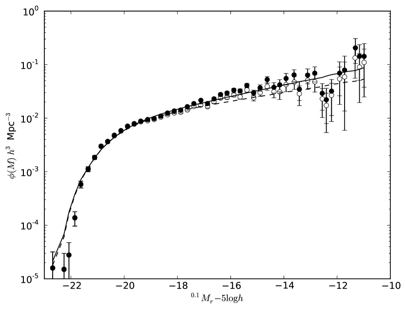
In Fig. 11, we compare -band LFs calculated for the combined sample, with distances calculated using the Tonry et al. (2000) multiattractor flow model, with and without the correction for imaging completeness described in Section 2.3.1. As expected, we see that applying imaging completeness corrections boosts the LF faint end, while barely changing the bright end. The changes in fitted Schechter parameters due to imaging completeness corrections are tabulated in Table 2. Future plots and tabulated parameters will include imaging completeness corrections; approximate uncorrected Schechter parameters may be obtained by subtracting the appropriate quantities listed in Table 2.
4.2 Effects of velocity flow model
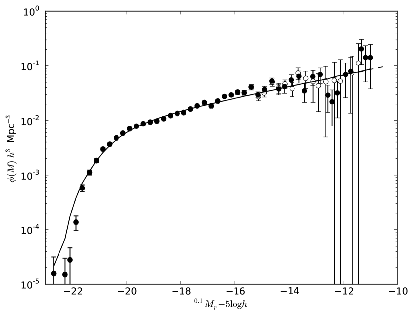
Luminosities of galaxies at the extreme faint end of the LF, being very close by, will be sensitive to peculiar velocities. In Fig. 12, we compare -band LFs calculated using the CMB reference frame (Lineweaver et al., 1996) and the Tonry et al. (2000) multiattractor flow model for galaxies at low redshift (). We see that the CMB-frame and flow model LFs only begin to differ at the extreme faint end, mag, and even at these faint magnitudes the differences are not large given the size of the error bars. In particular, the recovered Schechter parameters are indistinguishable between the two velocity frames. Subsequent analysis will use the Tonry et al. flow model to determine luminosities.
4.3 Luminosity function faint end
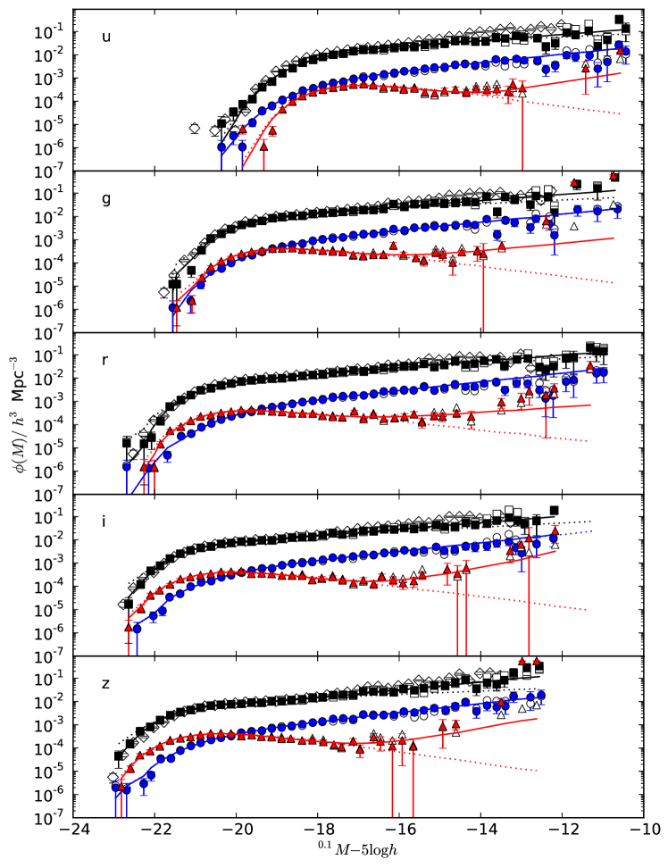
Having looked at the effects of incompleteness and flow corrections, we now study in detail the faint end of the LF for low redshift () galaxies. Fig. 13 shows the LFs for our three (combined, blue and red) samples in the bands. Also shown are LFs corrected for surface brightness incompleteness by Blanton et al. (2005b) from the New York University Value-Added Galaxy Catalog (NYU-VAGC) low-redshift sample (Blanton et al., 2005a). Since these Blanton et al. LFs were calculated using restframe -corrections, we apply an offset of to their absolute magnitudes in order to convert to our band-shifted -corrections. Our faint-end LFs are systematically lower than those of Blanton et al., particularly in the band. The difference can largely be explained by the different flow models used by Blanton et al. and in the present analysis. Re-analysing the Blanton et al. data using the Tonry et al. flow model results in much better agreement (Baldry et al., 2011) — the extra 1.7 mag depth of the GAMA versus the SDSS main galaxy sample means that uncertainties due to the flow model affect the measured LF only at a correspondingly fainter magnitude.
Table 3 shows the number of galaxies and absolute magnitude limits for each sample, along with the parameters of standard Schechter function fits and luminosity densities. Only for blue galaxies in the , and bands does a standard Schechter function provide a statistically acceptable fit to the data at the 2 per cent level or better. For red galaxies, we observe a decline in number density faintwards of the characteristic magnitude with a subsequent increase in faint-end slope at . For the red galaxies, and the combined sample, a double-power-law Schechter function (22) is required to fit the shape of the observed LFs. These findings are in apparent agreement with the predictions of halo occupation distribution models, e.g. Brown et al. (2008), in which luminous red galaxies are central galaxies, but fainter red galaxies are increasingly more likely to be satellites in relatively massive halos. An alternative perspective is provided by Peng et al. (2010), who explain the change in faint-end slope of red galaxies via a simple picture for the quenching of star formation by the distinct processes of ‘mass quenching’ and ‘environment quenching’. Our results provide the most precise demonstration of the changing faint-end slope of red galaxies to date.
However, the observed upturn needs to be interpreted with caution, since, from a quick visual inspection, the 164 faint ( mag), red galaxies that comprise the upturn include a significant fraction ( per cent) of galaxies that appear to be disc like, as well as a number of artifacts. It thus seems likely that dust-reddened disc systems, as well as dwarf galaxies with intrinsically red stellar populations, contribute to the faint-end upturn in the red galaxy LF. Future work will investigate the LF dependence on morphology and dust reddening, utilising GAMA’s multi-wavelength coverage.
Double-power-law Schechter function fits are given in Table 4. Likelihood ratio tests show that the double-power-law Schechter function provides significantly better fits than the standard Schechter function for the combined and red galaxy samples, at least for the redder bands. For the blue galaxies, however, the double-power-law Schechter function fits are actually worse than the standard Schechter function fits when taking into account the two additional degrees of freedom.
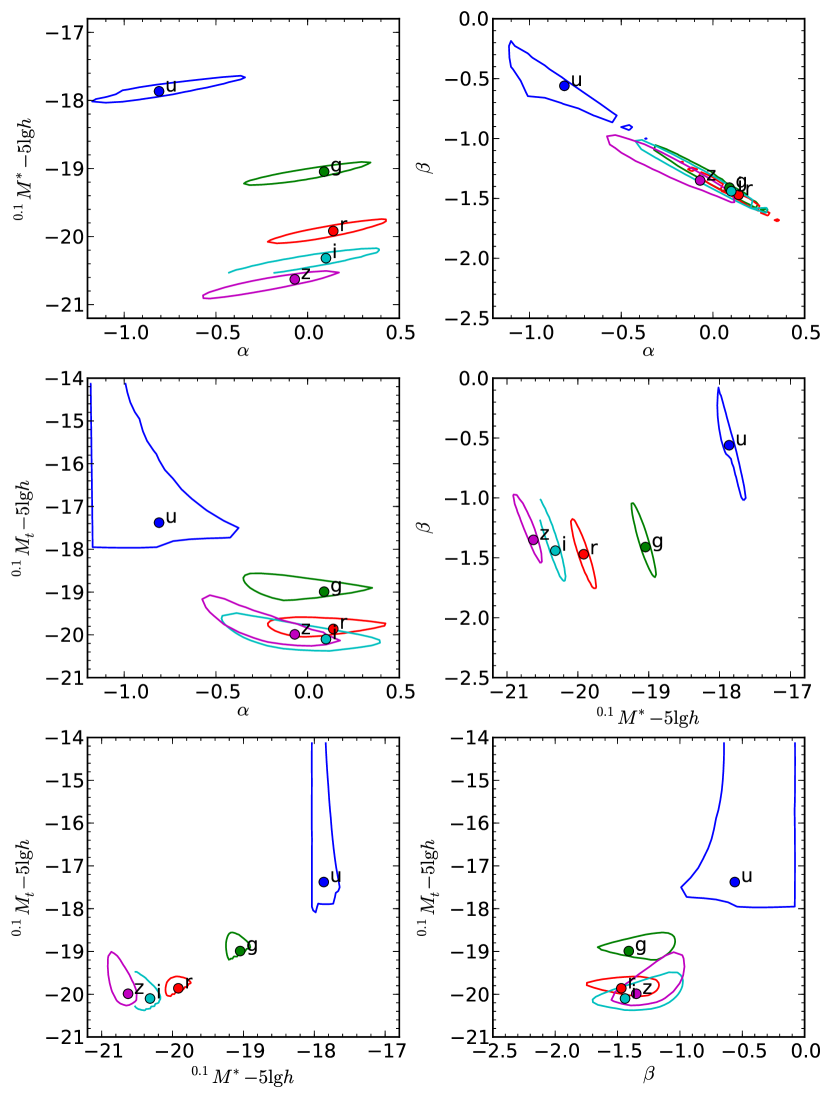
The quoted errors need to be treated with caution due to strong correlations between the parameters, particularly in the case of the five-parameter, double power-law Schechter function fits. Fig. 14 shows likelihood contours for each pair of parameters from and for the combined sample. We see that and individually are very poorly constrained, with an uncertainty . However, the overall faint-end slope is very well constrained, with a consistent value in all five passbands for the combined sample. For blue galaxies, and for red galaxies, . Consistent faint-end slopes are found for the stellar mass function (Baldry et al., 2011) . Also from Fig. 14, we see that the characteristic magnitude is positively correlated with slope but negatively correlated with . The transition magnitude is only weakly correlated with either slope parameter or and almost completely uncorrelated with the characteristic magnitude .
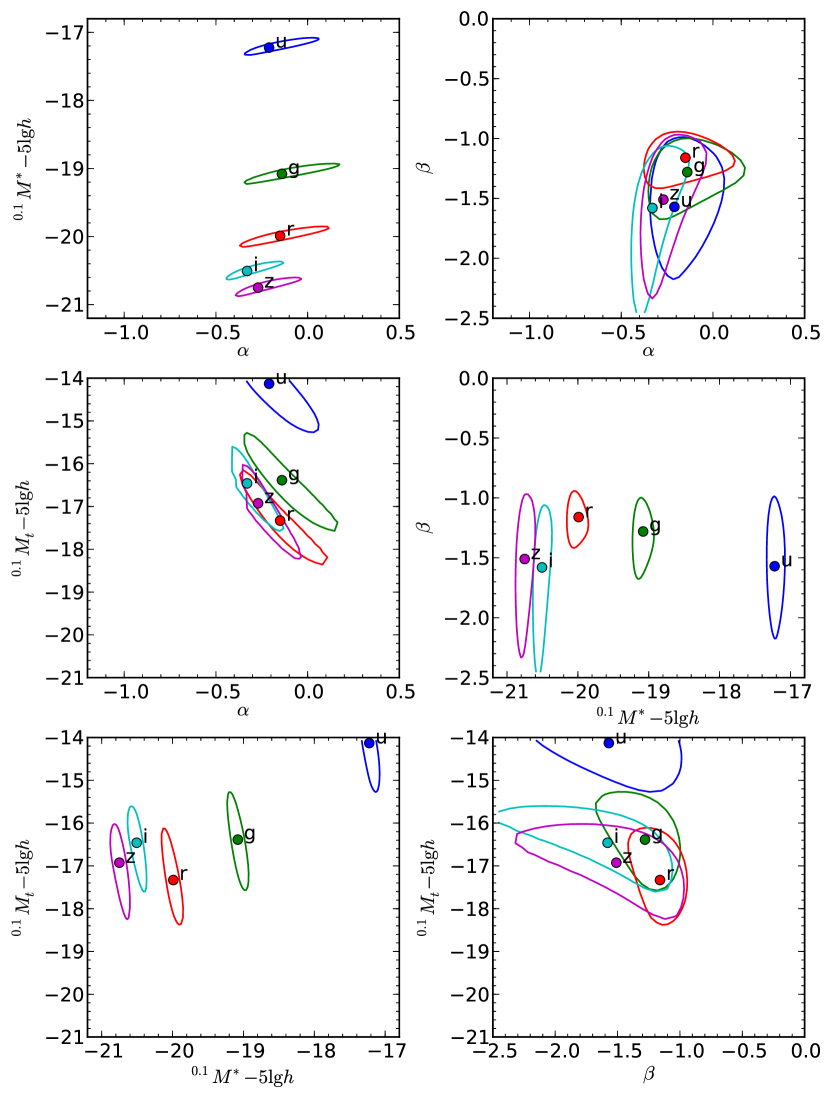
Fig. 15 shows likelihood contours for the red sample. We see that, while still uncertain, the slope parameters and are only weakly correlated. The characteristic magnitude is positively correlated with but almost completely uncorrelated with . The transition magnitude is strongly anti-correlated with and virtually independent of .
Since the shape of the blue galaxy LF is reasonably well fitted by a standard Schechter function, there are huge degeneracies between the double power-law Schechter function parameters, and so the contour plots contain no useful information, and hence are not shown.
In summary, in analysing the faint end of the LFs, we have found that:
-
1.
While a standard Schechter function provides an acceptable fit to the blue galaxy LF in all bands, the red galaxy LF exhibits a decline just faintwards of followed by a pronounced upturn at magnitude . Such an LF is well-fitted by a double-power-law Schechter function.
-
2.
We caution that the faint end of the red galaxy LF is possibly dominated by dust-reddened systems, rather than by galaxies with intrinsically red stellar populations.
-
3.
Neither standard nor double-power-law Schechter function faint-end slopes show any systematic dependence on passband: while strongly colour-dependent, faint-end slopes are largely independent of passband.
-
4.
The characteristic magnitude (and to a lesser extent, the transition magnitude ) brightens systematically and significantly with passband effective wavelength.
4.4 Luminosity function evolution
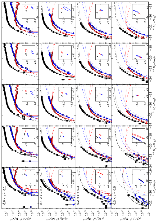
We present LFs for the combined, blue and red samples in the bands in four redshift ranges in Fig. 16. Table 5 gives the magnitude limits (chosen to exclude the upturn seen in the LF of red galaxies)555This choice of magnitude limits also corresponds closely to those of Blanton et al. (2003b)., observed and predicted numbers of galaxies, and Schechter and evolution parameters in each band. Qualitatively, the LFs appear to be well fitted by the parametric evolution model, although this model is formally excluded by the likelihood ratio test for almost every colour, band and redshift combination. Even by eye, we see that the evolving Schechter function fits are in extremely poor agreement with the and band non-parametric (SWML and ) estimates in the highest redshift range, in the sense that the model overpredicts the number density of luminous galaxies by almost an order of magnitude in the band. Equation 5 thus provides a poor fit to evolution of the - and -band LFs beyond and , respectively. It is very possible that the -band flux of more luminous, higher redshift galaxies is being dominated by AGN. We intend to investigate the LFs of AGN-dominated/starforming/quiescent galaxies in a future paper.
In addition to the parametric fit, we also fit Schechter functions to the SWML estimates for each redshift slice using least-squares. Because the LF faint end is poorly sampled at redshift , we only fit for all three Schechter parameters , and in the lowest-redshift slice. At higher redshifts we hold fixed and allow only and to vary. The results of these fits are shown as dashed lines in Fig. 16 and the insets show 95 per cent likelihood contours of (, ). These least-squares fits are for illustration only. In order to calculate the parameters and given in Table 5, and shown below in Fig. 19, we sub-divide into eight redshift bins, perform least-squares fits to the SWML estimates in each, and then fit straight lines to and versus redshift. We now discuss LF evolution separately, for the , and bands.
4.4.1 -band evolution
We observe a gradual brightening of for all samples between and , and already a bright-end excess above a Schechter function is becoming apparent. By , the evolving model provides a very poor fit to the non-parametric estimates: the former is much steeper than the latter, and by the parametric fit over-predicts the number density of galaxies by almost an order of magnitude. From the least-squares fits to the non-parametric estimates, we see a dramatic brightening of in the highest redshift range (there are too few red galaxies to obtain a sensible LF fit in this bin). This is due to the very shallow slope at the bright end of the LF, leading the Schechter fit to prefer brightening to increasing . In reality, we suspect that this shallow slope is caused by an increasing fraction of highly-luminous AGNs, rather than by such strong luminosity evolution in non-active galaxies. An alternative explanation is that photometric errors in the band are manifesting themselves as unrealistically strong luminosity evolution. This possibility will explored when VST KIDS data become available in the GAMA regions.
4.4.2 -band evolution
The parametric model provides a good fit out to redshift , beyond which a bright-end excess results in an over-prediction of the LF relative to the non-parametric estimates. From these latter estimates, one sees that the number density of blue galaxies is gradually increasing with redshift, whereas red galaxies show the opposite trend. Photometric errors are less likely to be a problem in the than in the band, and so again we suspect that AGNs are dominating the bright end of the LF at higher redshifts. This interpretation does not necessarily imply rapid evolution of the AGN population — the volume sampled at low redshifts is simply too small to detect them in significant numbers.
4.4.3 -band evolution
Evolution in the , and bands is qualitatively very similar, and so we discuss them together. The parametric model provides a reasonable fit in all redshift slices, although it should be said that the formal fit probabilities from the likelihood ratio test are mostly below 1 per cent. This does not necessarily mean that the model is a poor fit, as we see from simulations (Appendix A) that the non-parametric LF estimates are biased when the underlying LF is evolving. The likelihood ratio test provides improved probabilities when we consider narrower ranges in redshift. From the non-parametric fits, we see that brightens with redshift for all samples. At low redshifts, red galaxies have a much higher space density than blue, but as redshift increases, the density of red galaxies drops and that of blue galaxies increases, until blue galaxies come to dominate by redshifts .
4.4.4 Comparison with previous results
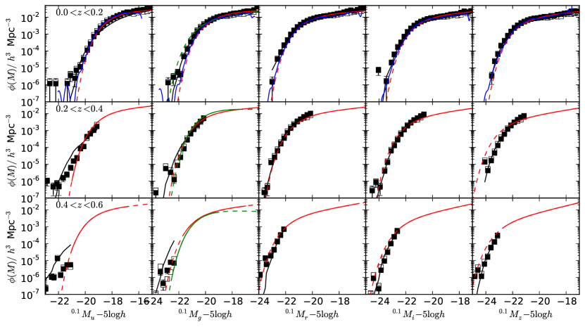
We compare our evolving LFs with previous estimates in Fig. 17. Here we plot the LFs in three redshift ranges (0.002, 0.2], (0.2, 0.4] and (0.4, 0.6]. We choose these ranges to coincide with the first three redshift bins used by Ilbert et al. (2005) in their analysis of the VIMOS-VLT deep survey (VVDS). Following these authors, we assume approximate correspondence between the restframe and the passbands, and assume that . Their LFs are shown as red lines: solid over the magnitude range actually fitted, dashed where extrapolated.
In the low-redshift range (top row), we also show the non-parametric LF estimates of SDSS galaxies from Blanton et al. (2003b) as blue lines. Their estimates are in good agreement with our non-parametric SWML and estimates except that we see a slightly higher density of luminous galaxies, particularly in the band ( mag). This difference is likely to be due to the greater depth of the GAMA sample compared with SDSS: the mean redshift in this range is for GAMA versus for SDSS. The GAMA sample thus contains a higher fraction of more distant and hence more evolved galaxies. The VVDS Schechter fits in the lowest redshift bin show a slightly lower density of luminous galaxies than seen in GAMA and SDSS. Note, however, that the bright end of the low-redshift LF is very poorly constrained by Ilbert et al. due to their bright apparent magnitude limit of . The zCOSMOS band LF from Fig. 1 of Zucca et al. (2009) (Zucca private communication, green line) shows a bright-end excess relative to GAMA and to VVDS. While reaching about 1.5 mag brighter than VVDS, the zCOSMOS low-redshift LF still relies on extrapolation at magnitudes brighter than mag.
At intermediate redshifts (middle row), our LFs are in good agreement with VVDS and zCOSMOS apart from an excess of -bright galaxies in GAMA, and, conversely, a much higher bright-end fit by VVDS in the () band. This latter discrepancy is almost certainly due to poor coverage of the bright end of the band LF at redshifts by VVDS.
In the highest redshift range (bottom row), the extrapolation of the VVDS Schechter fit shows a higher abundance of luminous galaxies in the redder bands than GAMA. In this redshift range the comparison is not quite fair, since GAMA contains very few galaxies beyond , and so much of the VVDS excess is likely to be due to galaxies in the redshift range .
4.4.5 Schechter parameter likelihood contours
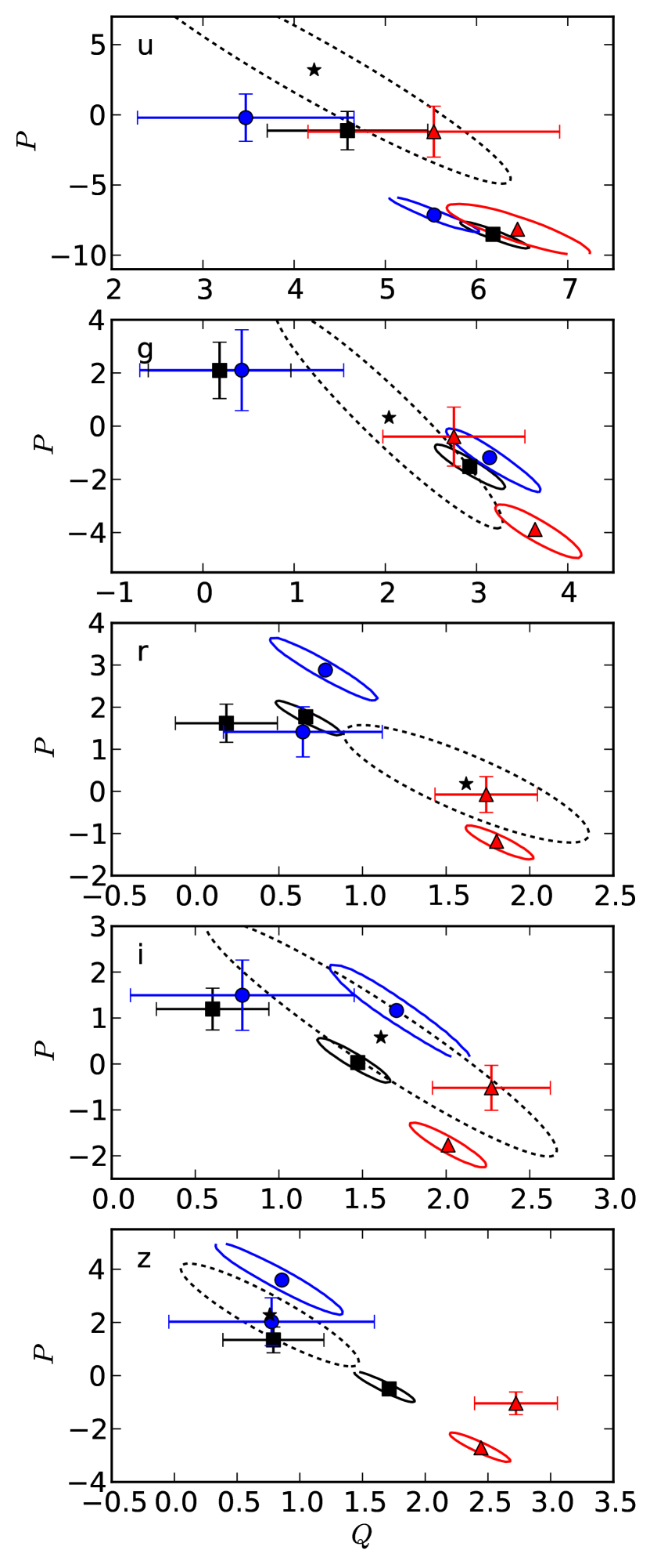
likelihood contours for the Schechter parameters (, ), determined using the parametric fits, are shown in Fig. 18. For the combined sample, we find roughly consistent faint-end slopes in all bands. The slightly steeper slope seen in the band is most likely due to the fact that GAMA is selected in the band, and hence we probe slightly further down the LF in this than the surrounding bands. Similarly, the slightly steeper slopes in our fits to the low-redshift sample (Table 3) are due to the inclusion of fainter-magnitude galaxies in those fits. As expected, increases systematically in brightness with increasing wavelength from to . Red galaxies have systematically shallower faint-end slopes ( in ) than blue galaxies () in all bands. The characteristic magnitudes are fainter for red galaxies than for blue in the bands and are comparable in the bands.
Fig. 18 also shows Schechter function parameters estimated from the SDSS main galaxy sample by Blanton et al. (2003b). We find systematically steeper faint-end slopes (apart from in the band) and brighter characteristic magnitudes (apart from the band). Since our non-parametric estimates are in good agreement (Fig. 17), these differences most likely arise due to strong degeneracies between the parameters , and : (, ), (, ) and (, ) are all positively correlated.
4.4.6 Evolution parameter likelihood contours
In Fig. 19 we show likelihood contours for the luminosity evolution parameters and from our parametric fits, along with estimates of these quantities and their errors from least-squares fits of Schechter functions to the SWML estimates made in eight redshift ranges. The differences between the estimates of these parameters are frequently larger than the formal errors associated with each method. This indicates that our assumption of linear evolution of and with redshift is only approximate.
For the combined sample, luminosity evolution is least in the band (), increasing to in the and bands. Luminosity evolution is even more pronounced in the and bands ( and 6.2, respectively), although, as previously noted, the parametric model performs very poorly in these bands, and so these values are unreliable at best. Luminosity evolution is more pronounced for the red galaxy population than the blue.
Blue galaxies exhibit positive density evolution, ( in all bands apart from and , in all bands apart from ), whereas red galaxies show negative density evolution, both and are negative in all bands. This observation is in good qualitative agreement with an analysis of the zCOSMOS survey by Zucca et al. (2009), who find that both early- and late-spectroscopic-type galaxies brighten in by mag over the redshift range to , but that for early types decreases by a factor over the same redshift range; for late types increases by a factor .
Density evolution for the combined sample is positive in the band; in other bands is either negative or consistent with zero, compensating for the stronger luminosity evolution in these bands. Thus the contrary density evolution of blue and red galaxies largely cancels out in the combined sample. For all bands and samples, the evolution parameters (, ) are strongly anticorrelated. We remind the reader that the maximum-likelihood luminosity evolution is determined along with and , independently of the normalisation of the LF. Density evolution does depend on the fitted value of , as well as the Schechter parameters, resulting in the observed anti-correlation between and . In the redder bands, , the combined LD evolution is stronger for blue galaxies, , than for red, .
Fig. 19 also shows evolution parameters determined from the SDSS main galaxy sample by Blanton et al. (2003b). The likelihood contours intersect in , and narrowly miss in and . In the band we find weaker luminosity evolution and a compensating stronger density evolution, vice versa in . Our least-squares fits to the SWML estimates in the band yield comparable estimates to Blanton et al. (2003b). Their density evolution, unlike ours, is positive, but has a very large error.
Although sampling a smaller volume, the GAMA data analysed here have a mean redshift compared with for the data analysed by Blanton et al. We thus have a longer redshift baseline over which to measure evolution.
Hopkins (2004), in an analysis combining constraints from the star formation rate density of the Universe and 1.4-GHz radio source counts, found , for the star forming galaxy population666Note that Hopkins actually models evolution as and .. This measurement, sensitive to the star-forming population up to , is consistent with our parametric fit results for blue galaxies in the band at the low-redshift end of this range. However, given the very large discrepancy between and for blue galaxies in the band, the apparent agreement may be fortuitous.
For red galaxies, Brown et al. (2007) find that in the band brightens by mag from redshift to while declines by about 25 per cent, in qualitative agreement with our results
4.4.7 Evolution summary
To summarize our findings regarding evolution of the LF:
-
1.
The evolutionary model (equation 5) provides a reasonable fit in the redder bands, , but performs poorly in the and bands, overpredicting the LF of luminous galaxies at high redshift. This is possibly due to a significant contribution from AGNs.
-
2.
Our non-parametric LF estimates are in good agreement with SDSS measurements at low redshift and with results from the VVDS and zCOSMOS surveys at higher redshifts, over magnitude ranges where our LF estimates overlap.
-
3.
There is a strong degeneracy between the luminosity and density evolution parameters and . One should be wary in using them in isolation, e.g. using the parameter to apply evolutionary corrections.
-
4.
Nevertheless, red galaxies in all bands show evidence for positive luminosity evolution () and negative density evolution ().
-
5.
Blue galaxies show less luminosity evolution but show evidence for positive density evolution.
-
6.
The observation of decreasing number density of blue galaxies but increasing number density of red galaxies with cosmic time implies that the transition from blue cloud to red sequence is an important and ongoing phenomenon since redshifts .
-
7.
The combined luminosity plus density evolution is stronger for blue than for red galaxies.
4.5 Luminosity density evolution
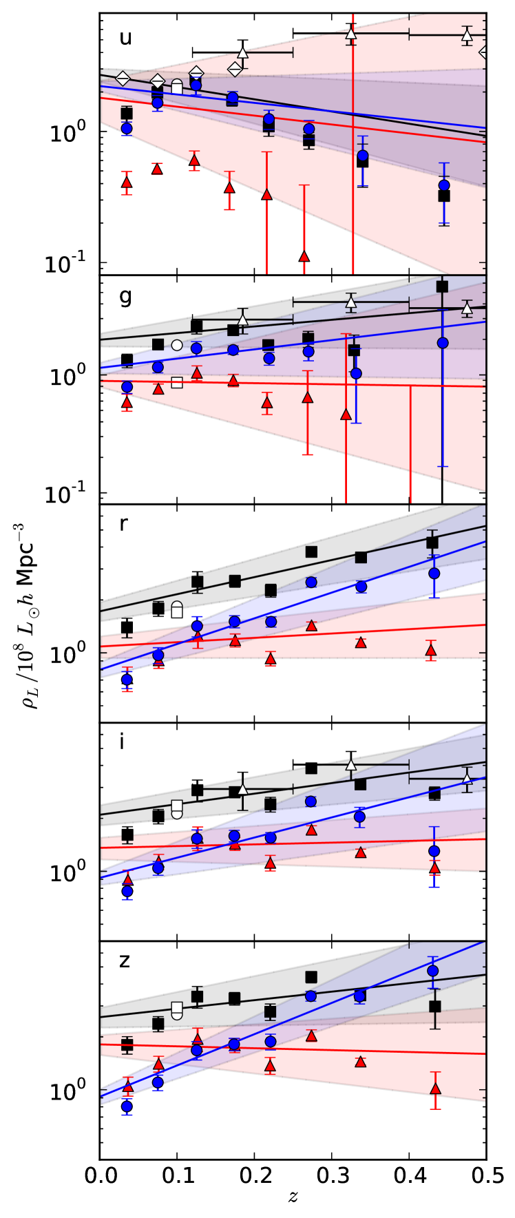
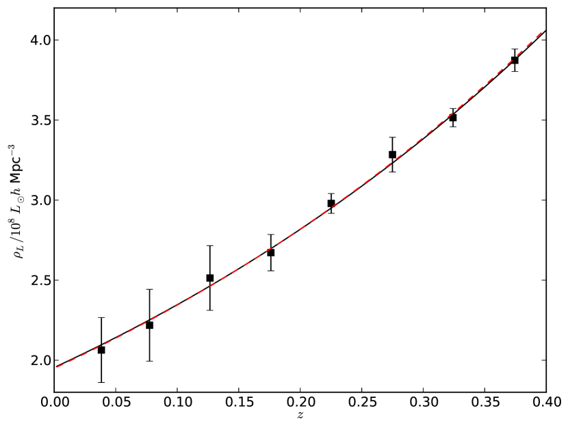
As we have seen in the previous section, while it can be difficult to isolate the effects of luminosity and density evolution, evolution in LD is better constrained. Fig. 20 shows the LD measured in eight redshift bins up to , according to equation 16, along with the prediction of the parametric model (equation 14). These results are tabulated in Table 6. For the combined sample, in all bands other than , we see LD increasing with redshift, steeply between redshifts and , slightly more gradually thereafter. The blue galaxy LD increases more steeply with redshift than the combined sample. The LD of red galaxies barely evolves with redshift beyond , thus the relative contribution to LD from blue galaxies comes to dominate by redshifts . Given our choice of colour cut (equation 3), red and blue galaxies contribute roughly equally to the LD in the and bands at low redshifts (), red galaxies are slightly dominant in the band but under-represented in and bands.
Fig. 20 also shows the LD estimated from the SDSS by Blanton et al. (2003b) and Montero-Dorta & Prada (2009) at a mean redshift of . Our results are in excellent agreement with those of Blanton et al. (2003b). Montero-Dorta & Prada (2009) appear to have significantly underestimated the -band LD, although their estimates in other bands are in agreement with ours and those of Blanton et al. (2003b). Open triangles show LD estimates from CNOC2. We have taken the ‘Total’ values from table 3 of Lin et al. 1999 in , and bands, corresponding roughly to , and respectively. We convert the CNOC2 luminosity densities from physical units of W Hz-1 Mpc-3 to AB magnitudes using and then convert into Solar luminosities using the assumed absolute magnitudes of the Sun quoted in Section 3.2. The - and -band LD estimates are in reasonable agreement with our -and -band estimates, while the CNOC2 -band LD is many times larger than our -band LD at redshifts . Open diamonds show -band LD estimates from Prescott, Baldry & James (2009).
Note that our -and -band LD estimates will be adversely affected by the poor fit of the parametric model for LF evolution. The selection function in the denominator of equation (16) will be overestimated at high redshifts in these bands, and hence the summed LD itself will be underestimated, leading to the decline in LD with redshift seen for the band in Fig. 20.
Previous studies of LD evolution (e.g. Lilly et al. 1996; Lin et al. 1999; Bell et al. 2004; Baldry et al. 2005; Willmer et al. 2006; Faber et al. 2007; Prescott, Baldry & James 2009) have found that for blue and non-colour-selected galaxies, increases monotonically with redshift, while for red galaxies, it is approximately constant, with a possible decline beyond redshift . We have presented the most detailed investigation to date of LD evolution since redshift , finding consistent results in the and bands with previous analyses which have focused primarily on evolution beyond redshifts .
5 Conclusions
We have presented the first measurements of the galaxy LFs from the GAMA survey, after correcting for imaging, target and spectroscopic incompleteness. At low redshift (), the shapes of the blue galaxy LFs are reasonably matched, albeit not in detail, by standard Schechter functions. LFs for red galaxies show a noticeable dip at intermediate magnitudes, requiring double power-law Schechter functions to obtain an adequate fit. One should be cautious in interpreting this as the upturn predicted by halo occupation distribution models (e.g. Brown et al., 2008) and the Peng et al. (2010) quenching model, since the faint end of our red galaxy LF contains a significant fraction of edge-on disc systems, which are likely to be dust-reddened. We find consistent faint-end slopes in all bands, for the combined sample.
In order to determine evolution of the LF, we employ the parametric model of Lin et al. (1999) in which characteristic magnitude and log density are allowed to vary linearly with redshift. We test the parametric model by comparing with estimates using the and SWML estimates. We find that the , and bands are qualitatively well fitted by this model, although the model provides poor likelihood fits compared with SWML. The model predicts an excessively high number density in the and bands at high redshift, most likely due to QSO/Seyfert contamination (Montero-Dorta & Prada, 2009). With this caveat in mind, we find positive (i.e. increasing with redshift) luminosity evolution in all bands and for all colour samples. Luminosity evolution is stronger for red than for blue galaxies, with blue galaxies brightening by –1.5 mag per unit redshift, red galaxies brightening by –2.5 mag per unit redshift.
Number density evolution for blue galaxies is positive in the redder bands in which it can be reliably measured, while red galaxies exhibit negative density evolution. This observation of decreasing number density of blue galaxies but increasing number density of red galaxies with cosmic time implies that the transition from blue cloud to red sequence is an important and ongoing phenomenon since redshifts . Investigation of the mechanism that causes this transition will be the subject of future work, but it appears unlikely that mergers play a dominant role at these moderate redshifts, given the low merger fraction ( per cent or less) observed at low redshift by e.g. Conselice et al. (2009) and Lotz et al. (2011).
Luminosity density increases from redshift zero until , beyond which redshift it increases more gradually for the combined sample. The LD of red galaxies is roughly constant beyond , whereas that for blue galaxies keeps on increasing, leading to blue galaxies dominating the LD at higher redshifts.
In this paper, we have not considered the effects of internal dust extinction on the LF, nor have we considered the effects of using total as opposed to Petrosian magnitudes (Graham et al., 2005; Hill et al., 2011). These extensions to the analysis will be considered in a future paper, along with a measurement of the galaxy LF for AGN-dominated, star-forming and quiescent galaxies which, it is hoped, will resolve the problems encountered while attempting to fit an evolutionary model in the and bands.
Acknowledgements
JL acknowledges support from the Science and Technology Facilities Council (grant numbers ST/F002858/1 and ST/I000976/1). PN acknowledges financial support from a Royal Society URF and an ERC StG grant (DEGAS-259586). We thank Elena Zucca for providing her Schechter function fits to the zCOSMOS band LF (Zucca et al., 2009, Fig. 1) and Alister Graham, Simon Lilly and the referee for useful comments.
GAMA is a joint European-Australasian project based around a spectroscopic campaign using the Anglo-Australian Telescope. The GAMA input catalogue is based on data taken from the Sloan Digital Sky Survey and the UKIRT Infrared Deep Sky Survey. Complementary imaging of the GAMA regions is being obtained by a number of independent survey programs including GALEX MIS, VST KIDS, VISTA VIKING, WISE, Herschel-ATLAS, GMRT and ASKAP providing UV to radio coverage. GAMA is funded by the STFC (UK), the ARC (Australia), the AAO, and the participating institutions. The GAMA website is: http://www.gama-survey.org/.
Funding for the SDSS and SDSS-II has been provided by the Alfred P. Sloan Foundation, the Participating Institutions, the National Science Foundation, the U.S. Department of Energy, the National Aeronautics and Space Administration, the Japanese Monbukagakusho, the Max Planck Society, and the Higher Education Funding Council for England. The SDSS Web Site is http://www.sdss.org/. The SDSS is managed by the Astrophysical Research Consortium for the Participating Institutions. The Participating Institutions are the American Museum of Natural History, Astrophysical Institute Potsdam, University of Basel, University of Cambridge, Case Western Reserve University, University of Chicago, Drexel University, Fermilab, the Institute for Advanced Study, the Japan Participation Group, Johns Hopkins University, the Joint Institute for Nuclear Astrophysics, the Kavli Institute for Particle Astrophysics and Cosmology, the Korean Scientist Group, the Chinese Academy of Sciences (LAMOST), Los Alamos National Laboratory, the Max-Planck-Institute for Astronomy (MPIA), the Max-Planck-Institute for Astrophysics (MPA), New Mexico State University, Ohio State University, University of Pittsburgh, University of Portsmouth, Princeton University, the United States Naval Observatory, and the University of Washington.
References
- Abazajian et al. (2003) Abazajian K et al., 2003, AJ, 126, 2081
- Abazajian et al. (2004) Abazajian K et al., 2004, AJ, 128, 502
- Abazajian et al. (2009) Abazajian K et al., 2009, ApJSupp, 182, 543
- Adelman-McCarthy et al. (2008) Adelman-McCarthy J.K. et al. 2008, ApJS, 175, 297
- Baldry et al. (2004) Baldry I.K., Glazebrook K., Brinkmann J., Ivezić Ž., Lupton R.H., Nichol R.C., Szalay A.S., 2004, ApJ, 600, 681
- Baldry et al. (2005) Baldry I.K. et al., 2005, MNRAS, 358, 441
- Baldry, Glazebrook, Driver (2008) Baldry I.K., Glazebrook K., Driver S.P., 2008, MNRAS, 388, 945
- Baldry et al. (2010) Baldry I.K. et al., 2010, MNRAS, 404, 86
- Baldry et al. (2011) Baldry I.K. et al., 2011, MNRAS, in press (arXiv:1111.5707v1)
- Bell et al. (2004) Bell E.F. et al., 2004, ApJ, 608, 752
- Benson et al. (2003) Benson A.J. Bower R.G., Frenk C.S., Lacey C.G., Baugh C.M., Cole S., 2003, ApJ, 599, 38
- Blanton et al. (2001) Blanton M.R. et al., 2001, AJ, 121, 2358
- Blanton et al. (2003a) Blanton M.R. et al., 2003a, AJ, 125, 2348
- Blanton et al. (2003b) Blanton M.R. et al., 2003b, ApJ, 592, 819
- Blanton et al. (2005a) Blanton M.R. et al., 2005a, AJ, 129, 2562
- Blanton et al. (2005b) Blanton M.R., Lupton R.H., Schlegel D.J., Strauss M.A., Brinkmann J., Fukugita M., Loveday J., 2005b, ApJ, 631, 208
- Blanton & Roweis (2007) Blanton M.R., Roweis S., 2007, AJ, 133, 734
- Brough et al. (2011) Brough S. et al., 2011, MNRAS, 413, 1236
- Brown et al. (2007) Brown M.J.I., Dey A., Jannuzi B.T., Brand K., Benson A.J., Brodwin M., Croton D.J., Eisenhardt P.R., 2007, ApJ, 654, 858
- Brown et al. (2008) Brown M.J.I. et al., 2008, ApJ, 682, 937
- Cameron & Driver (2007) Cameron E., Driver S.P., 2007, MNRAS, 377, 523
- Cameron & Driver (2009) Cameron E., Driver S.P., 2009, A&A, 493, 489
- Christodoulou et al. (2011) Christodoulou L., et al. 2011, submitted to MNRAS
- Cole (2011) Cole S., 2011, MNRAS, 416, 739
- Cole et al. (2000) Cole S., Lacey C., Baugh C., Frenk C., 2000, MNRAS, 319, 168
- Conselice et al. (2009) Conselice C.J., Yang C., Bluck A.F.L., 2009, MNRAS, 394, 1956
- Cross & Driver (2002) Cross N., Driver S.P., 2002, MNRAS, 329, 579
- Davis & Huchra (1982) Davis M., Huchra J., 1982, ApJ, 254, 437
- Driver (1999) Driver S.P., 1999, ApJL, 526, 69
- Driver et al. (2007) Driver S.P., Popescu C.C., Tuffs R.J., Liske J., Graham A.W., Allen P.D., de Propris R., 2007, MNRAS, 379, 1022
- Driver et al. (2009) Driver S.P. et al., 2009, A&G, 50, 5.12
- Driver et al. (2011) Driver S.P. et al., 2011, MNRAS, 413, 971
- Eales (1993) Eales S., 1993, ApJ, 404, 51
- Efstathiou, Ellis & Peterson (1988) Efstathiou, G., Ellis, R.S., Peterson, B.A., 1988, MNRAS, 232, 431
- Ellis et al. (1996) Ellis R.S., Colless M., Broadhurst T., Heyl J., Glazebrook K., 1996, MNRAS, 280, 235
- Ellis & Bland-Hawthorn (2007) Ellis S.C., Bland-Hawthorn J., 2007, MNRAS, 377, 815
- Faber et al. (2007) Faber S.M. et al., 2007, ApJ, 665, 265
- Folkes et al. (1999) Folkes, S.R., et al, 1999, MNRAS, 308, 459
- Geller et al. (2011) Geller M.J., Diaferio A., Kurtz M.J., Dell’Antonio I.P., Fabricant D.G., 2011, AJ, submitted (arXiv:1107.2930v1)
- Graham et al. (2005) Graham A.W., Driver S.P., Petrosian V., Conselice C.J., Bershady M.A., Crawford S.M., Goto T., 2005, AJ, 130, 1535
- Hill et al. (2010) Hill D.T., Driver S.P., Cameron E., Cross N., Liske J., Robotham A., 2010, MNRAS, 404, 1215
- Hill et al. (2011) Hill D.T. et al. 2011, MNRAS, 412, 765
- Hopkins (2004) Hopkins A.M., 2004, ApJ, 615, 209
- Hopkins & Beacom (2006) Hopkins A.M., Beacom J.F,, 2006, ApJ, 651, 142
- Humason, Mayall & Sandage (1956) Humason M.L., Mayall N.U., Sandage A.R. 1956, AJ, 61, 97
- Ilbert et al. (2005) Ilbert O. et al., 2005, MNRAS, 439, 863
- Jones et al. (2006) Jones D.H., Peterson B.A., Colless M., Saunders W., 2006, MNRAS, 369, 25
- Kharchenko et al. (2007) Kharchenko N.V., Scholz R-D., Piskunov A.E., Roeser S., Schilbach E., 2007, AN, 328, 889
- Kistler et al. (2009) Kistler M.D., Yuksel H., Beacom J.F., Hopkins A.M., Wyithe J.S.B., 2009, ApJL, 705, 104
- Lawrence et al. (2007) Lawrence A. et al., 2007, MNRAS, 379, 1599
- Lilly et al. (1996) Lilly S.J., Le Fevre O., Hammer F., Crampton, D., 1996, ApJ, 460, L1
- Lin et al. (1999) Lin H., Yee H.K.C., Carlberg R.G., Morris S.L., Sawicki M., Patton D.R., Wirth G., Shepherd C.W., 1999, ApJ, 518, 533
- Lineweaver et al. (1996) Lineweaver C.H., Tenorio L., Smoot G.F., Keegstra P., Banday A.J., Lubin P., 1996, ApJ, 470, 38
- Liske et al. (2003) Liske, J., Lemon, D.J., Driver, S.P., Cross, N.J.G., Couch, W.J., 2003, MNRAS, 344, 307
- Liu et al. (2008) Liu C., Capak P., Mobasher B., Paglione T.A.D., Rich R.M., Scoville N.Z., Tribiano S.M., Tyson N.D., 2008, ApJ, 672, 198
- Lotz et al. (2011) Lotz J.M., Jonsson P., Cox T.J., Croton D., Primack J.R., Somerville R.S., Stewart K., 2011, ApJ, in press (arXiv:1108.2508v1)
- Loveday (1997) Loveday J., 1997, ApJ, 489, 29
- Loveday (2000) Loveday J., 2000, MNRAS, 312, 557
- Loveday (2004) Loveday J., 2004, MNRAS, 347, 601
- Montero-Dorta & Prada (2009) Montero-Dorta A.D., Prada F., 2009, MNRAS, 399, 1106
- Noeske et al. (2007) Noeske K.G. et al., 2007, ApJ, 660, L47
- Norberg et al. (2002) Norberg P. et al., 2002, MNRAS, 336, 907
- Peng et al. (2010) Peng Y.-J. et al., 2010, ApJ, 721, 193
- Prescott, Baldry & James (2009) Prescott M., Baldry I.K., James P.A., 2009, MNRAS, 397, 90
- Sandage, Tammann & Yahil (1979) Sandage, A., Tammann, G.A., Yahil, A., 1979, ApJ, 232, 352
- Saunders, Cannon & Sutherland (2004) Saunders W., Cannon R., Sutherland W., 2004, Anglo-Australian Observatory Newsletter, No. 106, December 2004, p.16
- Schechter (1976) Schechter P.L., 1976, ApJ, 203, 297
- Schlegel, Finkbeiner, & Davis (1998) Schlegel, D.J., Finkbeiner, D.P., Davis, M., 1998, ApJ, 500, 525
- Schmidt (1968) Schmidt M., 1968, ApJ, 151, 393
- Smith, Loveday & Cross (2009) Smith A.J., Loveday J., Cross N.J.G., 2009, MNRAS, 397, 868
- Soneira & Peebles (1978) Soneira R.M., Peebles P.J.E., 1978, AJ, 83, 845
- Strateva et al. (2001) Strateva I. et al., 2001, AJ, 122, 1861
- Tonry et al. (2000) Tonry J.L., Blakeslee J.P., Ajhar E.A., Dressler A., 2000, ApJ, 530, 625
- Trentham & Tully (2002) Trentham N., Tully R.B., 2002, MNRAS, 335, 712
- Willmer et al. (2006) Willmer C.N.A. et al., 2006, ApJ, 647, 853
- York et al. (2000) York D.G. et al., 2000, AJ, 120, 1579
- Yuksel et al. (2008) Yuksel H., Kistler M.D., Beacom J.F., Hopkins A.M., 2008, ApJ, 683, 5
- Zehavi et al. (2005) Zehavi I. et al., 2005, ApJ, 630, 1
- Zehavi et al. (2011) Zehavi I. et al., 2011, ApJ, 736, 59
- Zucca et al. (2009) Zucca E. et al., 2009, A&A, 508, 1217
Appendix A Testing the methods
We here test our methods using simulated mock catalogues. We generate clustered distributions of points with known evolving LF and then apply the GAMA selection effects to create a set of mock catalogues.
A.1 Clustered simulations
We use a Soneira & Peebles (1978) type simulation to generate a clustered distribution of points in a cube 1200 on a side with periodic boundary conditions. The parameters in the simulation are chosen to yield similar clustering properties to those measured by Zehavi et al. (2005) for a flux-limited sample of SDSS galaxies, namely a correlation function with power-law slope and correlation length . This allows us to investigate the effects of large-scale structure on our LF estimates.
With the observer located at one corner of the cube, each galaxy in the simulation was assigned an absolute magnitude within the range mag, drawn at random from a LF with parameters specified in Table 7. Since these are static simulations, we assume a linear redshift–distance relation, with and volume element . Apparent magnitudes are calculated using with no -correction. Strictly, of course, there is no factor in luminosity distance in Euclidean space. We choose, however, to include this factor in the simulations to make them more realistic — without it one predicts far too many galaxies at higher redshifts. The number of observable galaxies to redshift in each simulation cube was determined by integrating the model LF over luminosity and redshift:
| (25) |
with mag.
We crudely mimic the GAMA survey geometry by selecting galaxies within each of three deg2 regions (bounded by latitude and longitudes , and ).
Imaging completeness is determined by linear interpolation of the curve in Fig.1. -band half-light surface brightness, , for each simulated galaxy is assigned according to the empirically observed relation between and -band absolute magnitude for GAMA galaxies, with 1-sigma scatter of 0.76 mag. Target completeness is obtained using the empirically observed completeness shown in Fig. 2. Note that we do not attempt to follow the dependence of target completeness on sky coordinates, and so therefore any dependence of target completeness on target density in the real data will not be simulated. Given the better than 98 per cent completeness of GAMA spectroscopy, this should not be a significant issue. Finally, spectroscopic completeness is obtained by generating a fibre magnitude for each simulated galaxy according to the empirically observed relation between Petrosian and fibre magnitudes for GAMA galaxies, with 1-sigma scatter of 0.31 mag. Redshift completeness is then obtained using the sigmoid function fit to redshift success shown in Fig. 3.
Considering each form of completeness in turn, galaxies are selected at random with a probability equal to the completeness. Weights for the simulated galaxies that survive this culling process are assigned in the same way as for observed galaxies (equation 2).
A.2 Simulation results
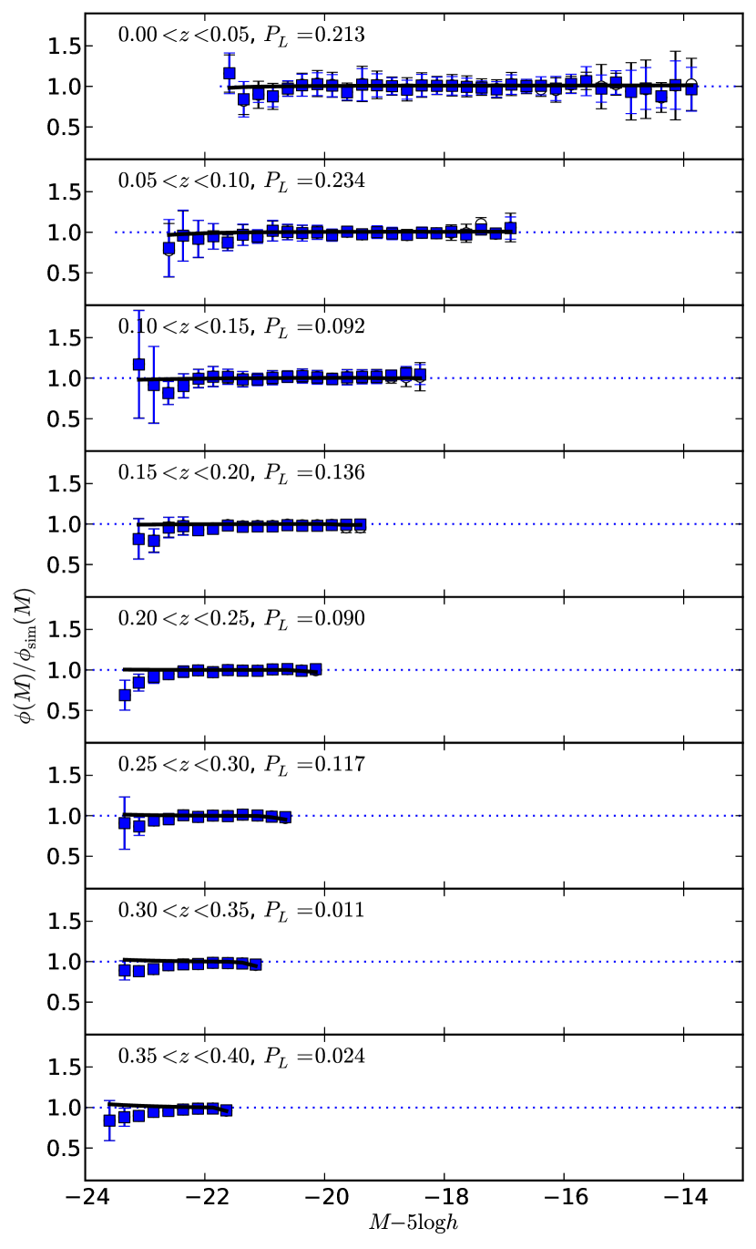
Eight independent mock catalogues were generated for each of two different input LFs, as described above, and used as input catalogues for our LF estimation code. Naturally, when analysing these simulations, we assume a consistent cosmology in calculating distances, apparent magnitudes and volumes.
The Schechter function parameters recovered by the parametric LF estimator, for both non-evolving and pure luminosity evolution simulations, are given in Table 7. In both cases we recover the true LF parameters with minimal bias, at worst.
Fig. 21 shows the LF recovered in eight redshift slices from our evolving mock catalogues. In order to amplify any discrepancies, all estimates have been normalised by the true LF, obtained by substituting the input LF parameters into equation (21). We only plot binned estimates when there is at least one galaxy in that magnitude bin in all eight realisations in order to avoid biasing the mean high if only realisations with one or more galaxies are included or biasing it low if all realisations are used. This eliminates bins fainter than mag, for which galaxies are only found in a subset of the simulations.
For the low redshift () slice, all estimates are in good agreement with the true LF. Faintwards of mag, the scatter in estimates starts to increase due to density variations induced by large-scale structure. The SWML estimator, being insensitive to density variations, has smaller error bars at the faint end.
For the higher redshift slices, we see that and SWML estimators give essentially identical results. There is a tendency for both of these binned estimates to slightly underestimate the bright end of the LF, a consequence of that fact that both binned estimates, unlike our parametric fit, make the assumption that the LF is independent of redshift. Even dividing the simulation into eight redshift slices of width , there is a systematic change of across each slice in these simulations. With broader redshift slices the discrepancy worsens. For example, with , the likelihood ratio probabilities are below 0.001 for the three higher redshift slices. It is likely that our binned estimates of the GAMA LF (Section 4) are biased in a similar fashion. Note that Cole (2011) has recently proposed a method for estimating binned LFs whilst simultaneously fitting for luminosity and density evolution.
Fig. 22 shows the LD estimated from the evolving simulations. The recovered LD, both in redshift bins, equation (16), and as predicted by the parametric fit, equation (14), is in excellent agreement with the prediction given the simulation parameters. The decreasing errors at higher redshift indicate that sample variance is the largest contributing factor to errors in LD for these simulations. This is not the case with the observed LD (Section 4.5), where the dominant source of error, particularly for the and bands, is the applicability of the evolution model (equation 5).