Correlated multiplexity and connectivity of multiplex random networks

Abstract

Nodes in a complex networked system often engage in more than one type of interactions among them; they form a multiplex network with multiple types of links. In real-world complex systems, a node’s degree for one type of links and that for the other are not randomly distributed but correlated, which we term correlated multiplexity. In this paper we study a simple model of multiplex random networks and demonstrate that the correlated multiplexity can drastically affect the properties of giant component in the network. Specifically, when the degrees of a node for different interactions in a duplex Erdős-Rényi network are maximally correlated, the network contains the giant component for any nonzero link densities. On the contrary, when the degrees of a node are maximally anti-correlated, the emergence of giant component is significantly delayed, yet the entire network becomes connected into a single component at a finite link density. We also discuss the mixing patterns and the cases with imperfect correlated multiplexity.

1 Introduction

In the last decade, network has proved to be a useful framework to model structural complexity of complex systems [1, 2]. By abstracting a complex system into nodes (constituents) and links (interactions between them), the resulting graph could be efficiently treated analytically and numerically, through which a large body of new physics of complex systems has been acquired [3, 4, 5]. Most studies until recently have focused on the properties of isolated, single networks where nodes interact with a single type of links. In most, if not all, real-world complex systems, however, nodes in the system can engage in more than one type of interactions or links; People in a society interact via their friendship, family relationship, and/or more formal work-related links, etc. Countries in the global economic system interact via various financial and political channels ranging from commodity trade to political alliance. Even proteins in a cell participate in multiple layers of interactions and regulations, from transcriptional regulations and metabolic synthesis to signaling. Therefore, a more complete description of complex systems would be the multiplex network [6] with more than one types of links connecting nodes in the network. Multiplexity can also have impact on network dynamics; many dynamic processes occurring in complex network systems such as behavioral cascade in social networks [7] or dynamics of systemic risk in the global economic system [8] should be properly understood from the perspective of multiplex network dynamics. Since its introduction in the social network literature [6], however, only a handful of earlier related studies have existed in the physics literature, notably Refs. [9, 10, 11], and the understanding of generic effects of multiplexity remained lacking.

More recently, related concepts such as interacting networks [12] and interdependent networks [13] have been introduced and studied. Leicht and D’Souza [12] studied what they called interacting networks, in which two networks are coupled via inter-network edges, and developed a generating function formalism to study their percolation properties. Buldyrev et al. [13] studied the interdependent networks, in which mutual connectivity in two network layers plays an important role, and found that catastrophic cascades of failure can occur due to the interdependency. Although the specific contexts are different in these studies, if one regards each type of links in a multiplex network to constitute a network layer, and the multiplex network as multilayer network, the multiplex networks and the interacting or interdependent networks may be described by a similar framework at the mathematical level. In this sense, these studies have provided a pioneering insight relevant to multiplex networks that there can be nontrivial effects of having more than one type of links, or channel of interactions, in networks [14, 15].

In Refs. [12, 13], network layers were coupled in an uncorrelated way, in the sense that the connections or pairings between nodes in different layers are taken to be random. In real-world complex systems, however, nonrandom structure in network multiplexity can be significant. For example, a person with many links in the friendship layer is likely to also have many links in another social network layer, being a friendly person. Such a nonrandom, or correlated multiplexity has recently been observed in the large-scale social network analysis of online game community [16], in the world trade system [17], and in transportation network systems [18, 19], and its impact on network robustness has been studied [18, 20]. In this paper, our main goal is to understand the generic role of correlated multiplexity in multiplex system’s connectivity structure.

2 Model and formalism

Figure 1: Schematic illustration of multiplex ER networks with three kinds of multiplex couplings discussed in the text. MP (MN) stands for maximally-positive (maximally-negative) correlated multiplexity.

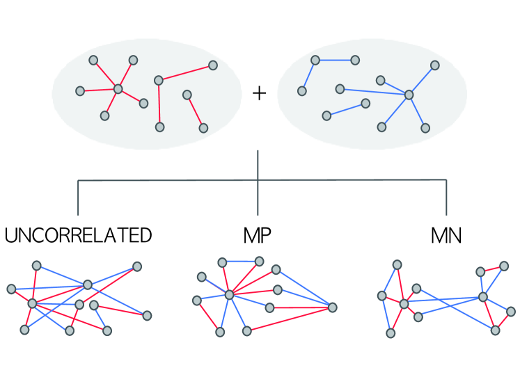
To study how the network connectivity is affected by correlated multiplexity, we consider the following model of multiplex networks with two layers, or duplex networks. The network has $N$ nodes connected by two kinds of links, modeling, for example, individuals participating in two different social interaction channels. We refer the subnetwork formed by each kind of links to as the network layer. Each network layer $l$ ($l=1,2$) is specified by the intralayer degree distribution $\pi^{(l)}(k_{l})$, where degree $k_{l}$ is the number of links within the specific layer $l$ of a node. The complete multiplex network can be specified by the joint distribution $\Pi(k_{1},k_{2})$ or the conditional degree distribution $\Pi(k_{2}|k_{1})$. Generalization into $l>2$ layers is straightforward.

The total degree of a node in the multiplex network is given by $k=k_{1}+k_{2}-k_{o}$, where $k_{o}$ denotes the number of overlapped links in the two layers, which can be neglected in the $N\to\infty$ limit for random, sparse networks with largest degree of at most order ${\cal O}(\sqrt{N})$ [21]. One can obtain the total degree distribution $P(k)$ from the joint degree distribution or the conditional degree distribution as $P(k)=\sum_{k_{1},k_{2}}\Pi(k_{1},k_{2})\delta_{k,k_{1}+k_{2}}=\sum_{k_{1}}\Pi(k-k_{1}|k_{1})\pi^{(1)}(k_{1})$, where $\delta$ denotes Kronecker delta symbol. From $P(k)$, one can follow the standard generating function technique [22] to study the network structure: The generating function $g_{0}(x)$ of the degree distribution $P(k)$ of the mutiplex network can be written as

$$g_{0}(x)=\sum_{k=0}^{\infty}P(k)x^{k}=\sum_{k_{1},k_{2}}\Pi(k_{1},k_{2})x^{k_{1}+k_{2}}~{}.$$ (1)

Emergence of the giant component spanning a finite fraction of the network signals the establishment of connectivity. Size of the giant component $S$ is obtained via

$$S=1-g_{0}(u)=1-\sum_{k=0}^{\infty}P(k)u^{k},$$ (2)

where $u$ is the smallest root of the equation $x=g^{\prime}_{0}(x)/g^{\prime}_{0}(1)\equiv g_{1}(x)$, that is,

$$u=\frac{1}{\langle k\rangle}\sum_{k=1}^{\infty}kP(k)u^{k-1}.$$ (3)

Mean size of the component to which a randomly chosen vertex belongs, $\langle s\rangle$, plays the role of susceptibility and is given by

$$\langle s\rangle=1+\frac{g^{\prime}_{0}(1)u^{2}}{g_{0}(u)[1-g^{\prime}_{1}(u)]}~{}.$$ (4)

The condition for existence of the giant component (that is, $S>0$) is given by the existence of a nontrivial solution $u<1$, leading to the so-called Molloy-Reed criterion [22, 24, 25],

$$\sum_{k}k(k-2)P(k)=\langle k^{2}\rangle-2\langle k\rangle>0~{}.$$ (5)

It is worthwhile to note the related recent generalizations of the generating function method for interacting [12] and interdependent networks [23].

For a multiplex network system, the total degree distribution $P(k)$ is determined from the joint degree distribution $\Pi(k_{1},k_{2})$, which depends on the pattern of correlated multiplexity. Therefore, the presence of correlated multiplexity affects the multiplex system’s connectivity (figure 1). In the following, we specifically consider duplex networks of two Erdős-Rényi (ER) layers [26] and three limiting cases of correlated multiplexity. Using analytical treatment with mean-field-like approximation as well as extensive numerical simulations, we present how the correlated multiplexity can affect the emergence of the giant component in the multiplex system. Similar procedures can also be applied to multiplex scale-free network models [27].

3 Degree distributions

Figure 2: (a) Schematic illustrations of how the mean-field-like calculation for degree distribution is done. (b, c) Degree distributions of interlaced multiplex ER networks with $z_{1}=z_{2}=0.7$ (b) and $z_{1}=z_{2}=1.4$ (c). Points are numerical simulation results for the uncorrelated ($\circ$), MP ($\Box$), and MN ($\diamond$) cases, together with lines representing predictions of mean-field-like calculations.

3.1 Uncorrelated multiplexity

In the absence of correlation between network layers, the joint degree distribution factorizes, $\Pi_{uncorr}(k_{1},k_{2})=\pi^{(1)}(k_{1})\pi^{(2)}(k_{2})$. The total degree distribution of the multiplex network is given by the convolution of $\pi^{(l)}(k_{l})$, $P_{uncorr}(k)=\sum_{k_{1}=0}^{k}\pi^{(1)}(k_{1})\pi^{(2)}(k-k_{1})$, and its generating function $g_{0}^{uncorr}(x)=g_{0}^{(1)}(x)g_{0}^{(2)}(x)$, where $g_{0}^{(l)}(x)$ is the generating function of $\pi^{(l)}(k_{l})$. Using $g_{0}(x)=e^{z(x-1)}$ for the ER network with mean degree $z$, we have $g_{0}^{uncorr}(x)=e^{(z_{1}+z_{2})(x-1)}$ for the duplex ER network with mean intralayer degrees $z_{1}$ and $z_{2}$, which is nothing but the generating function of an ER network with mean degree $z_{1}+z_{2}$. Therefore, we have

$$P(k)=\frac{e^{-z}z^{k}}{k!}$$ (6)

with $z=z_{1}+z_{2}$.

3.2 Maximally-positive correlated multiplexity

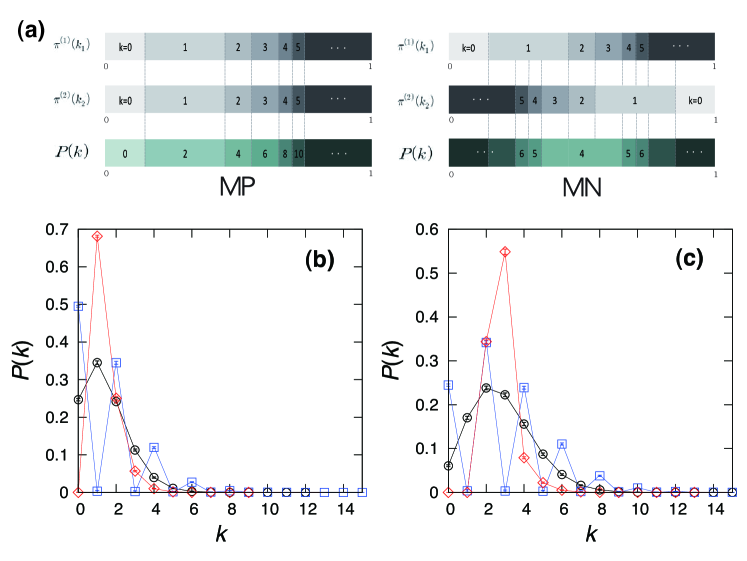
In the maximally-positive (MP) correlated multiplex case, a node’s degrees in different layers are maximally correlated in their degree order; the node that is hub in one layer is also the hub in the other layers, and the node that has the smallest degree in one layer also has the smallest degree in other layers. To obtain the total degree distribution $P(k)$ of the multiplex network, we use the following mean-field-like scheme ignoring fluctuations in the thermodynamic limit ($N\to\infty$), illustrated for the duplex case in figure 2(a). We partition the unit interval into bins of sizes $\pi^{(\ell)}(k_{\ell})$ sorted in order of $k_{\ell}$ for each $\ell$. Combining the two partitions, we have a new partition which can be used to reconstruct $P(k)$ as illustrated in figure 2(a).

3.3 Maximally-negative correlated multiplexity

In the maximally-negative (MN) correlated multiplex case, a node’s degrees in different layers are maximally anti-correlated in their degree order; a node that is hub in one layer has the smallest degree in the other layer, etc. The mean-field-like scheme for duplex case proceeds in a similar way as the MP case, except that we use two partitions sorted in opposite orders respectively as illustrated in figure 2(a).

Figure 3: (a) The giant component size $S$ and (b) the susceptibility $\langle s\rangle$ as a function of the single-layer mean degree $z_{1}$ of the two-layer multiplex ER networks with equal mean layer degrees for uncorrelated (black), MP (blue), and MN (red) cases. Lines represent the solutions of (2) and (4) under the mean-field scheme and symbols represent the numerical simulation results obtained from networks of size $N=10^{4}$ with $10^{4}$ different configurations for the uncorrelated ($\circ$), MP ($\Box$), and MN ($\diamond$) cases. Errorbars denote standard deviations. Gray shade denotes the region in which $S=1$ for the MN case ($z_{1}>z^{*}=1.14619322...$).

4 Duplex ER networks with equal link densities

In this section we consider ER networks with two layers of equal link densities, for which the degree distributions are most easily calculated.

4.1 Uncorrelated case

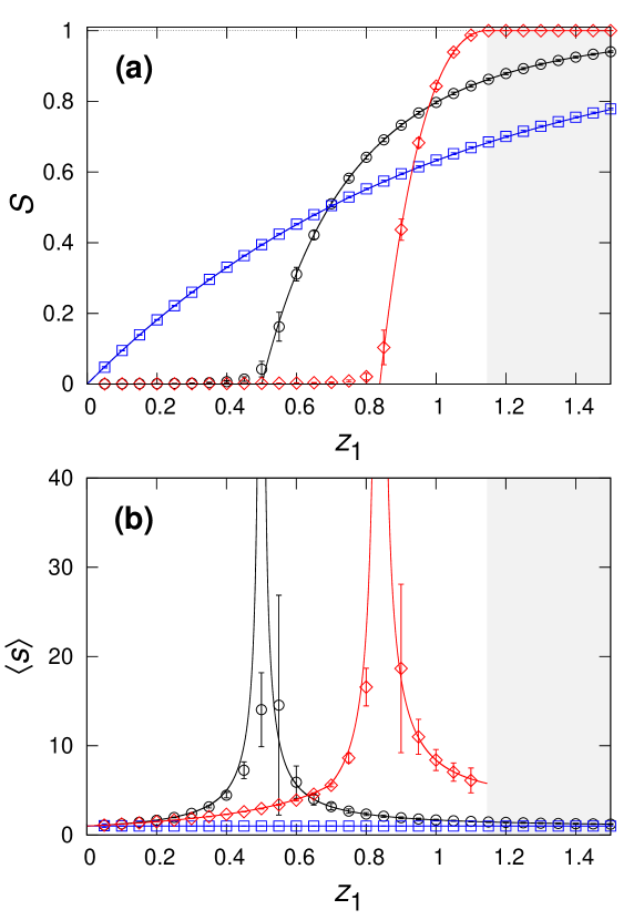
The uncorrelated multiplex ER network is simply another ER network with mean degree $z=2z_{1}$, where $z_{1}$ is the mean degree of the first network layer. The joint degree distribution factorizes, thus the conditional degree distribution $\Pi(k_{2}|k_{1})$ is independent of $k_{1}$ and $\Pi(k_{2}|k_{1})=\pi(k_{2})$, where $\pi(k)$ denotes the Poisson distribution with mean degree $z_{1}$. As we increase $z_{1}$, we have a second-order percolation transition at the critical mean intralayer degree $z_{c}=1/2$ [22, 26], at which the giant component emerges in the duplex network. Giant component size scales in the vicinity of $z_{c}$ as $S\sim(z_{1}-z_{c})^{\beta}$ with $\beta=1$, and the susceptibility as $\langle s\rangle\sim|z_{1}-z_{c}|^{-\gamma}$ with $\gamma=1$, following the standard mean-field critical behaviors [22].

4.2 MP case

In this case, in the mean-field-like scheme ($N\to\infty$) each node has exactly the same degrees in both layers, so the conditional degree distribution becomes $\Pi(k_{2}|k_{1})=\delta_{k_{2},k_{1}}$. Thus we have the degree distribution of the duplex network as

$$P(k)=\left\{\begin{array}[]{ll}e^{-z_{1}}z_{1}^{k/2}/(k/2)!&(k~{}\textrm{even}),\\ 0&(k~{}\textrm{odd}).\end{array}\right.$$ (7)

Therefore, the Molloy-Reed criterion is fulfilled for all nonzero $z_{1}$, as $\langle k^{2}\rangle-2\langle k\rangle=4(z_{1}+z_{1}^{2})-2(2z_{1})=4z_{1}^{2}>0$ for $z_{1}\neq 0$. This means that the giant component exists for any nonzero link density, that is,

$$z_{c}^{MP}=0.$$ (8)

In fact, one can obtain the solution of $S$ and $\langle s\rangle$ explicitly in this case: As $P(k)=0$ for odd $k$, (3) has $u=0$ as a nontrivial solution, from which it follows from (2)

$$S=1-P(0)=1-e^{-z_{1}},$$ (9)

which grows linearly with the link density near origin as $S\sim z_{1}$, that is $\beta=1$. From $u=0$, the susceptibility $\langle s\rangle=1$ for all $z_{1}>0$. This means that only isolated nodes are outside the giant component and all the linked nodes form a single giant component. All these predictions are confirmed by numerical simulations (figure 3).

4.3 MN case

In this case one can easily show that distinct regimes appear as $z_{1}$ increases. Among them, three regimes are of relevance for the giant component properties: i) For $0\leq z_{1}\leq\ln 2$, more than half of nodes are of degree zero in each layer so every linked node in one layer is coupled with a degree-$0$ node in the other layer under MN coupling. In this regime the conditional degree distribution takes a rather complicated form

$$\Pi(k_{2}|k_{1})=\left\{\begin{array}[]{ll}\left[2\pi(0)-1\right]/\pi(0)&(k_{2}=0,k_{1}=0),\\ \pi(k_{2})/\pi(0)&(k_{2}\neq 0,k_{1}=0),\\ \delta_{k_{2},0}&(k_{1}\neq 0),\end{array}\right.$$ (10)

and thus $P(k)$ is given by

$$P(k)=\left\{\begin{array}[]{ll}2\pi(0)-1&(k=0),\\ 2\pi(k)&(k\geq 1).\end{array}\right.$$ (11)

In this regime there is no giant component. ii) For $\ln 2\leq z_{1}\leq z^{*}$, similar consideration leads to $\Pi(k_{2}|k_{1})$ and $P(k)$ given by

$$\Pi(k_{2}|0)=\left\{\begin{array}[]{ll}0&(k_{2}=0),\\ \left[2\pi(0)+\pi(1)-1\right]/\pi(0)&(k_{2}=1),\\ \pi(k_{2})/\pi(0)&(k_{2}\geq 2),\end{array}\right.$$ (12a)

$$\Pi(k_{2}|1)=\left\{\begin{array}[]{ll}\left[2\pi(0)+\pi(1)-1\right]/\pi(1)&(k_{2}=0),\\ \left[1-2\pi(0)\right]/\pi(1)&(k_{2}=1),\\ 0&(k_{2}\geq 2),\end{array}\right.$$ (12b)

$$\Pi(k_{2}|k_{1})=\delta_{k_{2},0}\qquad\qquad\qquad\qquad(k_{1}\geq 2),$$ (12c)

and

$$P(k)=\left\{\begin{array}[]{ll}0&(k=0),\\ 2[2\pi(0)+\pi(1)-1]&(k=1),\\ 2\pi(2)-2\pi(0)+1&(k=2),\\ 2\pi(k)&(k\geq 3).\end{array}\right.$$ (12m)

In this regime, $\langle k^{2}\rangle-2\langle k\rangle=2(z_{1}^{2}-z_{1}-2e^{-z_{1}}+1)$, which becomes positive for $z_{1}>z_{c}^{MN}$ where

$$z_{c}^{MN}=0.838587497...$$ (12n)

Therefore the giant component emerges at a significantly higher link density than the uncorrelated multiplex case. Being delayed in its birth, the giant component grows more abruptly once formed [see figure 3(a)] than the other two cases. This regime is terminated at $z=z^{*}$, determined by the condition $2\pi(0)+\pi(1)=1$, from which we have $z^{*}=1.14619322...$ iii) For $z_{1}\geq z^{*}$, we have $P(0)=P(1)=0$. In that case, we have $u=0$ from (3) and thereby $S=1$ from (2). This means that the entire network becomes connected into a single component at this finite link density, which can never be achieved for ordinary ER networks. Despite these abnormal behaviors and apparent differences in the steepness of the order parameter curve near $z_{c}$, the critical behavior is found to be consistent with that of standard mean-field, $\beta=1$ and $\gamma=1$ (figure 4).

5 Imperfect correlated multiplexity

In the previous section we have seen that maximally correlated or anti-correlated multiplexity affects the onset of emergence of giant component in multiplex ER networks. Despite its mathematical simplicity and tractability, in real-world multiplex systems the correlated multiplexity would hardly be maximal. Therefore it is informative to see how the results obtained for the maximally correlated multiplexity are interpolated when the system possesses partially correlated multiplexity.

Figure 5: Plot of equation (15) for the critical mean degree $z_{c}$ as a function of $q$, the fraction of correlated multipex nodes. The cases $q=1$ denote maximally correlated multiplexity, $0<q<1$ partially correlated multiplexity, and $q=0$ uncorrelated multiplextiy. The vertical dotted line is drawn at $q=2-1/\ln 2$ across which $z_{c}$ takes different formulae in equation (15b).

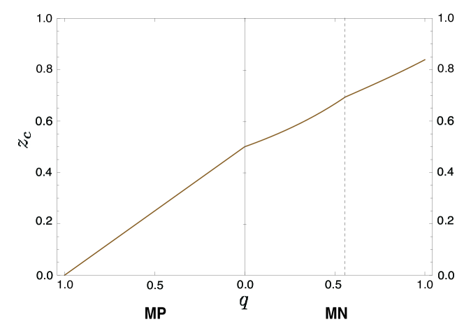
To this end, we consider duplex ER networks where a fraction $q$ of nodes are maximally correlated multiplex while the rest fraction $1-q$ are randomly multiplex. Then the degree distribution of the interlaced network is given by $P_{partial}(k)=qP_{maximal}(k)+(1-q)P_{uncorr}(k)$, where $maximal$ is either $MP$ or $MN$. Following similar steps as in the previous section we obtain the critical link density as a function of $q$ as

$$z_{c}=(1-q)/2$$ (12oa)

for positively correlated case and

$$z_{c}=\left\{\begin{array}[]{ll}1/(2-q)&\textrm{\qquad$(q<2-1/\ln 2)$},\\ z_{1}(q)&\textrm{\qquad$(q>2-1/\ln 2)$}\end{array}\right.$$ (12ob)

for negatively correlated case, where $z_{1}(q)$ is the solution of $(2-q)z_{1}^{2}-z_{1}-2qe^{-z_{1}}+q=0$. In figure 5, we show the plot of $z_{c}$ as a function of $q$ given by (15). This result shows that the effect of correlated multiplexity is not only present for maximally correlated cases but for general $q$.

6 Duplex ER networks with general link densities

In the previous sections we focused on the cases with $z_{1}=z_{2}$. In this section we consider general duplex ER networks with $z_{1}\neq z_{2}$. We performed numerical simulations with $N=10^{4}$ for MP, uncorrelated, and MN correlated multiplex cases with $z_{1}$ and $z_{2}$ in the range from $0$ to $3$. In figure 6, the giant component size $S$ for general $z_{1}$ and $z_{2}$ are shown. Similarly to the $z_{1}=z_{2}$ cases, the giant component emerges at lower link densities for the MP case but grows more slowly than the uncorrelated case, whereas it emerges at higher link densities for the MN case but grows more abruptly and connects all the nodes in the network at finite link density. Therefore the effect of correlated multiplexity is qualitatively the same and generic.

Figure 6: Numerical simulation results of the size of giant component of duplex ER networks with (a) MP, (b) uncorrelated, and (c) MN cases. In (d–f), the giant component size $S$ (red) is plotted for $z_{2}=0.4$, along with the assortativity coefficient $r$ (blue) for the MP (d), uncorrelated (e), and MN (f) cases. Mean-field-like calculation results (lines) deviates from the numerical simulation results ($\circ$) when assortativity coefficient ($\Box$) becomes nonzero, that is, the network display degree-degree correlation. Errorbars denote standard deviations from $10^{4}$ independent runs.

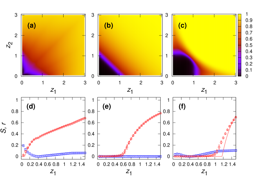
It is worthwhile to note, however, that although the mean-field-like approximation for $P(k)$ introduced in section 3, which was very effective for equal link densities, still yields a qualitatively correct picture, it fails in quantitative agreement with numerical simulation results for general $z_{1}\neq z_{2}$. To understand the origin of this discrepancy, we consider network correlations. Assortativity coefficient $r$ [28] defined as the Pearson correlation coefficient between the (total) degrees of nodes connected by a link in the network measures the degree-degree correlations in the network at the two-node level. Nonzero assortativity is known to alter the connectivity properties of networks [28]. To see the role of degree-degree correlations induced by correlated multiplexity, in figure 6(d–f) we plot the giant component size obtained from numerical simulations and mean-field calculations, together with the assortativity coefficient as a function $z_{1}$ with $z_{2}=0.4$ fixed. With uncorrelated multiplexity, the degree-degree correlation is absent, $r=0$, and the numerical simulation and mean-field calculation agree perfectly [figure 6(e)]. For MP and MN cases, however, the assortativity of multiplex network is generically nonzero (positive), that is the multiplex network becomes correlated, which is responsible for the deviations between the numerical simulation and mean-field calculation results. This discrepancy vanishes at $z_{1}=z_{2}$, at which the assortativity also vanishes [figures 6(d,f)]. Note that there was no degree-degree correlations at the individual network layer level. Therefore this result shows that generically correlated multiplexity not only modulate $P(k)$ but also introduce higher-order correlations in the multiplex network structure. Meanwhile, it is worthwhile to note that such a multiplexity-induced degree correlation has similar origin as the correlation in colored-edge networks recently studied in a different context of network clustering [29].

7 Conclusion

In conclusion, we have studied the effect of correlated multiplexity on the structural properties of multiplex network system, a better representation of most real-world complex systems than the single, or simplex, network. We have demonstrated that the correlated multiplexity can dramatically change the giant component properties. With positively correlated multiplexity, the giant component emerges at a much lower critical link density, which even approaches to zero for MP case, than for uncorrelated multiplex cases. Once formed, however, the giant component grows much more gradually. With negatively correlated multiplexity, the giant component emerges at a much higher critical density than for uncorrelated multiplex cases, but once formed it grows more abruptly and can establish the full connectivity to connect the entire network into a single component at a finite link density. These results show that a multiplex complex system can exhibit structural properties that cannot be represented by its individual network layer’s properties alone, the impact of which on network dynamics is to be explored in future study.

References

- [1] Watts D J and Strogatz S H 1998 Nature 393 440
- [2] Barabási A-L and Albert R 1999 Science 286 509
- [3] Caldarelli G 2007 Scale-free networks (Oxford University Press, Oxford)
- [4] Newman M E J 2010 Networks (Oxford University Press, Oxford)
- [5] Havlin S and Cohen R 2010 Complex neworks (Cambridge Unviersity Press, Cambridge).
- [6] Wasserman S and Faust K 1994 Social network analysis (Cambridge University Press, Cambridge).
- [7] Brummitt C D, Lee K-M, Goh K-I 2011 arXiv:1112.0093.
- [8] Lee K-M, Yang J-S, Kim G, Lee J, Goh K-I and Kim I-M 2011 PLoS ONE 6 e18443
- [9] Soderberg B 2003 Phys Rev E 68 015102
- [10] Kim D-H, Kahng B and Kim D 2004 Eur Phys J B 38 305
- [11] Kurant M and Thiran P 2006 Phys Rev Lett 96 138701
- [12] Leicht E A and D’Souza R M 2009 arXiv:0907.0894
- [13] Buldyrev S V, Parshani R, Paul G, Stanley H E and Havlin S 2010 Nature 464 1025
- [14] Parshani R, Buldyrev S V and Havlin S 2011 Proc Natl Acad Sci USA 108 1007
- [15] Brummitt C D, D’Souza R M and Leicht E A 2011 arXiv:1106.4499
- [16] Szell M, Lambiotte R and Thurner S 2010 Proc Natl Acad Sci USA 107 13636
- [17] Barigozzi M, Fagiolo G and Garlaschelli D 2010 Phys Rev E 81 046104
- [18] Parshani R, Rozenblat C, Ietri D, Ducruet C and Havlin S 2010 EPL 92 68002
- [19] Xu X-L, Qu Y-Q, Guan S, Jiang Y-M and He D-R 2011 EPL 93 68002
- [20] Buldyrev S V, Shere N and Cwilich G A 2011 Phys Rev E 83 016112
- [21] Nakata T 2008 Stat Prob Lett 78 1929
- [22] Newman M E J, Strogatz S H and Watts D J 2001 Phys Rev E 64 026118
- [23] Son S-W, Bizhani G, Christensen C, Grassberger P, Paczuski M 2012 EPL 97 16006
- [24] Molloy M and Reed B 1995 Random Struct Algorithms 6 161
- [25] Cohen R, Erez K, ben-Avraham D and Havlin S 2000 Phys Rev Lett 85 4626
- [26] Erdős P and Rényi A 1960 Publ Math Inst Hung Acad Sci 5 17
- [27] Goh K-I, Kahng B and Kim D 2001 Phys Rev Lett 87 278701
- [28] Newman M E J 2002 Phys Rev Lett 89 208701
- [29] Gleeson J P, Melnik S and Hackett A 2010 Phys Rev E 81 066114