Evidence for a Phase Transition
in 2D Causal Set Quantum Gravity
Abstract
We present evidence for a phase transition in a theory of 2D causal set quantum gravity which contains a dimensionless non-locality parameter . The transition is between a continuum phase and a crystalline phase, characterised by a set of covariant observables. For a fixed size of the causal set the transition temperature decreases monotonotically with . The line of phase transitions in the v/s plane asymptotes to the infinite temperature axis, suggesting that the continuum phase survives the analytic continuation.
Causal set theory(CST) is a discrete approach to quantum gravity which combines local Lorentz invariance with a fundamental discreteness [1]. The spacetime continuum is replaced by a locally finite poset or causal set, with the order relation being the analog of the spacetime causal order. The continuum quantum gravity path integral is thus replaced by a discrete sum over causal sets
| (1) |
where is a sample space of causal sets and is an appropriately chosen action. The combination of local Lorentz invariance with fundamental discreteness gives rise to a non-locality in the continuum approximation, making the extraction of local geometric data highly non-trivial. The recent construction of a discrete Einstein-Hilbert action, the Benincasa-Dowker action for causal sets [2], thus allows us for the first time to begin a serious study of the causal set partition function .
Apart from a choice of action, also depends crucially on the sample space . A natural starting choice for is the collection of countable causal sets; in classical sequential growth models of causal sets, for example, is further restricted to causal sets that are past finite [3, 4]. The collection of -element causal sets is known to be strongly dominated by the “Kleitman-Rothschild”(KR) class of causal sets in the large limit. These are of a fixed time extent with only three “moments of time”, and admit no continuum approximation [5]. This presents a potential “entropy problem” in CST. In order to be able to recover spacetime-like behaviour, therefore, the causal set action, or more generally the choice of dynamics, should be able to counter this entropy. Indeed, classical sequential growth dynamics is an example in which the KR entropy is made sub-dominant by the dynamics [3].
In this work we consider a two dimensional theory of causal sets, defined by the 2-dimensional Benincasa-Dowker action [2], and an order theoretic dimensional restriction of to , the set of -element “2D orders”, defined as follows. Let and , , with , , for . and are then total orders with given by the natural ordering in : for every pair either or , and similarly for . An -element 2D order is the intersection of two total -element orders and , i.e., in iff and . A useful example of an -element 2D order is a set of events in 2d Minkowski spacetime ordered by causality, and such that in light cone coordinates , and for .
The motivation for restricting the sample space to stems from the fact that the causal set discretisation of a conformally flat, topologically trivial 2d spacetime is a 2D order [6]. However, not all 2D orders can be approximated by continuum spacetimes. This means that the choice of corresponds only to a restriction of poset dimension and not spacetime dimension. Moreover, only in a very limited sense do these dimensions coincide: every 2D order admits an order preserving embedding into a patch of 2d Minkowski spacetime , i.e., for every in , causally precedes in . Such an embedding though necessary, is not sufficient to ensure a continuum approximation for .
A striking feature of 2D orders is that in the asymptotic limit , is dominated by “random” 2D orders, namely those approximated by Minkowski spacetime [6, 7, 8]. A random 2D order is the intersection of two total orders and which are chosen randomly and independently from . Hence unlike the unrestricted sample space, spacetime like causal sets dominate the uniform measure on . It is thus of obvious interest to study the effect of on this entropic feature of .
While there is no natural Planck scale in 2D gravity, in CST one requires a volume cut-off in order to realise the continuum approximation, and this plays the role of a fundamental scale. In addition, the 2d Benincasa-Dowker action for a causal set includes a “non-locality” scale required to suppress large fluctuations about the mean in the continuum approximation [2, 9]. can be expressed in terms of the abundances of the “intervals” of fixed cardinality in
| (2) |
where and
| (3) |
Figure 1 shows the typical behaviour of .
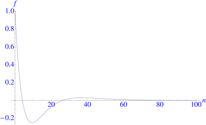
For , , and thus, effectively, the action for a fixed includes the abundance of intervals only upto size . To avoid infrared errors in counting such intervals for finite , should in addition be bounded below by .
The goal of writing down a partition function for quantum gravity is to eventually construct and calculate expectation values of covariant observables. The analog of covariance in causal set theory is label independence, and hence we seek to construct label invariant observables. We have already encountered an example of such an observable, namely, the action . Another important covariant observable is the Myrheim-Myer dimension [10] for a causal set, which in the continuum approximation reproduces the Minkowski spacetime dimension. We will construct several such covariant observables in what follows and use them to determine the existence of a continuum approximation.
However, as we have defined it, the sample space is itself the collection of labelled 2D orders. While every 2D order admits worth of relabellings, each of these relabellings does not produce a distinct labelled 2D order. If is a labelled causal set containing a pair of elements and with the same past and future sets, the relabelling is an automorphism . An extreme example is the antichain or completely unordered set – every relabelling produces the same labelled causal set. Since the action itself is label invariant, the partition function over unlabelled causal sets has an additional weight of for each unlabelled 2D order , where is the cardinality of the Automorphism group of a labelled counterpart. While it is possible to view this additional measure as a “quantisation ambiguity”, it should be stressed that the observables that we construct are nevertheless strictly covariant.
An approach to evaluating the expectation values of covariant observables is to Euclideanise the partition function, in the process converting the quantum system into a thermodynamic one. Replacing the set of Lorentzian metrics wholesale for Euclidean ones, however, makes little of the importance of causal structure, and moreover, can lead to highly fractal, non-manifold like behaviour [11]. Instead, as suggested in [12] one can transition to a thermodynamic partition function by introducing a new parameter into the action and taking . This leaves the sample space unchanged and hence there is no ambiguity in the interpretation of the covariant thermodynamic results. A similar “parameter-based” analytic continuation employed in the causal dynamical triangulation approach, on the other hand, does lead to a Euclideanisation of the sample space itself [13].
For concreteness, we adopt the following prescription. Namely, we replace the complex weights with , and obtain the thermodynamic partition function by taking :
| (4) |
The limit is the uniform distribution, dominated by the 2D random orders, approximated by an interval in Minkowski spacetime for finite . As , since the action is not positive definite, causal sets with the largest negative values of the action should dominate, modulo entropic effects. Thus, one expects a cross-over at finite .
In this work, we use Markov Chain Monte Carlo(MCMC) methods to study this partition function. The results we present are the first in a larger effort to study causal set quantum dynamics using MCMC techniques [14]. The restriction to 2 dimensions leads to a substantial simplification which translates into rapid mixing or thermalisation of the Markov Chain. Our simulations are carried out for relatively small causal sets () but this is sufficient to show emergent continuum behaviour. One of the main observations of our present work is the existence of a phase transition at finite , rather than the cross-over suggested above. The transition is from a continuum-like phase to a crysalline non-continuum phase, and is well characterised by the change in the expectation values of a set of covariant observables.
We first briefly review the basics of causal set theory, and refer the reader to [15] for more detail. A causal set is a locally finite partially ordered set (poset), i.e., a countable collection of elements with an order relation which is (i) transitive (), (ii) irreflexive, () and (iii) locally finite, i.e., if and then the cardinality of the set is finite. We say that two elements are linked if and there is no such that . Local finiteness implements the physical requirement of a fundamental spacetime discreteness: a finite spacetime volume contains only a finite number of “spacetime atoms”. A continuum spacetime is said to be an approximation to an underlying discrete causal set for a spacetime volume “cut-off” , if there exists an embedding which is (i) order preserving: for , , and (ii) is a Poisson distribution of events in :
| (5) |
is the probability of finding elements of in a spacetime volume . Conversely, one can generate a causal set from via a Poisson sprinkling, with induced by for the sprinkled points. A causal set generated this way is therefore not a regular lattice but a “random lattice”. Starting with a sample space of finite element causal sets , the thermodynamic limit does not correspond to the continuum limit of the theory, but rather its infrared limit. This means that a finite cardinality causal set can be well approximated by a region of continuum spacetime without taking the limit.
We construct the MCMC via the exchange move on a 2D order defined as follows. First pick or at random. Wlog, let this be . Next, pick a pair of elements of at random and perform the exchange , while leaving unchanged. The new 2D order then has the new elements and , while all other elements remain the same. It is clear that the move is reversible.
Claim 1.
The exchange move on labelled 2D orders has no fixed points in the space of labelled 2D orders.
Proof: Wlog, let for some . There are three cases to examine: (a) If , then and . Under the exchange while which means that and are now unrelated. (b) Similarly if , then after the exchange the two elements are unrelated. (c) If they are unrelated to start with then either (i) and , in which case after the exchange or (ii) and , in which case after the exchange . In all three cases, therefore the exhange move makes a non-trivial modification to the relationship between the th and th elements, thus giving rise to a new, distinct labelled causal set. ∎
We employ a Metropolis-Hastings algorithm, accepting a move if the difference in the action is negative and rejecting a move only if , where is a random number in . Since each move depends on a pair of elements, we define a sweep to be moves, with the following observables recorded every sweep. (i) The ordering fraction where is the number of relations in the causal set with the maximum number of relations possible; is therefore analogous to the filling fraction in an Ising model. In 2 spacetime dimensions is also the inverse of the Myrheim-Myer dimension. Thus, for flat spacetime, we should expect . (ii) The action : for flat space it was shown in [16] that for and simulations show that this is also true for . (iii) Time Asymmetry: given that the action is itself time-reversal invariant, it is useful to check whether the dynamics preserves this property. A rough measure of time asymmetry is the difference in the number of maximal and minimal elements in the causal set; in flat spacetime . (iv) The height of the causal set or the length of the longest chain. This corresponds in the continuum approximation to the maximum proper time in flat spacetime [17]. (v) The abundances of -element intervals for all . In flat spacetime has a specific monotonic fall off with and this provides a useful comparison.
Our focus in this work is to examine the behaviour of these observables as function of the inverse temperature as one varies the non-locality parameter . We present results for , with a range of values for between and . We perform the simulations for sweeps which translates to million attempted moves.
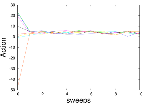
We test for thermalisation starting from several different types of initial 2D orders. Our current algorithm includes the following 8 initial types of causal sets: (i) a randomly labelled chain or totally ordered set (ii) the antichain (iii) a random 2D order, which is approximated by the Minkowski interval (iv-v) two 2D random orders of size each with an intervening element chain or antichain, (vi) two 2D random orders of size N/16 with an intervening antichain of size 7N/8 (vii) two element random orders stacked on top of each other and (viii) a crystalline causal set of the kind we will describe shortly. We find that there is rapid mixing starting from these varied configurations, an example of which is shown in Figure 2.
The expectation values are calculated from a sampling per autocorrelation time . As expected, increases with so that the number of independent samples rapidly decreases for larger .
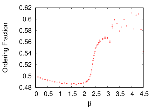
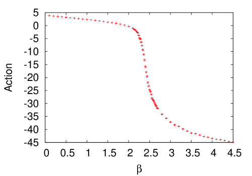
For fixed we find a rapid change in the expectation values of the observables around a fixed suggesting a phase transition as shown in Figure (3). The exact value of can be determined by looking at the behaviour of the autocorrelation times which peak at the same for all observables. For the example shown in Figure 3 it is clear that roughly, . We have included the error bars in the plots, but these are typically very small.
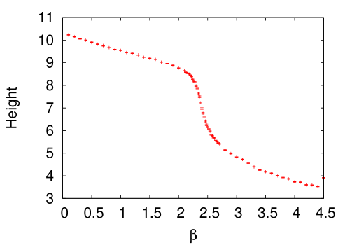
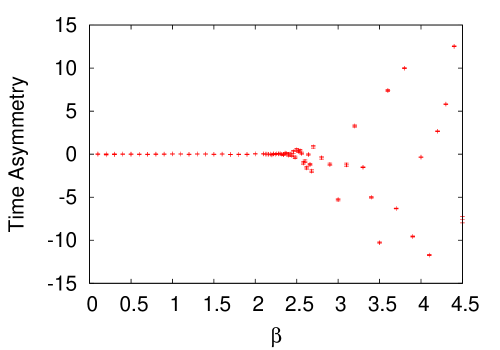
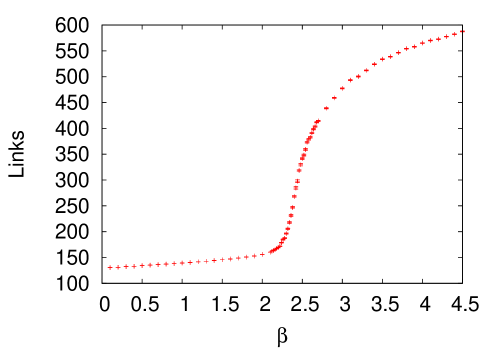
That there is an actual differentiation into two phases becomes explicit on examining the 2D orders themselves. We record the configurations in the Markov Chain every 100 sweeps. For , we find evidence for a “continuum” phase (Phase I), and for , a “crystalline” phase (Phase II). We show examples of configurations in these two phases in Figure 4, where the light cone coordinates have been turned clockwise by for ease of plotting.
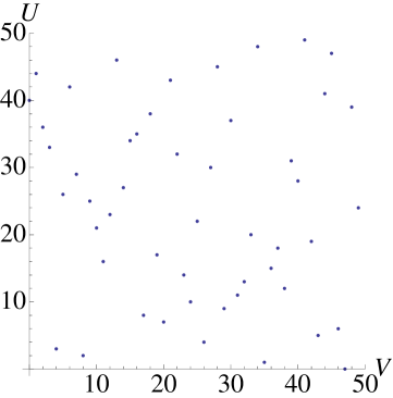
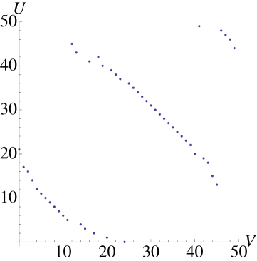
A quick look at a typical causal set from Phase I shows a causal set that resembles a random discretisation of a spacetime. Indeed, the expectation values for a fixed corroborate this. For example for and , (a) ordering fraction: with an error less than , which means that the Myrheim-Myer dimension , (b) height: , which should be compared to the height of a Minkowski interval which is , (c) time asymmetry: and the (d) Action: which should be compared to the residual or boundary value of for Minkowski spacetime [16]. In addition, if we plot the abundance of the intervals of cardinality in and contrast it that for a random 2D order, we find that these match very closely as shown in Figure 5. As nears the transition, the expectation values of these observables gradually change. However, the typical causal set continues to retain the features of a random lattice.
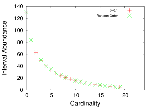
Thus, looking at the explicit values of the observables, it is clear that Phase I corresponds to a continuum phase.
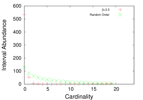
A typical causal set in Phase II on the other hand, has a most unexpected character as shown in Figure 4. It shares some superficial features of a KR causal set, being of limited time extent, but does not strictly belong to this class. It has a regularity, or crystalline nature, suggesting that it does not have a continuum approximation. The values of most observables differ considerably from those in Phase I. For example, for , (a) Ordering Fraction: which gives a fractal dimension for the causal set of , (b) Height: (c) Time Asymmetry: , which is a large deviation from the expected value of zero. This may be the result of a spontaneous breaking of the time symmetry, similar to that in the low temperature phase of the Ising model, but may also be the result of poorer statistics at larger . (d) Action: , i.e., the action tries to take on the lowest possible (negative) value. In contrast to Phase I, the abundances of intervals as shown in Figure 6 is very different from that of Minkowski spacetime. In particular, align themselves with the positive part of and vanish for those for which , thus minimising the action.
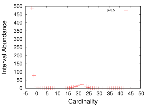
The existence of these distinct phases thus strongly suggest a phase transition. It is tempting to draw the obvious analogy with the Ising model: at high temperatures one has the disordered or random Phase I, while at low temperatures, there is the higly ordered crystalline Phase II which exhibits a spontaneous breaking of symmetry. Although it is difficult at this stage of our work to assess the order of this transition, there are hints that it may be of second order. To begin with, the autocorrelation time peaks at the phase transition as do the fluctuations in the observables. The size of the fluctuations gives us a rough estimate of the temperature of the phase transition, and this coincides with the peak in the autocorrelation time. Moreover, the transitions shown in Figure 3 appear to be smooth. A more conclusive assessment would require a detailed understanding of the dependence of these results on the cardinality .
It is important to stress that while the nature of this phase transition is definitely of interest, it does not play a crucial role in determining continuum behaviour. In other lattice-based approaches in which discretisation is used only a calculational tool, the appearance of a second order phase transition signals the fact that the continuum limit of the theory exists. However, in a fundamentally discrete theory like causal set theory, it is only the continuum approximation we seek, and as we have just seen, this does not depend on the existence and the nature of a phase transition.
More important to our discussion, then is the question of what this thermodynamic calculation can mean for quantum gravity. How much of the above discussion, if any, survives the analytic continuation? As varies in , our simulations show that the phase transition survives, but the critical temperature increases monotonically with . Using the maximal size of the fluctuations to estimate the critical temperature, we plot as a function of . The negative axis corresponds to the region of interest, i.e., the quantum regime, while the positive axis corresponds to the thermodynamic regime to which our above calculations belong. As shown in Figure 7 the line of phase transitions which separates Phase I from Phase II asymptotes to the axis which itself belongs to the continuum Phase I. This strongly suggests that the non-continuum crystalline Phase II is confined to the region and that the continuum phase survives the analytic continuation into the region. The phase diagram also suggests that smaller is in a sense “favoured” by Phase I, which is consistent with having smaller fluctuations in the action and hence a more reliable continuum approximation. A similar type of analysis has been used recently in studying the phase structure of QCD [18].
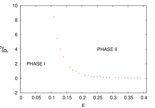
A more careful study of the phase diagram is clearly in order. For example, does the gradual change in the observables in Phase I as one moves towards signal a significant shift away from Minkowski spacetime? In a recent paper [19] the phase structure of the 4d causal dynamical triangulation model of quantum gravity was studied. The phase diagram of this theory includes three phases, two of which, Phase C and Phase B, seem to be at least superficially analogous to our Phases I and II respectively. The phase transition B-C is argued in [19] to be second order and it would be interesting to explore whether these two theories lie in the same universality class.
Since a more ambitious goal is to work with the unrestricted sample space , and an action with at least dimension [14], it is not immediate that 2d CST can teach us straightforward lessons. Nevertheless, our analysis opens a new window into causal sets, and with it a host of questions that can finally begin to be addressed. One of the more interesting of these is whether there is a renormalisation group type analysis with stable fixed points for . This would suggest that the non-locality scale is not a free parameter, but can be determined from the quantum dynamics.
Acknowledgements: I would like to thank Rafael Sorkin, David Rideout, Fay Dowker and Alexei Kurkela for discussions. I am also grateful for the hospitality of the High Energy Theory Group at McGill University where most of this work was carried out. This research was supported in part by an NSERC Discovery grant to the McGill University High Energy Theory Group and an ONR grant to McGill University. The numerical simulations were carried out on a high performance cluster at the Raman Research Institute.
References
- [1] L. Bombelli, J. Lee, D. Meyer, R.D. Sorkin, Phys. Rev. Lett. 59:521-524 (1987).
- [2] D. M. T. Benincasa and F. Dowker, Phys. Rev. Lett. 104, 181301 (2010)
- [3] D. P. Rideout and R. D. Sorkin, Phys. Rev. D 61, 024002 (2000)
- [4] G. Brightwell, H.F. Dowker, R.S. Garcia, J. Henson, R.D. Sorkin, Phys. Rev. D67, 084031, (2003).
- [5] D. Kleitman and B. L. Rothschild, Trans. Am. Math. Soc. 205, 205 (1975).
- [6] G. Brightwell, J. Henson, S. Surya, Class.Quant.Grav.25:105025,2008
- [7] M.H. El-Zahar and N.W. Sauer, Order 5, 239, (1988).
- [8] P. Winkler, Order 7, 329, (1991).
- [9] R. D. Sorkin, “Does locality fail at intermediate length-scales,” In Oriti, D. (ed.): Approaches to quantum gravity* 26-43, [gr-qc/0703099].
- [10] D.A. Meyer, The Dimension of Causal Sets, PhD thesis (M.I.T., 1988).
- [11] R. Loll, Living Rev. Rel. 1, 13 (1998). [gr-qc/9805049].
- [12] R. D. Sorkin, “Is the spacetime metric Euclidean rather than Lorentzian?,” To appear in Recent Research in Quantum Gravity, edited by A. Dasgupta (Nova Science Publishers NY), [arXiv:0911.1479 [gr-qc]].
- [13] J. Ambjorn, J. Jurkiewicz and R. Loll, Phys. Rev. Lett. 93, 131301 (2004)
- [14] Joe Henson, David Rideout and Sumati Surya. Work in progress.
- [15] R.D. Sorkin, Causal Sets: Discrete Gravity (Notes for the Valdivia Summer School), In Proceedings of the Valdivia Summer School, edited by A. Gomberoff and D. Marolf; S. Surya, “Directions in Causal Set Quantum Gravity,” To appear in Recent Research in Quantum Gravity, edited by A. Dasgupta (Nova Science Publishers NY), [arXiv:1103.6272 [gr-qc]].
- [16] D. M. T. Benincasa, F. Dowker, B. Schmitzer, Class. Quant. Grav. 28, 105018 (2011).
- [17] G. Brightwell, R. Gregory, Phys. Rev. Lett. 66:260-263 (1991).
- [18] P. de Forcrand, O. Philipsen, Phys. Rev. Lett. 105, 152001 (2010).
- [19] J. Ambjorn, S. Jordan, J. Jurkiewicz, R. Loll, [arXiv:1108.3932 [hep-th]].