Optimal Control with Reset-Renewable Resources.

R. Takeia,e W. Chenb,f Z. Clawsonc,f S. Kirovd,f  and  A. Vladimirskyb,c,g A Department of Electrical Engineering and Computer Sciences, UC Berkeley, CA 94720 B Department of Mathematics, Cornell University, Ithaca, NY 14853 C Center for Applied Mathematics, Cornell University, Ithaca, NY 14853 D Department of Mathematical Sciences, Carnegie Mellon University, Pittsburgh, PA 15213 E Supported in part by ONR grants N0014-03-1-0071, N00014-07-1-0810, N00014-08-1-1119, DOE grant DE-FG02-05ER25710, an ARO MURI through Rice University and the CHASE MURI grant 556016. F Supported in part by the National Science Foundation through the Research Experiences for Undergraduates Program at Cornell. G Supported in part by the National Science Foundation grant DMS-1016150.
Abstract.

We consider both discrete and continuous control problems constrained by a fixed budget of some resource, which may be renewed upon entering a preferred subset of the state space. In the discrete case, we consider both deterministic and stochastic shortest path problems on graphs with a full budget reset in all preferred nodes. In the continuous case, we derive augmented PDEs of optimal control, which are then solved numerically on the extended state space with a full/instantaneous budget reset on the preferred subset. We introduce an iterative algorithm for solving these problems efficiently. The method’s performance is demonstrated on a range of computational examples, including optimal path planning with constraints on prolonged visibility by a static enemy observer.

In addition, we also develop an algorithm that works on the original state space to solve a related but simpler problem: finding the subsets of the domain “reachable-within-the-budget”.

This manuscript is an extended version of the paper accepted for publication by SIAM J. on Control and Optimization. In the journal version, Section 3 and the Appendix were omitted due to space limitations.

1. Introduction.

Dynamic programming provides a convenient framework for finding provably “optimal” strategies to control both discrete and continuous systems. The optimality is usually defined with respect to a single criterion or cost (e.g., money, fuel, or time needed to implement each particular control). Given a set of possible system configurations ΩΩ\Omega, the value function is defined as the cost of such optimal control for each starting position 𝒙Ω𝒙Ω\mbox{\boldmath${x}$}\in\Omega, and the Dynamic Programming equations are then solved to recover this value function.

Realistic applications usually involve several different criteria for evaluating control strategies and the notion of “optimality” becomes more complicated. One natural approach is to focus on a single “primary” cost to be optimized, while treating all other (“secondary”) costs as constraints. A typical application of this type is to find the fastest path to the target subject to constraints on the maximum use of energy along that path. Another possible constraint is on the maximum total amount of time that a robot can be visible to an unfriendly observer while moving to a target. Kumar and Vladimirsky have recently introduced efficient numerical methods for these and similar constrained-optimal control problems in continuous domains [29]. We will refer to such problems as “budget-constrained” since the original state space will have to be expanded to keep track of the remaining “resource-budget” to satisfy the constraint. (E.g., two different starting energy-budgets may well result in very different “constrained time-optimal” paths, even when the starting physical position is the same.)

This state space expansion leads to a significantly larger system of augmented dynamic programming equations or a higher-dimensional domain in the continuous case. Thus, the computational efficiency of numerical methods becomes particularly important. In many applications it is natural to assume that the resource budgets are non-renewable and that every change in the system state results in an immediate budget decrease. This introduces a natural “causal ordering” on the expanded state space: the knowledge of energy-constrained time-optimal controls for the starting energy-budget 𝒃1subscript𝒃1\mbox{\boldmath${b}$}_{1} can be used in computing such constrained-optimal controls for a higher budget 𝒃2>𝒃1subscript𝒃2subscript𝒃1\mbox{\boldmath${b}$}_{2}>\mbox{\boldmath${b}$}_{1}. The efficiency of methods introduced in [29] hinges on this explicit causality.

In the current paper we focus on a more general situation, where the budget can be instantaneously reset to its maximum value by visiting a special part of the state space 𝒮Ω𝒮Ω\mathcal{S}\subset\Omega and the budget is decreasing when moving through the rest of the state space 𝒰=Ω\𝒮.𝒰\Ω𝒮\mathcal{U}=\Omega\backslash\mathcal{S}. If the limited resource is fuel, 𝒮𝒮\mathcal{S} can be thought of as a discrete set of gas stations. On the other hand, if the secondary cost is the vehicle’s exposure to an unfriendly observer, the 𝒮𝒮\mathcal{S} can be interpreted as a “safe” part of the domain protected from observation, and the constraint is on the maximum contiguous period of time that the system is allowed to spend in an “unsafe” (observable) set 𝒰𝒰\mathcal{U}. To the best of our knowledge, our formulation of continuous versions of such problems is new and no efficient methods for these were previously available. We show that such “budget-resets” result in a much more subtle implicit causality in the expanded state space. Nevertheless, under mild technical assumptions, non-iterative methods are available for deterministic (section 2) and even for certain stochastic (section 3) budget-reset problems on graphs. In the continuous case, this problem is described by a controlled hybrid system (section 4), whose value function is a discontinuous viscosity solution of two different Hamilton-Jacobi PDEs posed on 𝒮𝒮\mathcal{S} and 𝒰×𝒰\mathcal{U}\times{\mathcal{B}}, where {\mathcal{B}} is the set of possible budget levels available to satisfy secondary constraints. The characteristics of these PDEs coincide with the constrained-optimal trajectories and define the direction of information flow in the continuous state space. Unfortunately, the most natural semi-Lagrangian discretization of these PDEs is no longer causal, making iterative numerical methods unavoidable (section 5). The key contributions of this paper are the study of properties of the value functions for budget reset problems (section 4.3) and the fast iterative algorithm for approximating such value functions (sections 5.2-5.4). Our general approach is equally efficient even in the presence of strong inhomogeneities and anisotropies in costs and/or dynamics of the system. In section 6, we provide numerical evidence of the method’s convergence and illustrate the key properties on several optimal control examples111 Matlab/C++ codes used to produce all experimental results in this paper are available from http://www.math.cornell.edu/~vlad/papers/b_reset/, including prolonged-visibility-avoidance problems.

We note that for budget-reset problems, finding constrained-optimal controls is significantly harder than just identifying the “reachable” subset of ΩΩ\Omega; i.e., the set of states from which it’s possible to steer the system to the target without violating the constraints, provided one starts with the maximum budget. A more efficient algorithm for the latter problem is presented in Appendix A. We conclude by discussing the limitations of our approach and the future work in section 7.

2. Deterministic SP on graphs with renewable resources.

The classical problem of finding the shortest path (SP) in a directed graph with non-negative arclengths is among those most exhaustively studied. Fast iterative (“label-correcting”) and fast non-iterative (“label-setting”) methods for it are widely used in a variety of applications.

Consider a directed graph on a set of nodes X={𝒙1,,𝒙M,𝒙M+1=𝒕}𝑋subscript𝒙1subscript𝒙𝑀subscript𝒙𝑀1𝒕X=\{\mbox{\boldmath${x}$}_{1},\ldots,\mbox{\boldmath${x}$}_{M},\mbox{\boldmath${x}$}_{M+1}=\mbox{\boldmath${t}$}\}, where the last node 𝒕𝒕{t} is the target. For each node 𝒙iXsubscript𝒙𝑖𝑋\mbox{\boldmath${x}$}_{i}\in X, there is a set of immediate neighbors Ni=N(𝒙i)X\xisubscript𝑁𝑖𝑁subscript𝒙𝑖\𝑋subscript𝑥𝑖N_{i}=N(\mbox{\boldmath${x}$}_{i})\subset X\backslash x_{i} and for each neighbor 𝒙jNisubscript𝒙𝑗subscript𝑁𝑖\mbox{\boldmath${x}$}_{j}\in N_{i} there is a known transition cost Cij=C(𝒙i,𝒙j)0subscript𝐶𝑖𝑗𝐶subscript𝒙𝑖subscript𝒙𝑗0C_{ij}=C(\mbox{\boldmath${x}$}_{i},\mbox{\boldmath${x}$}_{j})\geq 0. For convenience, we will take Cij=+subscript𝐶𝑖𝑗C_{ij}=+\infty if 𝒙jNi.subscript𝒙𝑗subscript𝑁𝑖\mbox{\boldmath${x}$}_{j}\not\in N_{i}. We will further assume that our graph is relatively sparse; i.e., maxi|Ni|κM.subscript𝑖subscript𝑁𝑖𝜅much-less-than𝑀\max_{i}|N_{i}|\leq\kappa\ll M. If 𝒚=(𝒚0=𝒙i,𝒚1,,𝒚r=𝒕)𝒚formulae-sequencesubscript𝒚0subscript𝒙𝑖subscript𝒚1subscript𝒚𝑟𝒕\mbox{\boldmath${y}$}=(\mbox{\boldmath${y}$}_{0}=\mbox{\boldmath${x}$}_{i},\mbox{\boldmath${y}$}_{1},...,\mbox{\boldmath${y}$}_{r}=\mbox{\boldmath${t}$}) is a path from 𝒙isubscript𝒙𝑖\mbox{\boldmath${x}$}_{i} to the target, its total cost is defined as 𝒥(𝒚)=k=0r1C(𝒚k,𝒚k+1).𝒥𝒚superscriptsubscript𝑘0𝑟1𝐶subscript𝒚𝑘subscript𝒚𝑘1{\mathcal{J}}(\mbox{\boldmath${y}$})=\sum_{k=0}^{r-1}C(\mbox{\boldmath${y}$}_{k},\mbox{\boldmath${y}$}_{k+1}). The value function Ui=U(𝒙i)subscript𝑈𝑖𝑈subscript𝒙𝑖U_{i}=U(\mbox{\boldmath${x}$}_{i}) is defined as the cost along an optimal path. Clearly U𝒕=0subscript𝑈𝒕0U_{\mbox{\boldmath${t}$}}=0 and for all other nodes the Bellman optimality principle yields a system of M𝑀M non-linear coupled equations:

(1) Ui=min𝒙jNi{Cij+Uj};i={1,,M}.formulae-sequencesubscript𝑈𝑖subscriptsubscript𝒙𝑗subscript𝑁𝑖subscript𝐶𝑖𝑗subscript𝑈𝑗𝑖1𝑀U_{i}=\min\limits_{\mbox{\boldmath${x}$}_{j}\in N_{i}}\left\{C_{ij}+U_{j}\right\};\qquad i\in{\mathcal{I}}=\{1,\ldots,M\}.

(This definition makes Ui=+subscript𝑈𝑖U_{i}=+\infty, whenever there is no path from 𝒙isubscript𝒙𝑖\mbox{\boldmath${x}$}_{i} to 𝒕𝒕{t}, including the cases where Ni=subscript𝑁𝑖N_{i}=\emptyset. Throughout this paper, we will use the convention that the minimum over an empty set is ++\infty.) Dijkstra’s classical method [20] can be used to solve the system (1) non-iteratively in O(MlogM)𝑂𝑀𝑀O(M\log M) operations. A detailed discussion of this and other label-setting and label-correcting algorithms can be found in standard references; e.g. [1, 8].

In many applications, a natural extension of this problem requires keeping track of several different types of cost (e.g., money, fuel, time) associated with each transition. The goal is then to either find all Pareto optimal paths or to treat one criterion/cost as primary (to be minimized) and all others as secondary, providing the constraints to restrict the set of allowable paths. (E.g., what is the quickest path given the current amount of fuel in our tank?) A number of algorithms for such multi-objective dynamic programming are also well-known [26, 31, 27].

One natural approach to bicriterion problems involves finding a simple, single-criterion optimal path but in an expanded graph with the node set X^=X×^𝑋𝑋\widehat{X}=X\times{\mathcal{B}}. We begin with a similar technique adopted to our “constrained resources” scenario. Our description emphasizes the causal properties of the model, also reflected by the numerical methods for the continuous case in section 5. We assume the secondary resource-cost for each transition is specified as cij=c(𝒙i,𝒙j)subscript𝑐𝑖𝑗𝑐subscript𝒙𝑖subscript𝒙𝑗c_{ij}=c(\mbox{\boldmath${x}$}_{i},\mbox{\boldmath${x}$}_{j}), whereas the primary cost of that transition will be still denoted as Cijsubscript𝐶𝑖𝑗C_{ij}. For simplicity we assume that the secondary costs are conveniently quantized; e.g., cijsubscript𝑐𝑖𝑗c_{ij}\in\mathbb{Z}. We will use B>0𝐵0B>0 to denote the maximal allowable budget and ={0,,B}0𝐵{\mathcal{B}}=\{0,\ldots,B\} to denote the set of allowable budget levels. In the extended graph, a node 𝒙ibX^superscriptsubscript𝒙𝑖𝑏^𝑋\mbox{\boldmath${x}$}_{i}^{b}\in\widehat{X} corresponds to a location 𝒙iXsubscript𝒙𝑖𝑋\mbox{\boldmath${x}$}_{i}\in X with the resource budget b𝑏b. The use of resources occurs when cij>0subscript𝑐𝑖𝑗0c_{ij}>0, and the renewal/recharge of resources corresponds to cij<0subscript𝑐𝑖𝑗0c_{ij}<0. If we are starting from 𝒙isubscript𝒙𝑖\mbox{\boldmath${x}$}_{i} with a secondary-budget b𝑏b and decide to move to 𝒙jNisubscript𝒙𝑗subscript𝑁𝑖\mbox{\boldmath${x}$}_{j}\in N_{i}, in the expanded graph this becomes a transition from 𝒙ibsuperscriptsubscript𝒙𝑖𝑏\mbox{\boldmath${x}$}_{i}^{b} to 𝒙jbcijsuperscriptsubscript𝒙𝑗𝑏subscript𝑐𝑖𝑗\mbox{\boldmath${x}$}_{j}^{b-c_{ij}}.

We now define the value function Wib=W(𝒙ib)superscriptsubscript𝑊𝑖𝑏𝑊superscriptsubscript𝒙𝑖𝑏W_{i}^{b}=W(\mbox{\boldmath${x}$}_{i}^{b}) as the minimum accumulated primary-cost from 𝒙isubscript𝒙𝑖\mbox{\boldmath${x}$}_{i} to 𝒕𝒕{t}, but minimizing only among the paths along which the budget always remains in {\mathcal{B}}:

Wib=min𝒚Yb(𝒙i)𝒥(𝒚),superscriptsubscript𝑊𝑖𝑏subscript𝒚superscript𝑌𝑏subscript𝒙𝑖𝒥𝒚W_{i}^{b}=\min\limits_{\mbox{\boldmath${y}$}\in Y^{b}(\mbox{\boldmath${x}$}_{i})}{\mathcal{J}}(\mbox{\boldmath${y}$}),

where Yb(𝒙i)superscript𝑌𝑏subscript𝒙𝑖Y^{b}(\mbox{\boldmath${x}$}_{i}) is the set of “b𝑏b-feasible paths” (i.e., those that can be traversed if starting from 𝒙isubscript𝒙𝑖\mbox{\boldmath${x}$}_{i} with resource budget b𝑏b).

Feasible paths should clearly include only those, along which the resource budget remains non-negative. But since we are allowing for secondary costs cijsubscript𝑐𝑖𝑗c_{ij} of arbitrary sign, this requires a choice between two different “upper budget bound” interpretations:

1) Any attempt to achieve a budget higher than B𝐵B makes a path infeasible; i.e., since we are starting from 𝒙isubscript𝒙𝑖\mbox{\boldmath${x}$}_{i} with budget b𝑏b\in{\mathcal{B}},

Yb(𝒙i)={𝒚=(𝒚0=𝒙i,,𝒚r=𝒕) 0(bk=0s1c(𝒚k,𝒚k+1))B,sr}.superscript𝑌𝑏subscript𝒙𝑖conditional-set𝒚formulae-sequencesubscript𝒚0subscript𝒙𝑖subscript𝒚𝑟𝒕formulae-sequence 0𝑏superscriptsubscript𝑘0𝑠1𝑐subscript𝒚𝑘subscript𝒚𝑘1𝐵for-all𝑠𝑟Y^{b}(\mbox{\boldmath${x}$}_{i})=\left\{\mbox{\boldmath${y}$}=(\mbox{\boldmath${y}$}_{0}=\mbox{\boldmath${x}$}_{i},\ldots,\mbox{\boldmath${y}$}_{r}=\mbox{\boldmath${t}$})\,\mid\;0\,\leq\,\left(b\,-\,\sum_{k=0}^{s-1}c(\mbox{\boldmath${y}$}_{k},\mbox{\boldmath${y}$}_{k+1})\right)\,\leq\,B,\;\operatorname{\;\forall\,}s\leq r\right\}.

In this case, the optimality principle would yield a system of equations on the expanded graph:

Wib=min𝒙jNi{Cij+Wjbcij};b;i;formulae-sequencesuperscriptsubscript𝑊𝑖𝑏subscriptsubscript𝒙𝑗subscript𝑁𝑖subscript𝐶𝑖𝑗superscriptsubscript𝑊𝑗𝑏subscript𝑐𝑖𝑗formulae-sequencefor-all𝑏for-all𝑖W_{i}^{b}=\min\limits_{\mbox{\boldmath${x}$}_{j}\in N_{i}}\left\{C_{ij}+W_{j}^{b-c_{ij}}\right\};\qquad\qquad\operatorname{\;\forall\,}b\in{\mathcal{B}};\qquad\operatorname{\;\forall\,}i\in{\mathcal{I}};

with the following “boundary conditions”:

W𝒕b=0,b;Wib=+,b,𝒙iX.formulae-sequencesuperscriptsubscript𝑊𝒕𝑏0formulae-sequencefor-all𝑏formulae-sequencesuperscriptsubscript𝑊𝑖𝑏formulae-sequencefor-all𝑏for-allsubscript𝒙𝑖𝑋W_{\mbox{\boldmath${t}$}}^{b}=0,\;\operatorname{\;\forall\,}b\in{\mathcal{B}};\qquad W_{i}^{b}=+\infty,\;\operatorname{\;\forall\,}b\not\in{\mathcal{B}},\operatorname{\;\forall\,}\mbox{\boldmath${x}$}_{i}\in X.

In practice, the latter condition can be omitted if we minimize over Nib={𝒙jNi(bcij)}superscriptsubscript𝑁𝑖𝑏conditional-setsubscript𝒙𝑗subscript𝑁𝑖𝑏subscript𝑐𝑖𝑗N_{i}^{b}=\{\mbox{\boldmath${x}$}_{j}\in N_{i}\mid(b-c_{ij})\in{\mathcal{B}}\} instead of Nisubscript𝑁𝑖N_{i}.

2) An interpretation more suitable for our purposes is to assume that any resources in excess of B𝐵B are simply not accumulated (or are immediately lost), but the path remains allowable. If we define a left-associative operation αβ=min(αβ,B)symmetric-difference𝛼𝛽𝛼𝛽𝐵\alpha\ominus\beta=\min(\alpha-\beta,B), then

Yb(𝒙i)={𝒚=(𝒚0=𝒙i,,𝒚r=𝒕)(bc(𝒚0,𝒚1)c(𝒚s1,𝒚s)) 0,sr},superscript𝑌𝑏subscript𝒙𝑖conditional-set𝒚formulae-sequencesubscript𝒚0subscript𝒙𝑖subscript𝒚𝑟𝒕formulae-sequencesymmetric-difference𝑏𝑐subscript𝒚0subscript𝒚1𝑐subscript𝒚𝑠1subscript𝒚𝑠 0for-all𝑠𝑟Y^{b}(\mbox{\boldmath${x}$}_{i})=\left\{\mbox{\boldmath${y}$}=(\mbox{\boldmath${y}$}_{0}=\mbox{\boldmath${x}$}_{i},\ldots,\mbox{\boldmath${y}$}_{r}=\mbox{\boldmath${t}$})\,\mid\;\left(b\,\ominus c(\mbox{\boldmath${y}$}_{0},\mbox{\boldmath${y}$}_{1})\ominus\ldots\ominus c(\mbox{\boldmath${y}$}_{s-1},\mbox{\boldmath${y}$}_{s})\right)\,\geq\,0,\;\operatorname{\;\forall\,}s\leq r\right\},

and the optimality principle on the expanded graph can be expressed as follows:

(2) Wib=min𝒙jNib{Cij+Wjbcij};b;i,formulae-sequencesuperscriptsubscript𝑊𝑖𝑏subscriptsubscript𝒙𝑗superscriptsubscript𝑁𝑖𝑏subscript𝐶𝑖𝑗superscriptsubscript𝑊𝑗symmetric-difference𝑏subscript𝑐𝑖𝑗formulae-sequencefor-all𝑏for-all𝑖W_{i}^{b}=\min\limits_{\mbox{\boldmath${x}$}_{j}\in N_{i}^{b}}\left\{C_{ij}+W_{j}^{b\ominus c_{ij}}\right\};\qquad\qquad\operatorname{\;\forall\,}b\in{\mathcal{B}};\qquad\operatorname{\;\forall\,}i\in{\mathcal{I}},

with W𝒕b=0,bformulae-sequencesuperscriptsubscript𝑊𝒕𝑏0for-all𝑏W_{\mbox{\boldmath${t}$}}^{b}=0,\operatorname{\;\forall\,}b\in{\mathcal{B}} and Nib={𝒙jNicijb}.superscriptsubscript𝑁𝑖𝑏conditional-setsubscript𝒙𝑗subscript𝑁𝑖subscript𝑐𝑖𝑗𝑏N_{i}^{b}=\{\mbox{\boldmath${x}$}_{j}\in N_{i}\mid c_{ij}\leq b\}. Unlike the previous interpretation, this definition ensures that the value function is non-increasing in b𝑏b (since the set of feasible paths is non-decreasing as we increase the budget). Thus, we will also similarly interpret the “upper budget bound” in sections 3 and 4.

Remark 2.0.

It is natural to view the expanded graph as (B+1)𝐵1(B+1)b𝑏b-slices” (i.e., copies of the original graph) stacked vertically, with the transitions between slices corresponding to cijsubscript𝑐𝑖𝑗c_{ij}’s. (Though, since the total costs of feasible paths do not depend on the budget remaining upon reaching the target, it is in fact unnecessary to have multiple copies of 𝒕𝒕{t} in the expanded graph; see Figure 2). We note that the signs of the secondary costs strongly influence the type of causality present in the system as well as the efficiency of the corresponding numerical methods. We consider three cases:

1. Since the primary costs are non-negative, the system (2) can always be solved by Dijkstra’s method on an expanded graph regardless of the signs of cijsubscript𝑐𝑖𝑗c_{ij}’s. The computational cost of this approach is O(M^logM^)𝑂^𝑀^𝑀O(\hat{M}\log\hat{M}), where M^=M×(B+1)^𝑀𝑀𝐵1\hat{M}=M\times(B+1) is the number of nodes in the expanded graph (not counting the target). We will refer to this most general type of causality as implicit.

2. However, if cijsubscript𝑐𝑖𝑗c_{ij}’s are strictly positive, Dijkstra’s method becomes unnecessary since the budget will strictly decrease along every path. In this case Wi0=+superscriptsubscript𝑊𝑖0W_{i}^{0}=+\infty for all 𝒙iX\{𝒕}subscript𝒙𝑖\𝑋𝒕\mbox{\boldmath${x}$}_{i}\in X\backslash\{\mbox{\boldmath${t}$}\} and each Wibsuperscriptsubscript𝑊𝑖𝑏W_{i}^{b} depends only on nodes in the lower slices. We will refer to this situation as explicitly causal since we can compute the value function in O(M^)𝑂^𝑀O(\hat{M}) operations, in a single sweep from the bottom to the top slice.

3. On the other hand, if the secondary costs are only non-negative, the budget is non-increasing along every path and we can use Dijkstra’s method on one b𝑏b-slice at a time (again, starting from b=0𝑏0b=0 and advancing to b=B𝑏𝐵b=B) instead of using it on the entire expanded graph at once. This semi-implicit causality results in the computational cost of O(M^logM).𝑂^𝑀𝑀O(\hat{M}\log M).

Remark 2.0.

The sign of secondary costs also determines whether the value function Wibsuperscriptsubscript𝑊𝑖𝑏W_{i}^{b} actually depends on the maximum allowable resource level. E.g., suppose the solution Wibsuperscriptsubscript𝑊𝑖𝑏W_{i}^{b} was already computed for all b={0,,B}𝑏0𝐵b\in{\mathcal{B}}=\{0,\ldots,B\} and it is now necessary to solve the problem again, but for a wider range of resource budgets ~={0,,B~}~0~𝐵\tilde{{\mathcal{B}}}=\{0,\ldots,\tilde{B}\}, where B~>B~𝐵𝐵\tilde{B}>B. Assuming that W~~𝑊\tilde{W} solves the latter problem, a useful consequence of explicit and semi-implicit causality is the fact that W~ib=Wibsuperscriptsubscript~𝑊𝑖𝑏superscriptsubscript𝑊𝑖𝑏\tilde{W}_{i}^{b}=W_{i}^{b} for all b𝑏b\in{\mathcal{B}}; thus, the computational costs of this extension are decreased by concentrating on the set of budgets {B+1,,B~}𝐵1~𝐵\{B+1,\ldots,\tilde{B}\} only. Unfortunately, this convenient property does not generally hold for implicitly causal problems. (E.g., when refueling is allowed, two cars with different capacity of gas tanks might have different optimal driving directions even if they are starting out with the same amount of gas.)

2.1. Safe/Unsafe splitting without budget resets.

The framework presented so far is suitable for fairly general resource expenditure/accumulation models. In this paper, we are primarily interested in a smaller class of problems, where the state space is split into “safe” and “unsafe” components (i.e., X\{𝒕}=𝒮𝒰\𝑋𝒕𝒮𝒰X\backslash\{\mbox{\boldmath${t}$}\}=\mathcal{S}\cup\mathcal{U}) with the secondary cost not accrued (i.e., the constrained resource not used at all) while traveling through 𝒮.𝒮\mathcal{S}. A simple example of this is provided in Figure 1.

In the absence of “budget resets” this safe/unsafe splitting is modeled by simply setting cij=0subscript𝑐𝑖𝑗0c_{ij}=0 whenever 𝒙i𝒮,subscript𝒙𝑖𝒮\mbox{\boldmath${x}$}_{i}\in\mathcal{S}, yielding semi-implicit causality; see Figures 2 and 3. To make this example intuitive, we have selected the primary costs Cijsubscript𝐶𝑖𝑗C_{ij} to be such that the “primary-optimal” path (described by U𝑈U; see Equation (1)) always proceeds from 𝒙isubscript𝒙𝑖\mbox{\boldmath${x}$}_{i} to 𝒙i+1subscript𝒙𝑖1\mbox{\boldmath${x}$}_{i+1}, etc. However, the budget limitations can make such primary-optimal paths infeasible. E.g., when B=3𝐵3B=3 and no resets are allowed, the best feasible path from 𝒙4subscript𝒙4\mbox{\boldmath${x}$}_{4} is (𝒙4,𝒙5,𝒙8,𝒕)subscript𝒙4subscript𝒙5subscript𝒙8𝒕(\mbox{\boldmath${x}$}_{4},\mbox{\boldmath${x}$}_{5},\mbox{\boldmath${x}$}_{8},\mbox{\boldmath${t}$}), resulting in W43=6>5=U4superscriptsubscript𝑊4365subscript𝑈4W_{4}^{3}=6>5=U_{4}; see Figure 3. Still, all constrained-optimal paths travel either on the same b𝑏b slice or downward, resulting in a semi-implicit causality.

𝒙1subscript𝒙1\scriptstyle{\mbox{\boldmath${x}$}_{1}}𝒙2subscript𝒙2\scriptstyle{\mbox{\boldmath${x}$}_{2}}𝒙3subscript𝒙3\scriptstyle{\mbox{\boldmath${x}$}_{3}}𝒙4subscript𝒙4\scriptstyle{\mbox{\boldmath${x}$}_{4}}𝒙5subscript𝒙5\scriptstyle{\mbox{\boldmath${x}$}_{5}}𝒙6subscript𝒙6\scriptstyle{\mbox{\boldmath${x}$}_{6}}𝒙7subscript𝒙7\scriptstyle{\mbox{\boldmath${x}$}_{7}}𝒙8subscript𝒙8\scriptstyle{\mbox{\boldmath${x}$}_{8}}𝒕𝒕{t}11\scriptstyle{1}77\scriptstyle{7}11\scriptstyle{1}11\scriptstyle{1}11\scriptstyle{1}11\scriptstyle{1}44\scriptstyle{4}11\scriptstyle{1}11\scriptstyle{1}11\scriptstyle{1}44\scriptstyle{4}11\scriptstyle{1}11\scriptstyle{1}11\scriptstyle{1}
Figure 1. Diamond-shaped nodes are in 𝒮𝒮\mathcal{S} and circle-shaped ones are in 𝒰𝒰\mathcal{U}. The primary costs Cijsubscript𝐶𝑖𝑗C_{ij} are specified for each link, while the secondary costs are cij=1subscript𝑐𝑖𝑗1c_{ij}=1 if 𝒙i𝒰subscript𝒙𝑖𝒰\mbox{\boldmath${x}$}_{i}\in\mathcal{U} and cij=0subscript𝑐𝑖𝑗0c_{ij}=0 if 𝒙i𝒮.subscript𝒙𝑖𝒮\mbox{\boldmath${x}$}_{i}\in\mathcal{S}. The arrow types (solid, dashed, or dotted) also correspond to different values of primary transition costs. To build a concrete illustration, we will assume that B=3𝐵3B=3 is the maximum number of “unsafe” (circle-shaped) nodes we can go through.
𝒙1subscript𝒙1\mbox{\boldmath${x}$}_{1}𝒙2subscript𝒙2\mbox{\boldmath${x}$}_{2}𝒙3subscript𝒙3\mbox{\boldmath${x}$}_{3}𝒙4subscript𝒙4\mbox{\boldmath${x}$}_{4}𝒙5subscript𝒙5\mbox{\boldmath${x}$}_{5}𝒙6subscript𝒙6\mbox{\boldmath${x}$}_{6}𝒙7subscript𝒙7\mbox{\boldmath${x}$}_{7}𝒙8subscript𝒙8\mbox{\boldmath${x}$}_{8}𝒃=𝟑𝒃3{b=3}𝒙13superscriptsubscript𝒙13\scriptstyle{\mbox{\boldmath${x}$}_{1}^{3}}𝒙23superscriptsubscript𝒙23\scriptstyle{\mbox{\boldmath${x}$}_{2}^{3}}𝒙33superscriptsubscript𝒙33\scriptstyle{\mbox{\boldmath${x}$}_{3}^{3}}𝒙43superscriptsubscript𝒙43\scriptstyle{\mbox{\boldmath${x}$}_{4}^{3}}𝒙53superscriptsubscript𝒙53\scriptstyle{\mbox{\boldmath${x}$}_{5}^{3}}𝒙63superscriptsubscript𝒙63\scriptstyle{\mbox{\boldmath${x}$}_{6}^{3}}𝒙73superscriptsubscript𝒙73\scriptstyle{\mbox{\boldmath${x}$}_{7}^{3}}𝒙83superscriptsubscript𝒙83\scriptstyle{\mbox{\boldmath${x}$}_{8}^{3}}𝒃=𝟐𝒃2{b=2}𝒙12superscriptsubscript𝒙12\scriptstyle{\mbox{\boldmath${x}$}_{1}^{2}}𝒙22superscriptsubscript𝒙22\scriptstyle{\mbox{\boldmath${x}$}_{2}^{2}}𝒙32superscriptsubscript𝒙32\scriptstyle{\mbox{\boldmath${x}$}_{3}^{2}}𝒙42superscriptsubscript𝒙42\scriptstyle{\mbox{\boldmath${x}$}_{4}^{2}}𝒙52superscriptsubscript𝒙52\scriptstyle{\mbox{\boldmath${x}$}_{5}^{2}}𝒙62superscriptsubscript𝒙62\scriptstyle{\mbox{\boldmath${x}$}_{6}^{2}}𝒙72superscriptsubscript𝒙72\scriptstyle{\mbox{\boldmath${x}$}_{7}^{2}}𝒙82superscriptsubscript𝒙82\scriptstyle{\mbox{\boldmath${x}$}_{8}^{2}}𝒃=𝟏𝒃1{b=1}𝒙11superscriptsubscript𝒙11\scriptstyle{\mbox{\boldmath${x}$}_{1}^{1}}𝒙21superscriptsubscript𝒙21\scriptstyle{\mbox{\boldmath${x}$}_{2}^{1}}𝒙31superscriptsubscript𝒙31\scriptstyle{\mbox{\boldmath${x}$}_{3}^{1}}𝒙41superscriptsubscript𝒙41\scriptstyle{\mbox{\boldmath${x}$}_{4}^{1}}𝒙51superscriptsubscript𝒙51\scriptstyle{\mbox{\boldmath${x}$}_{5}^{1}}𝒙61superscriptsubscript𝒙61\scriptstyle{\mbox{\boldmath${x}$}_{6}^{1}}𝒙71superscriptsubscript𝒙71\scriptstyle{\mbox{\boldmath${x}$}_{7}^{1}}𝒙81superscriptsubscript𝒙81\scriptstyle{\mbox{\boldmath${x}$}_{8}^{1}}𝒃=𝟎𝒃0{b=0}𝒙10superscriptsubscript𝒙10\scriptstyle{\mbox{\boldmath${x}$}_{1}^{0}}𝒙20superscriptsubscript𝒙20\scriptstyle{\mbox{\boldmath${x}$}_{2}^{0}}𝒙30superscriptsubscript𝒙30\scriptstyle{\mbox{\boldmath${x}$}_{3}^{0}}𝒙40superscriptsubscript𝒙40\scriptstyle{\mbox{\boldmath${x}$}_{4}^{0}}𝒙50superscriptsubscript𝒙50\scriptstyle{\mbox{\boldmath${x}$}_{5}^{0}}𝒙60superscriptsubscript𝒙60\scriptstyle{\mbox{\boldmath${x}$}_{6}^{0}}𝒙70superscriptsubscript𝒙70\scriptstyle{\mbox{\boldmath${x}$}_{7}^{0}}𝒙80superscriptsubscript𝒙80\scriptstyle{\mbox{\boldmath${x}$}_{8}^{0}}𝒕𝒕{t}
Figure 2. Budget-constrained shortest path (no “resets”). For every node except for the target, the superscript denotes the remaining unsafe-node budget at that node. Transition on the same level from a safe node, down to the next level if going from an unsafe one. The primary transition costs are indicated by the type of the arrow; see Figure 1.
𝒙1subscript𝒙1\mbox{\boldmath${x}$}_{1}𝒙2subscript𝒙2\mbox{\boldmath${x}$}_{2}𝒙3subscript𝒙3\mbox{\boldmath${x}$}_{3}𝒙4subscript𝒙4\mbox{\boldmath${x}$}_{4}𝒙5subscript𝒙5\mbox{\boldmath${x}$}_{5}𝒙6subscript𝒙6\mbox{\boldmath${x}$}_{6}𝒙7subscript𝒙7\mbox{\boldmath${x}$}_{7}𝒙8subscript𝒙8\mbox{\boldmath${x}$}_{8}𝒃=𝟑𝒃3{b=3}99\scriptstyle{9}88\scriptstyle{8}77\scriptstyle{7}66\scriptstyle{6}44\scriptstyle{4}33\scriptstyle{3}22\scriptstyle{2}11\scriptstyle{1}𝒃=𝟐𝒃2{b=2}1010\scriptstyle{10}1111\scriptstyle{11}\scriptstyle{\infty}\scriptstyle{\infty}55\scriptstyle{5}33\scriptstyle{3}22\scriptstyle{2}11\scriptstyle{1}𝒃=𝟏𝒃1{b=1}\scriptstyle{\infty}\scriptstyle{\infty}\scriptstyle{\infty}\scriptstyle{\infty}\scriptstyle{\infty}\scriptstyle{\infty}22\scriptstyle{2}11\scriptstyle{1}𝒃=𝟎𝒃0{b=0}\scriptstyle{\infty}\scriptstyle{\infty}\scriptstyle{\infty}\scriptstyle{\infty}\scriptstyle{\infty}\scriptstyle{\infty}\scriptstyle{\infty}\scriptstyle{\infty}00\scriptstyle{0}
Figure 3. Semi-implicit causality: run Dijkstra’s algorithm slice-by-slice on the expanded graph (from bottom to the top). The number inside each node represents the minimum cost from 𝒙ibsuperscriptsubscript𝒙𝑖𝑏\mbox{\boldmath${x}$}_{i}^{b} to the target. (If there are no “safe cycles”, the causality becomes explicit and there is no need for Dijkstra’s.)

Since for large B𝐵B the expanded graph is significantly bigger than the original one, it is useful to consider “fast” techniques for pruning X^^𝑋\widehat{X}. We note that the Wi0=superscriptsubscript𝑊𝑖0W_{i}^{0}=\infty for all 𝒙i𝒰subscript𝒙𝑖𝒰\mbox{\boldmath${x}$}_{i}\in\mathcal{U} and so the “0-budget” copies of 𝒰𝒰\mathcal{U} nodes can always be safely removed from the extended graph. A more careful argument can be used to reduce the computational domain much further:

Remark 2.0.

To begin, we describe the resource-optimal paths by defining another value function Vi=V(𝒙i)subscript𝑉𝑖𝑉subscript𝒙𝑖V_{i}=V(\mbox{\boldmath${x}$}_{i}) to be the minimum resource budget b𝑏b needed to reach the target from 𝒙isubscript𝒙𝑖\mbox{\boldmath${x}$}_{i}. For the described model, cij0subscript𝑐𝑖𝑗0c_{ij}\geq 0 and it is easy to show that this new “resource value function” would have to satisfy

(3) Vi=min𝒙jNi{cij+Vj};i={1,,M}.formulae-sequencesubscript𝑉𝑖subscriptsubscript𝒙𝑗subscript𝑁𝑖subscript𝑐𝑖𝑗subscript𝑉𝑗𝑖1𝑀V_{i}=\min\limits_{\mbox{\boldmath${x}$}_{j}\in N_{i}}\left\{c_{ij}+V_{j}\right\};\qquad i\in{\mathcal{I}}=\{1,\ldots,M\}.

We will further define V~isubscript~𝑉𝑖\tilde{V}_{i} as the minimum resource budget sufficient to follow a primary-optimal path from 𝒙isubscript𝒙𝑖\mbox{\boldmath${x}$}_{i}. The equation for V~isubscript~𝑉𝑖\tilde{V}_{i} is similar to (3), but with the minimum taken over the set of optimal transitions in (1) (instead of minimizing over the entire Nisubscript𝑁𝑖N_{i}). Analogously, we can define U~isubscript~𝑈𝑖\tilde{U}_{i} to be the primary cost along the resource-optimal trajectories. Definitions of these four functions are summarized in the caption of Table 2.1. The left side of this table shows the values of U,V~,V,𝑈~𝑉𝑉U,\tilde{V},V, and U~~𝑈\tilde{U} for the example presented in Figure 1.

We note that

1) Wib=U~isuperscriptsubscript𝑊𝑖𝑏subscript~𝑈𝑖W_{i}^{b}=\tilde{U}_{i} for b=Vi𝑏subscript𝑉𝑖b=V_{i}. We will refer to the set of such 𝒙ibsuperscriptsubscript𝒙𝑖𝑏\mbox{\boldmath${x}$}_{i}^{b} nodes as the Minimum Feasible Level since Wiβ=superscriptsubscript𝑊𝑖𝛽W_{i}^{\beta}=\infty for any β<Vi𝛽subscript𝑉𝑖\beta<V_{i}.

2) Wib=Uisuperscriptsubscript𝑊𝑖𝑏subscript𝑈𝑖W_{i}^{b}=U_{i} for any bVi~𝑏~subscript𝑉𝑖b\geq\tilde{V_{i}}, since the primary-optimal trajectories are feasible there.

These two observations can be used to strongly reduce the extended graph on which we solve the system (2). E.g., in Figure 3, this pruning excludes all nodes except for {𝒙13,𝒙23}superscriptsubscript𝒙13superscriptsubscript𝒙23\{\mbox{\boldmath${x}$}_{1}^{3},\mbox{\boldmath${x}$}_{2}^{3}\}. In examples where ViBVi~much-less-thansubscript𝑉𝑖𝐵much-less-than~subscript𝑉𝑖V_{i}\ll B\ll\tilde{V_{i}} for most nodes, this remaining subset of X^^𝑋\widehat{X} will generally be much larger, but the pruning is still worthwhile since U,V~,V,𝑈~𝑉𝑉U,\tilde{V},V, and U~~𝑈\tilde{U} can be computed on a much smaller (original) graph. A similar procedure for the continuous case is described in section 5.4.

Without budget resets.With budget resets. x1 x2 x3 x4 x5 x6 x7 x8U87654321V~55543211V22332211U~1011765321 x1 x2 x3 x4 x5 x6 x7 x8U87654321V~--4321-1V--1221-1U~--91043-1Without budget resets.With budget resets.fragments x1 x2 x3 x4 x5 x6 x7 x8𝑈87654321~𝑉55543211𝑉22332211~𝑈1011765321fragments x1 x2 x3 x4 x5 x6 x7 x8𝑈87654321~𝑉--4321-1𝑉--1221-1~𝑈--91043-1\begin{array}[]{cc}\text{Without budget resets.}&\text{With budget resets.}\\ \begin{tabular}[]{|c|c|c|c|c|c|c|c|c|}\hline\cr{}\hfil&$\mbox{\boldmath${x}$}_{1}$&$\mbox{\boldmath${x}$}_{2}$&$\mbox{\boldmath${x}$}_{3}$&$\mbox{\boldmath${x}$}_{4}$&$\mbox{\boldmath${x}$}_{5}$&$\mbox{\boldmath${x}$}_{6}$&$\mbox{\boldmath${x}$}_{7}$&$\mbox{\boldmath${x}$}_{8}$\\ \hline\cr$U$&8&7&6&5&4&3&2&1\\ $\tilde{V}$&5&5&5&4&3&2&1&1\\ $V$&2&2&3&3&2&2&1&1\\ $\tilde{U}$&10&11&7&6&5&3&2&1\\ \hline\cr\end{tabular}\par&\begin{tabular}[]{|c|c|c|c|c|c|c|c|c|}\hline\cr{}\hfil&$\mbox{\boldmath${x}$}_{1}$&$\mbox{\boldmath${x}$}_{2}$&$\mbox{\boldmath${x}$}_{3}$&$\mbox{\boldmath${x}$}_{4}$&$\mbox{\boldmath${x}$}_{5}$&$\mbox{\boldmath${x}$}_{6}$&$\mbox{\boldmath${x}$}_{7}$&$\mbox{\boldmath${x}$}_{8}$\\ \hline\cr$U$&8&7&6&5&4&3&2&1\\ $\tilde{V}$&-&-&4&3&2&1&-&1\\ $V$&-&-&1&2&2&1&-&1\\ $\tilde{U}$&-&-&9&10&4&3&-&1\\ \hline\cr\end{tabular}\end{array}

Table 2.1. Various “optimal” costs for the example in Figure 1 with B=3𝐵3B=3. Primary-optimal cost (U)𝑈(U), resource-optimal cost (V)𝑉(V), resource cost along primary-optimal path (V~)~𝑉(\tilde{V}), and primary cost along resource-optimal path (U~)~𝑈(\tilde{U}) for the no-reset and budget-reset problems. Note that for the latter problem we can also define V~(𝒙3)=~𝑉subscript𝒙3\tilde{V}(\mbox{\boldmath${x}$}_{3})=\infty since B=3𝐵3B=3.

2.2. Safe/Unsafe splitting with budget resets.

Our main focus, however, is on problems where the budget is also fully reset upon entering 𝒮.𝒮\mathcal{S}. To model that, we can formally set cij=B<0subscript𝑐𝑖𝑗𝐵0c_{ij}=-B<0, ensuring the transition from 𝒙ibsubscriptsuperscript𝒙𝑏𝑖\mbox{\boldmath${x}$}^{b}_{i} to 𝒙jBsuperscriptsubscript𝒙𝑗𝐵\mbox{\boldmath${x}$}_{j}^{B}, whenever 𝒙i𝒮subscript𝒙𝑖𝒮\mbox{\boldmath${x}$}_{i}\in\mathcal{S}. Since we always have a maximum budget in 𝒮𝒮\mathcal{S}, there is no need to maintain a copy of it in each b𝑏b-slice. This results in a smaller expanded graph with (|𝒮|+B|𝒰|+1)𝒮𝐵𝒰1\left(|\mathcal{S}|+B|\mathcal{U}|+1\right) nodes; see Figure 4. Unfortunately, the negative secondary costs make this problem implicitly causal, impacting the efficiency. Moreover, unlike the no-resets case, the projections of constrained-optimal trajectories onto the original graph may contain loops. E.g., starting from 𝒙4subscript𝒙4\mbox{\boldmath${x}$}_{4} with the resource budget b=2𝑏2b=2, the constrained-optimal trajectory is (𝒙4,𝒙3,𝒙2,𝒙3,𝒙6,𝒙7,𝒙8,𝒕)subscript𝒙4subscript𝒙3subscript𝒙2subscript𝒙3subscript𝒙6subscript𝒙7subscript𝒙8𝒕(\mbox{\boldmath${x}$}_{4},\mbox{\boldmath${x}$}_{3},\mbox{\boldmath${x}$}_{2},\mbox{\boldmath${x}$}_{3},\mbox{\boldmath${x}$}_{6},\mbox{\boldmath${x}$}_{7},\mbox{\boldmath${x}$}_{8},\mbox{\boldmath${t}$}) and the first two transitions are needed to restore the budget to the level sufficient for the rest of the path. Note that, if we were to re-solve the same problem with B=4𝐵4B=4, the constrained-optimal path from the same starting location and budget would be quite different: (𝒙4,𝒙3,𝒙2,𝒙3,𝒙4,𝒙5,𝒙6,𝒙7,𝒙8,𝒕)subscript𝒙4subscript𝒙3subscript𝒙2subscript𝒙3subscript𝒙4subscript𝒙5subscript𝒙6subscript𝒙7subscript𝒙8𝒕(\mbox{\boldmath${x}$}_{4},\mbox{\boldmath${x}$}_{3},\mbox{\boldmath${x}$}_{2},\mbox{\boldmath${x}$}_{3},\mbox{\boldmath${x}$}_{4},\mbox{\boldmath${x}$}_{5},\mbox{\boldmath${x}$}_{6},\mbox{\boldmath${x}$}_{7},\mbox{\boldmath${x}$}_{8},\mbox{\boldmath${t}$}), resulting in a smaller W42=9superscriptsubscript𝑊429W_{4}^{2}=9; see Remark 2.

𝒙1subscript𝒙1\mbox{\boldmath${x}$}_{1}𝒙2subscript𝒙2\mbox{\boldmath${x}$}_{2}𝒙3subscript𝒙3\mbox{\boldmath${x}$}_{3}𝒙4subscript𝒙4\mbox{\boldmath${x}$}_{4}𝒙5subscript𝒙5\mbox{\boldmath${x}$}_{5}𝒙6subscript𝒙6\mbox{\boldmath${x}$}_{6}𝒙7subscript𝒙7\mbox{\boldmath${x}$}_{7}𝒙8subscript𝒙8\mbox{\boldmath${x}$}_{8}𝒃=𝟑𝒃3{b=3}99\scriptstyle{9}88\scriptstyle{8}77\scriptstyle{7}𝟓5{5}44\scriptstyle{4}33\scriptstyle{3}22\scriptstyle{2}11\scriptstyle{1}𝒃=𝟐𝒃2{b=2}𝟕7{7}𝟏𝟎10{10}𝟒4{4}33\scriptstyle{3}11\scriptstyle{1}𝒃=𝟏𝒃1{b=1}𝟗9{9}\scriptstyle{\infty}\scriptstyle{\infty}𝟑3{3}11\scriptstyle{1}00\scriptstyle{0}
Figure 4. The problem with budget resets for B=3𝐵3B=3. (The b=0𝑏0b=0 slice is omitted simply because Wi0=superscriptsubscript𝑊𝑖0W_{i}^{0}=\infty for any 𝒙i𝒰subscript𝒙𝑖𝒰\mbox{\boldmath${x}$}_{i}\in\mathcal{U}.) Implicit/monotone causality: run Dijkstra’s algorithm on the entire expanded graph. The number inside each node represents the minimum cost from 𝒙ibsuperscriptsubscript𝒙𝑖𝑏\mbox{\boldmath${x}$}_{i}^{b} to the target. We show in bold font the values different from the “no resets” case.

Unfortunately, the domain restriction/pruning techniques outlined in Remark 2.1 are no longer directly applicable. For the current example, the values of functions U𝑈U, V~~𝑉\tilde{V}, V𝑉V, and U~~𝑈\tilde{U} are provided in the right half of Table 2.1, but their interpretations (and algorithms needed to compute them) are more subtle. E.g., the function Visubscript𝑉𝑖V_{i} is naturally interpreted as the minimum starting budget sufficient to reach 𝒕𝒕{t} starting from 𝒙isubscript𝒙𝑖\mbox{\boldmath${x}$}_{i}. Thus, Visubscript𝑉𝑖V_{i} is not defined on “safe” nodes (since on 𝒮𝒮\mathcal{S} the budget is always equal to B𝐵B), and for 𝒙i𝒰subscript𝒙𝑖𝒰\mbox{\boldmath${x}$}_{i}\in\mathcal{U} the value of Visubscript𝑉𝑖V_{i} is B𝐵B-dependent. If b¯=Vi¯𝑏subscript𝑉𝑖\bar{b}=V_{i}, then Yb¯(𝒙i)superscript𝑌¯𝑏subscript𝒙𝑖Y^{\bar{b}}(\mbox{\boldmath${x}$}_{i})\neq\emptyset (i.e., there exists a b¯¯𝑏\bar{b}-feasible path from 𝒙isubscript𝒙𝑖\mbox{\boldmath${x}$}_{i}), but Yb(𝒙i)=superscript𝑌𝑏subscript𝒙𝑖Y^{b}(\mbox{\boldmath${x}$}_{i})=\emptyset for all b<b¯𝑏¯𝑏b<\bar{b}. If 𝒚=(𝒚0=𝒙i,,𝒚r=𝒕)Yb¯(𝒙i)𝒚formulae-sequencesubscript𝒚0subscript𝒙𝑖subscript𝒚𝑟𝒕superscript𝑌¯𝑏subscript𝒙𝑖\mbox{\boldmath${y}$}=(\mbox{\boldmath${y}$}_{0}=\mbox{\boldmath${x}$}_{i},\ldots,\mbox{\boldmath${y}$}_{r}=\mbox{\boldmath${t}$})\in Y^{\bar{b}}(\mbox{\boldmath${x}$}_{i}) and s𝑠s is the smallest index such that 𝒚s𝒮subscript𝒚𝑠𝒮\mbox{\boldmath${y}$}_{s}\in\mathcal{S}, then b¯=k=0s1c(𝒚k,𝒚k+1)¯𝑏superscriptsubscript𝑘0𝑠1𝑐subscript𝒚𝑘subscript𝒚𝑘1\bar{b}=\sum_{k=0}^{s-1}c(\mbox{\boldmath${y}$}_{k},\mbox{\boldmath${y}$}_{k+1}). As a result, we could also interpret Visubscript𝑉𝑖V_{i} as the minimum “resource cost” of traveling from 𝒙isubscript𝒙𝑖\mbox{\boldmath${x}$}_{i} through 𝒰𝒰\mathcal{U} to reach 𝒮^={𝒙j𝒮WjB<}.^𝒮conditional-setsubscript𝒙𝑗𝒮superscriptsubscript𝑊𝑗𝐵\hat{\mathcal{S}}=\{\mbox{\boldmath${x}$}_{j}\in\mathcal{S}\mid W_{j}^{B}<\infty\}. Unfortunately, this definition does not allow for efficient computations on the original graph, since 𝒮^^𝒮\hat{\mathcal{S}} is not known a priori.

If the values WjBsuperscriptsubscript𝑊𝑗𝐵W_{j}^{B} were already known for all the “Safe” nodes 𝒙j𝒮,subscript𝒙𝑗𝒮\mbox{\boldmath${x}$}_{j}\in\mathcal{S}, we could efficiently compute Visubscript𝑉𝑖V_{i} for all 𝒙i𝒰subscript𝒙𝑖𝒰\mbox{\boldmath${x}$}_{i}\in\mathcal{U} (thus restricting the computational domain); moreover, all Wibsuperscriptsubscript𝑊𝑖𝑏W_{i}^{b} could be then computed in a single upward sweep (from the slice b=1𝑏1b=1 to the slice b=B𝑏𝐵b=B). This observation serves as a basis for the iterative method summarized in Algorithm 1. Intermediate stages of this algorithm applied to the above example are depicted in Figure 5.

1Initialization:
2 W𝒕:=0;assignsubscript𝑊𝒕0W_{\mbox{\boldmath${t}$}}:=0;
3 WjB:=,𝒙j𝒮;formulae-sequenceassignsuperscriptsubscript𝑊𝑗𝐵for-allsubscript𝒙𝑗𝒮W_{j}^{B}:=\infty,\qquad\operatorname{\;\forall\,}\mbox{\boldmath${x}$}_{j}\in\mathcal{S};
4 Wib:=,𝒙i𝒰,b.formulae-sequenceassignsuperscriptsubscript𝑊𝑖𝑏formulae-sequencefor-allsubscript𝒙𝑖𝒰𝑏W_{i}^{b}:=\infty,\qquad\operatorname{\;\forall\,}\mbox{\boldmath${x}$}_{i}\in\mathcal{U},\,b\in{\mathcal{B}}.
5 Compute Uisubscript𝑈𝑖U_{i} for all 𝒙iXsubscript𝒙𝑖𝑋\mbox{\boldmath${x}$}_{i}\in X.
6
7
8Main Loop:
9 repeat
10       Phase I:
11       Using the current WjBsuperscriptsubscript𝑊𝑗𝐵W_{j}^{B} values to specify 𝒮^^𝒮\hat{\mathcal{S}}, compute Visubscript𝑉𝑖V_{i} and U~isubscript~𝑈𝑖\tilde{U}_{i} for each 𝒙i𝒰subscript𝒙𝑖𝒰\mbox{\boldmath${x}$}_{i}\in\mathcal{U}.
12      
13      
14      foreach b=1,,B𝑏1𝐵b=1,\ldots,B do
15            
16            foreach 𝐱i𝒰subscript𝐱𝑖𝒰\mbox{\boldmath${x}$}_{i}\in\mathcal{U} do
17                  
18                  if bVi𝑏subscript𝑉𝑖b\geq V_{i} then
19                         if b=Vi𝑏subscript𝑉𝑖b=V_{i} then
20                               Wib:=U~iassignsuperscriptsubscript𝑊𝑖𝑏subscript~𝑈𝑖W_{i}^{b}:=\tilde{U}_{i};
21                        else
22                               if Wib1=Uisuperscriptsubscript𝑊𝑖𝑏1subscript𝑈𝑖W_{i}^{b-1}=U_{i} then
23                                     Wib:=Uiassignsuperscriptsubscript𝑊𝑖𝑏subscript𝑈𝑖W_{i}^{b}:=U_{i};
24                              else
25                                     Compute Wibsuperscriptsubscript𝑊𝑖𝑏W_{i}^{b} from equation 2.
26                                    
27                               end if
28                              
29                         end if
30                        
31                   end if
32                  
33             end foreach
34            
35       end foreach
36      
37      Phase II:
38       Run Dijkstra’s method on 𝒮𝒮\mathcal{S} only to (re)-compute WjBsuperscriptsubscript𝑊𝑗𝐵W_{j}^{B}’s for all 𝒙j𝒮subscript𝒙𝑗𝒮\mbox{\boldmath${x}$}_{j}\in\mathcal{S}.
39      
40until all WjBsuperscriptsubscript𝑊𝑗𝐵W_{j}^{B}’s stop changing;
Algorithm 1 Iterative algorithm for the DSP problem with budget resets.

Since the primary costs Cijsubscript𝐶𝑖𝑗C_{ij}’s are positive, the value function can still be computed non-iteratively – by using Dijkstra’s method on the full expanded graph without attempting any domain restriction techniques. It is possible to find examples, on which the advantages of restricting the domain outweigh the non-iterative nature of Dijkstra’s method. But our main reason for describing the iterative Algorithm 1 is its applicability to the problems of sections 3 and 4, where Dijkstra-like methods are generally inapplicable.

  Initialize: W13=W23=W73=.superscriptsubscript𝑊13superscriptsubscript𝑊23superscriptsubscript𝑊73\qquad W_{1}^{3}=W_{2}^{3}=W_{7}^{3}=\infty.  

Fix “Safe” and solve on “Unsafe”:

𝒙1subscript𝒙1\mbox{\boldmath${x}$}_{1}𝒙2subscript𝒙2\mbox{\boldmath${x}$}_{2}𝒙3subscript𝒙3\mbox{\boldmath${x}$}_{3}𝒙4subscript𝒙4\mbox{\boldmath${x}$}_{4}𝒙5subscript𝒙5\mbox{\boldmath${x}$}_{5}𝒙6subscript𝒙6\mbox{\boldmath${x}$}_{6}𝒙7subscript𝒙7\mbox{\boldmath${x}$}_{7}𝒙8subscript𝒙8\mbox{\boldmath${x}$}_{8}𝒃=𝟑𝒃3{b=3}\scriptstyle{\infty}\scriptstyle{\infty}\scriptstyle{\infty}66\scriptstyle{6}55\scriptstyle{5}\scriptstyle{\infty}\scriptstyle{\infty}11\scriptstyle{1}𝒃=𝟐𝒃2{b=2}\scriptstyle{\infty}\scriptstyle{\infty}55\scriptstyle{5}\scriptstyle{\infty}11\scriptstyle{1}𝒃=𝟏𝒃1{b=1}\scriptstyle{\infty}\scriptstyle{\infty}\scriptstyle{\infty}\scriptstyle{\infty}11\scriptstyle{1}00\scriptstyle{0}

  Fix “Unsafe” and solve on “Safe”: W73=2.superscriptsubscript𝑊732\qquad W_{7}^{3}=2.  

Fix “Safe” and solve on “Unsafe”:

𝒙1subscript𝒙1\mbox{\boldmath${x}$}_{1}𝒙2subscript𝒙2\mbox{\boldmath${x}$}_{2}𝒙3subscript𝒙3\mbox{\boldmath${x}$}_{3}𝒙4subscript𝒙4\mbox{\boldmath${x}$}_{4}𝒙5subscript𝒙5\mbox{\boldmath${x}$}_{5}𝒙6subscript𝒙6\mbox{\boldmath${x}$}_{6}𝒙7subscript𝒙7\mbox{\boldmath${x}$}_{7}𝒙8subscript𝒙8\mbox{\boldmath${x}$}_{8}𝒃=𝟑𝒃3{b=3}\scriptstyle{\infty}\scriptstyle{\infty}77\scriptstyle{7}55\scriptstyle{5}44\scriptstyle{4}33\scriptstyle{3}22\scriptstyle{2}11\scriptstyle{1}𝒃=𝟐𝒃2{b=2}77\scriptstyle{7}\scriptstyle{\infty}44\scriptstyle{4}33\scriptstyle{3}11\scriptstyle{1}𝒃=𝟏𝒃1{b=1}\scriptstyle{\infty}\scriptstyle{\infty}\scriptstyle{\infty}33\scriptstyle{3}11\scriptstyle{1}00\scriptstyle{0}

  Fix “Unsafe” and solve on “Safe”: W13=9;W23=8.formulae-sequencesuperscriptsubscript𝑊139superscriptsubscript𝑊238\qquad W_{1}^{3}=9;\quad W_{2}^{3}=8.  

Fix “Safe” and solve on “Unsafe”:

𝒙1subscript𝒙1\mbox{\boldmath${x}$}_{1}𝒙2subscript𝒙2\mbox{\boldmath${x}$}_{2}𝒙3subscript𝒙3\mbox{\boldmath${x}$}_{3}𝒙4subscript𝒙4\mbox{\boldmath${x}$}_{4}𝒙5subscript𝒙5\mbox{\boldmath${x}$}_{5}𝒙6subscript𝒙6\mbox{\boldmath${x}$}_{6}𝒙7subscript𝒙7\mbox{\boldmath${x}$}_{7}𝒙8subscript𝒙8\mbox{\boldmath${x}$}_{8}𝒃=𝟑𝒃3{b=3}99\scriptstyle{9}88\scriptstyle{8}77\scriptstyle{7}55\scriptstyle{5}44\scriptstyle{4}33\scriptstyle{3}22\scriptstyle{2}11\scriptstyle{1}𝒃=𝟐𝒃2{b=2}77\scriptstyle{7}1010\scriptstyle{10}44\scriptstyle{4}33\scriptstyle{3}11\scriptstyle{1}𝒃=𝟏𝒃1{b=1}99\scriptstyle{9}\scriptstyle{\infty}\scriptstyle{\infty}33\scriptstyle{3}11\scriptstyle{1}00\scriptstyle{0}
Figure 5. The problem with budget resets for B=3𝐵3B=3 (specified in Figure 4) solved by an iterative Algorithm 1. Note that the MFL for 𝒙3subscript𝒙3\mbox{\boldmath${x}$}_{3} and 𝒙4subscript𝒙4\mbox{\boldmath${x}$}_{4} is not correctly determined until the last iteration.

3. Stochastic SP on graphs with renewable resources.

Stochastic Shortest Path (SSP) problems form an important subclass of Markov Decision Processes (MDPs) with a range of applications including manufacturing, resource allocation, and dynamic routing [9]. In addition, it is well known that SSPs can be used to obtain semi-Lagrangian discretizations of continuous optimal control problems [30, 41]. The latter approach has been also used in [42] and the connections will be highlighted in section 5.

We first briefly describe the usual (single-criterion) SSPs, closely following the exposition in standard references; e.g., [9]. We consider a controlled stochastic process on a previously described graph with nodes X𝑋X. A compact set of controlled values Ai=A(𝒙i)subscript𝐴𝑖𝐴subscript𝒙𝑖A_{i}=A(\mbox{\boldmath${x}$}_{i}) is assumed known for every 𝒙iXsubscript𝒙𝑖𝑋\mbox{\boldmath${x}$}_{i}\in X. A choice of the control 𝒂𝒜i𝒂subscript𝒜𝑖\mbox{\boldmath${a}$}\in{\mathcal{A}}_{i} determines our next transition penalty Ci(𝒂)=C(𝒙i,𝒂)subscript𝐶𝑖𝒂𝐶subscript𝒙𝑖𝒂C_{i}(\mbox{\boldmath${a}$})=C(\mbox{\boldmath${x}$}_{i},\mbox{\boldmath${a}$}) and the probability distribution over the set of possible successor nodes; i.e., pij(𝒂)=p(𝒙i,𝒙j,𝒂)subscript𝑝𝑖𝑗𝒂𝑝subscript𝒙𝑖subscript𝒙𝑗𝒂p_{ij}(\mbox{\boldmath${a}$})=p(\mbox{\boldmath${x}$}_{i},\mbox{\boldmath${x}$}_{j},\mbox{\boldmath${a}$}) is the probability of transition to 𝒙jsubscript𝒙𝑗\mbox{\boldmath${x}$}_{j} if the current node is 𝒙isubscript𝒙𝑖\mbox{\boldmath${x}$}_{i} and we choose the control 𝒂𝒂{a}. Both p𝑝p and C𝐶C are usually assumed to be known and continuous in 𝒂𝒂{a}. We will further assume that C(𝒙i,𝒂)Δ>0.𝐶subscript𝒙𝑖𝒂Δ0C(\mbox{\boldmath${x}$}_{i},\mbox{\boldmath${a}$})\geq\Delta>0. The target 𝒕𝒕{t} is assumed to be absorbing; i.e., p𝒕𝒕(𝒂)=1subscript𝑝𝒕𝒕𝒂1p_{\mbox{\boldmath${t}$}\mbox{\boldmath${t}$}}(\mbox{\boldmath${a}$})=1 and C𝒕(𝒂)=0subscript𝐶𝒕𝒂0C_{\mbox{\boldmath${t}$}}(\mbox{\boldmath${a}$})=0 for all 𝒂A𝒕.𝒂subscript𝐴𝒕\mbox{\boldmath${a}$}\in A_{\mbox{\boldmath${t}$}}. The goal is to minimize the expected total cost from each 𝒙isubscript𝒙𝑖\mbox{\boldmath${x}$}_{i} to 𝒕𝒕{t}. More formally, a stationary policy can be defined as a mapping μ:XiAi:𝜇𝑋subscript𝑖subscript𝐴𝑖\mu:X\rightarrow\bigcup_{i}A_{i} satisfying μ(𝒙i)Ai𝜇subscript𝒙𝑖subscript𝐴𝑖\mu(\mbox{\boldmath${x}$}_{i})\in A_{i} for all 𝒙iXsubscript𝒙𝑖𝑋\mbox{\boldmath${x}$}_{i}\in X. The expected cost of this policy starting from 𝒙isubscript𝒙𝑖\mbox{\boldmath${x}$}_{i} is

𝒥(𝒙i,μ)=E[k=0+C(𝒚k,μ(𝒚k))],𝒥subscript𝒙𝑖𝜇𝐸delimited-[]superscriptsubscript𝑘0𝐶subscript𝒚𝑘𝜇subscript𝒚𝑘{\mathcal{J}}(\mbox{\boldmath${x}$}_{i},\mu)=E\left[\sum\limits_{k=0}^{+\infty}C(\mbox{\boldmath${y}$}_{k},\mu(\mbox{\boldmath${y}$}_{k}))\right],

where 𝒚=(𝒚0=𝒙i,𝒚1,)𝒚subscript𝒚0subscript𝒙𝑖subscript𝒚1\mbox{\boldmath${y}$}=(\mbox{\boldmath${y}$}_{0}=\mbox{\boldmath${x}$}_{i},\mbox{\boldmath${y}$}_{1},\ldots) is a random path resulting from applying μ𝜇\mu. Under the above assumptions, it is easy to show that there exits an optimal stationary policy μsuperscript𝜇\mu^{*}, whose expected cost is used to define the value function:

Ui=minμ𝒥(𝒙i,μ)=𝒥(𝒙i,μ).subscript𝑈𝑖subscript𝜇𝒥subscript𝒙𝑖𝜇𝒥subscript𝒙𝑖superscript𝜇U_{i}=\min_{\mu}{\mathcal{J}}(\mbox{\boldmath${x}$}_{i},\mu)={\mathcal{J}}(\mbox{\boldmath${x}$}_{i},\mu^{*}).

Moreover, the optimality principle yields a non-linear coupled system of equations

(4) Ui=min𝒂Ai{C(𝒙i,𝒂)+j=1M+1pij(𝒂)Uj},i;formulae-sequencesubscript𝑈𝑖subscript𝒂subscript𝐴𝑖𝐶subscript𝒙𝑖𝒂superscriptsubscript𝑗1𝑀1subscript𝑝𝑖𝑗𝒂subscript𝑈𝑗for-all𝑖U_{i}=\min\limits_{\mbox{\boldmath${a}$}\in A_{i}}\left\{C(\mbox{\boldmath${x}$}_{i},\mbox{\boldmath${a}$})+\sum\limits_{j=1}^{M+1}p_{ij}(\mbox{\boldmath${a}$})U_{j}\right\},\qquad\operatorname{\;\forall\,}i\in{\mathcal{I}};

with U𝒕=0subscript𝑈𝒕0U_{\mbox{\boldmath${t}$}}=0. The vector U=(U1,,UM)𝑈subscript𝑈1subscript𝑈𝑀U=(U_{1},\ldots,U_{M}) can be viewed as a fixed point of an operator T:RMRM:𝑇superscript𝑅𝑀superscript𝑅𝑀T:R^{M}\rightarrow R^{M} defined componentwise by the right hand side of equation (4). This operator is not a contraction, but under the above assumptions one can show that T𝑇T will have a unique fixed point, which can be recovered as a limit of value iterations Un+1=T(Un)superscript𝑈𝑛1𝑇superscript𝑈𝑛U^{n+1}=T(U^{n}) regardless of the initial guess U0RMsuperscript𝑈0superscript𝑅𝑀U^{0}\in R^{M}; see [10]. However, for a general SSP, an infinite number of iterations may be needed for convergence while non-iterative (label-setting type) methods generally do not produce the correct solution to the system (4). An important practical question is to determine a causal subclass of SSPs; i.e., the SSPs on which faster label-setting algorithms can be used legitimately. The first step in this direction was made by Bertsekas [9], who showed that Dijkstra-like methods apply provided there exists a consistently improving optimal policy; i.e. an optimal stationary policy μsuperscript𝜇\mu^{*} such that pij(μ(𝒙i))>0Ui>Uj.subscript𝑝𝑖𝑗superscript𝜇subscript𝒙𝑖0subscript𝑈𝑖subscript𝑈𝑗p_{ij}(\mu^{*}(\mbox{\boldmath${x}$}_{i}))>0\;\Rightarrow\;U_{i}>U_{j}. Unfortunately, this condition is implicit and generally cannot be verified until the value function is already computed. Explicit conditions on the cost function C𝐶C that guarantee the existence of such a μsuperscript𝜇\mu^{*} have been derived in [42] for a subclass of Multimode SSP problems (MSSPs). The latter include some of the SSPs resulting from discretizations of Eikonal PDEs, a perspective first studied by Tsitsiklis in [41] and later extended by Vladimirsky in [42].

While the methods for multi-objective control of discounted infinite-horizon MDPs have been developed at least since 1980s [43], to the best of our knowledge, no such methods have been introduced for multi-objective SSPs so far. Similarly to the deterministic case, we will assume that the secondary cost ci(𝒂)=c(𝒙i,𝒂)subscript𝑐𝑖𝒂𝑐subscript𝒙𝑖𝒂c_{i}(\mbox{\boldmath${a}$})=c(\mbox{\boldmath${x}$}_{i},\mbox{\boldmath${a}$}) is specified for all controls, that the secondary costs are conveniently quantized (e.g., integers), and that the goal is to define the value function by minimizing only over those policies, whose cumulative secondary costs always stay between 00 and some positive integer B𝐵B. More formally, we consider stationary policies on the extended graph (i.e., μ:X×iAi:𝜇𝑋subscript𝑖subscript𝐴𝑖\mu:X\times\mathbb{Z}\rightarrow\bigcup_{i}A_{i}) and define the restricted set of allowable policies

(𝒙i,b)={μP(0bc(𝒚0,μ(𝒚0,b0))c(𝒚s,μ(𝒚s,bs))B)= 1,s>0},subscript𝒙𝑖𝑏conditional-set𝜇formulae-sequence𝑃0symmetric-difference𝑏𝑐subscript𝒚0𝜇subscript𝒚0subscript𝑏0𝑐subscript𝒚𝑠𝜇subscript𝒚𝑠subscript𝑏𝑠𝐵1for-all𝑠0{\mathcal{M}}(\mbox{\boldmath${x}$}_{i},b)=\left\{\mu\mid P\left(0\leq\,b\ominus c(\mbox{\boldmath${y}$}_{0},\mu(\mbox{\boldmath${y}$}_{0},b_{0}))\ominus\ldots\ominus c(\mbox{\boldmath${y}$}_{s},\mu(\mbox{\boldmath${y}$}_{s},b_{s}))\,\leq B\right)\;=\;1,\quad\operatorname{\;\forall\,}s>0\right\},

where 𝒚=(𝒚0=𝒙i,𝒚1,)𝒚subscript𝒚0subscript𝒙𝑖subscript𝒚1\mbox{\boldmath${y}$}=(\mbox{\boldmath${y}$}_{0}=\mbox{\boldmath${x}$}_{i},\mbox{\boldmath${y}$}_{1},\ldots) is a random path and (b0=b,b1,)subscript𝑏0𝑏subscript𝑏1(b_{0}=b,b_{1},\ldots) is the corresponding sequence of secondary budgets resulting from applying μ𝜇\mu starting at (𝒙i,b)subscript𝒙𝑖𝑏(\mbox{\boldmath${x}$}_{i},b). The value function can be then defined as Wib=minμ(𝒙i,b)𝒥(𝒙i,b,μ)superscriptsubscript𝑊𝑖𝑏subscript𝜇subscript𝒙𝑖𝑏𝒥subscript𝒙𝑖𝑏𝜇W_{i}^{b}=\min_{\mu\in{\mathcal{M}}(\mbox{\boldmath${x}$}_{i},b)}{\mathcal{J}}(\mbox{\boldmath${x}$}_{i},b,\mu) and the optimality principle yields the system of equations

(5) Wib=min𝒂Aib{C(𝒙i,𝒂)+j=1M+1pij(𝒂)Wjbci(𝒂)};b[0,B];i,formulae-sequencesuperscriptsubscript𝑊𝑖𝑏subscript𝒂superscriptsubscript𝐴𝑖𝑏𝐶subscript𝒙𝑖𝒂superscriptsubscript𝑗1𝑀1subscript𝑝𝑖𝑗𝒂superscriptsubscript𝑊𝑗symmetric-difference𝑏subscript𝑐𝑖𝒂formulae-sequence𝑏0𝐵for-all𝑖W_{i}^{b}\;=\;\min\limits_{\mbox{\boldmath${a}$}\in A_{i}^{b}}\left\{C(\mbox{\boldmath${x}$}_{i},\mbox{\boldmath${a}$})+\sum\limits_{j=1}^{M+1}p_{ij}(\mbox{\boldmath${a}$})W_{j}^{b\ominus c_{i}(\mbox{\boldmath${a}$})}\right\};\qquad b\in[0,B];\qquad\operatorname{\;\forall\,}i\in{\mathcal{I}},

where Aib={𝒂Aici(𝒂)b},superscriptsubscript𝐴𝑖𝑏conditional-set𝒂subscript𝐴𝑖subscript𝑐𝑖𝒂𝑏A_{i}^{b}=\{\mbox{\boldmath${a}$}\in A_{i}\mid c_{i}(\mbox{\boldmath${a}$})\leq b\}, and Wtb=0.superscriptsubscript𝑊𝑡𝑏0W_{t}^{b}=0.

This system can always be solved by the value iterations on the expanded graph regardless of signs of ci(𝒂)subscript𝑐𝑖𝒂c_{i}(\mbox{\boldmath${a}$})’s. But for general SSPs, this iterative algorithm does not have to converge in a finite number of steps, if the problem is not causal. For the subclass of MSSP problems, the criteria developed in [42] can be used on the primary running cost function Ci(𝒂)subscript𝐶𝑖𝒂C_{i}(\mbox{\boldmath${a}$}) to determine if a more efficient Dijkstra-like method is applicable; in the latter case the system is implicitly causal.

If we assume that all ci(𝒂)c>0subscript𝑐𝑖𝒂𝑐0c_{i}(\mbox{\boldmath${a}$})\geq c>0, this obviously rules out policies which do not guarantee terminating in B/c𝐵𝑐B/c steps. Similarly to the deterministic case, this assumption yields an explicit causality, allowing to solve the system (5) in a single sweep (from b=0𝑏0b=0 to b=B𝑏𝐵b=B).

Finally, if ci(𝒂)subscript𝑐𝑖𝒂c_{i}(\mbox{\boldmath${a}$})’s are known to be non-negative, Wib1superscriptsubscript𝑊𝑖subscript𝑏1W_{i}^{b_{1}} may depend on Wjb2superscriptsubscript𝑊𝑗subscript𝑏2W_{j}^{b_{2}} only if b1b2subscript𝑏1subscript𝑏2b_{1}\geq b_{2}. Assuming the MSSP structure and the absolute causality of each Ci(𝒂)subscript𝐶𝑖𝒂C_{i}(\mbox{\boldmath${a}$}), the causality of the full problem is semi-implicit and a Dijkstra-like method can be used on each individual b𝑏b-slice of the extended graph separately.

Returning to modeling the use of resources in an “unsafe” set only, we can achieve this by setting ci(𝒂)=0subscript𝑐𝑖𝒂0c_{i}(\mbox{\boldmath${a}$})=0, whenever 𝒙i𝒮subscript𝒙𝑖𝒮\mbox{\boldmath${x}$}_{i}\in\mathcal{S} and ci(𝒂)>0subscript𝑐𝑖𝒂0c_{i}(\mbox{\boldmath${a}$})>0 for 𝒙i𝒰subscript𝒙𝑖𝒰\mbox{\boldmath${x}$}_{i}\in\mathcal{U}, yielding semi-explicit causality. On the other hand, to model the budget resets in “safe” nodes, we can instead define ci(𝒂)=B<0subscript𝑐𝑖𝒂𝐵0c_{i}(\mbox{\boldmath${a}$})=-B<0, for all 𝒙i𝒮.subscript𝒙𝑖𝒮\mbox{\boldmath${x}$}_{i}\in\mathcal{S}. As in the previous section, the resets make it unnecessary to store more than one copy of safe nodes (since b=B𝑏𝐵b=B on 𝒮𝒮\mathcal{S}). The resets make it harder to perform domain restriction techniques similar to those described in Remark 2.1. This difficulty can be circumvented by a minor modification of Algorithm 1. In section 5 we explain that the SSP interpretation of the PDE discretization is actually causal on the 𝒮𝒮\mathcal{S} (and therefore a Dijkstra-like method is applicable to recomputing the WjBsuperscriptsubscript𝑊𝑗𝐵W_{j}^{B} values for 𝒙j𝒮subscript𝒙𝑗𝒮\mbox{\boldmath${x}$}_{j}\in\mathcal{S}); see also Remark 5.3. For the general budget-reset SSPs, Algorithm 1 would have to be changed to use the value iterations on 𝒮𝒮\mathcal{S} instead.

4. Continuous problems with budget reset.

4.1. Continuous optimal control formulation

We begin with a brief review of the basic exit time optimal control problem in the absence of resource constraints. Given an equation for controlled motion in ΩΩ\Omega, the objective is to characterize optimal paths (and their associated optimal costs) from every point in a domain ΩΩ\Omega to the boundary ΩΩ\partial\Omega. The static Hamilton-Jacobi-Bellman (HJB) PDE discussed in this subsection is fairly standard and we focus only on the details important for the subsequent discussion. For a comprehensive treatment of more general resource-unconstrained problems, we refer interested readers to the monograph [4] and the references within.

Consider an open bounded set Ω𝑹nΩsuperscript𝑹𝑛\Omega\subset\mbox{\boldmath${R}$}^{n}. Let A𝑹n𝐴superscript𝑹𝑛A\in\mbox{\boldmath${R}$}^{n} be a compact set of control values and 𝒜𝒜{\mathcal{A}} the set of admissible controls,

(6) 𝒜={measurable functions 𝒂:[0,+)A}.𝒜conditional-setmeasurable functions 𝒂0𝐴{\mathcal{A}}=\{\text{measurable functions }\mbox{\boldmath${a}$}\colon\ [0,+\infty)\to A\}.

Let 𝒚:[0,)Ω:𝒚0Ω\mbox{\boldmath${y}$}\colon[0,\infty)\rightarrow\Omega represent the time-evolution of a particle state governed by the dynamical system

(7) d𝒚dt(t)=𝒚˙(t)𝑑𝒚𝑑𝑡𝑡˙𝒚𝑡\displaystyle\frac{d\mbox{\boldmath${y}$}}{dt}(t)=\dot{\mbox{\boldmath${y}$}}(t) =𝒇(𝒚(t),𝒂(t)),absent𝒇𝒚𝑡𝒂𝑡\displaystyle=\mbox{\boldmath${f}$}(\mbox{\boldmath${y}$}(t),\mbox{\boldmath${a}$}(t)),
𝒚(0)𝒚0\displaystyle\mbox{\boldmath${y}$}(0) =𝒙,absent𝒙\displaystyle=\mbox{\boldmath${x}$},

where 𝒇:Ω×A𝑹n:𝒇Ω𝐴superscript𝑹𝑛\mbox{\boldmath${f}$}\colon\Omega\times A\rightarrow\mbox{\boldmath${R}$}^{n} represents the velocity. We refer to all 𝒚()𝒚\mbox{\boldmath${y}$}(\cdot) that satisfy (7) with admissible controls 𝒜𝒜{\mathcal{A}} as admissible paths. For notational simplicity, we have suppressed explicitly writing the dependence of 𝒚()𝒚\mbox{\boldmath${y}$}(\cdot) on the control 𝒂𝒜𝒂𝒜\mbox{\boldmath${a}$}\in{\mathcal{A}} and the initial state 𝒙Ω𝒙Ω\mbox{\boldmath${x}$}\in\Omega.

Define K:Ω𝑹:𝐾Ω𝑹K\colon\Omega\rightarrow\mbox{\boldmath${R}$} as the running cost and q:Ω𝑹:𝑞Ω𝑹q\colon\partial\Omega\rightarrow\mbox{\boldmath${R}$} to be the terminal cost when the state reaches a point on the boundary222In many applications, the objective is to optimally steer towards a prescribed closed target set 𝒯Ω𝒯Ω\mathcal{T}\subset\Omega. This fits into our formulation by setting the domain to be Ω\𝒯\Ω𝒯\Omega\backslash\mathcal{T} with the terminal cost q=𝑞q=\infty on ΩΩ\partial\Omega and q𝑞q finite on 𝒯𝒯\partial\mathcal{T}.. Thus, the total cost associated with an initial state 𝒙Ω𝒙Ω\mbox{\boldmath${x}$}\in\Omega and an admissible control 𝒂()𝒜𝒂𝒜\mbox{\boldmath${a}$}(\cdot)\in{\mathcal{A}} is

(8) 𝒥(𝒙,𝒂())=0TK(𝒚(s),𝒂(s))𝑑s+q(𝒚(T)),𝒥𝒙𝒂subscriptsuperscript𝑇0𝐾𝒚𝑠𝒂𝑠differential-d𝑠𝑞𝒚𝑇{\mathcal{J}}(\mbox{\boldmath${x}$},\mbox{\boldmath${a}$}(\cdot))=\int^{T}_{0}K(\mbox{\boldmath${y}$}(s),\mbox{\boldmath${a}$}(s))\,ds+q(\mbox{\boldmath${y}$}(T)),

where T=min{t𝒚(t)Ω}𝑇conditional𝑡𝒚𝑡ΩT=\min\{t\mid\mbox{\boldmath${y}$}(t)\in\partial\Omega\}. Then the value function u:Ω𝑹:𝑢Ω𝑹u\colon\Omega\rightarrow\mbox{\boldmath${R}$} is the minimal total cost to the boundary ΩΩ\partial\Omega starting at 𝒙𝒙{x}:

(9) u(𝒙)=inf𝒂()𝒜𝒥(𝒙,𝒂()).𝑢𝒙subscriptinfimum𝒂𝒜𝒥𝒙𝒂u(\mbox{\boldmath${x}$})=\inf_{\mbox{\boldmath${a}$}(\cdot)\in{\mathcal{A}}}{\mathcal{J}}(\mbox{\boldmath${x}$},\mbox{\boldmath${a}$}(\cdot)).

By Bellman’s optimality principle [7], for every sufficiently small τ>0𝜏0\tau>0,

(10) u(𝒙)=inf𝒂()𝒜{0τK(𝒚(s),𝒂(s))𝑑s+u(𝒚(τ))}.𝑢𝒙subscriptinfimum𝒂𝒜subscriptsuperscript𝜏0𝐾𝒚𝑠𝒂𝑠differential-d𝑠𝑢𝒚𝜏u(\mbox{\boldmath${x}$})=\inf_{\mbox{\boldmath${a}$}(\cdot)\in{\mathcal{A}}}\left\{\int^{\tau}_{0}K(\mbox{\boldmath${y}$}(s),\mbox{\boldmath${a}$}(s))\,ds+u(\mbox{\boldmath${y}$}(\tau))\right\}.

A Taylor series expansion about 𝒙𝒙{x} yields the Hamilton-Jacobi-Bellman equation:

(11) min𝒂A{K(𝒙,𝒂)+u(𝒙)𝒇(𝒙,𝒂)}=0.subscript𝒂𝐴𝐾𝒙𝒂𝑢𝒙𝒇𝒙𝒂0\min_{\mbox{\boldmath${a}$}\in A}\{K(\mbox{\boldmath${x}$},\mbox{\boldmath${a}$})+\nabla u(\mbox{\boldmath${x}$})\cdot\mbox{\boldmath${f}$}(\mbox{\boldmath${x}$},\mbox{\boldmath${a}$})\}=0.

Note that, since the minimization is taken over a compact set A𝐴A, the infimum becomes a minimum. From the definition, the boundary condition on the value function is

(12) u(𝒙)=q(𝒙),𝒙Ω.formulae-sequence𝑢𝒙𝑞𝒙𝒙Ωu(\mbox{\boldmath${x}$})=q(\mbox{\boldmath${x}$}),\quad\mbox{\boldmath${x}$}\in\partial\Omega.

For the functions 𝒇,K,q𝒇𝐾𝑞\mbox{\boldmath${f}$},K,q introduced above, we make the following assumptions:

  1. (A1)

    𝒇𝒇{f} and K𝐾K are Lipschitz continuous.

  2. (A2)

    There exist constants K1,K2subscript𝐾1subscript𝐾2K_{1},K_{2}, such that 0<K1K(𝒙,𝒂)K20subscript𝐾1𝐾𝒙𝒂subscript𝐾20<K_{1}\leq K(\mbox{\boldmath${x}$},\mbox{\boldmath${a}$})\leq K_{2} for all 𝒙Ω¯𝒙¯Ω\mbox{\boldmath${x}$}\in\overline{\Omega} and 𝒂A𝒂𝐴\mbox{\boldmath${a}$}\in A.

  3. (A3)

    The velocity 𝒇:Ω¯×A𝑹n:𝒇maps-to¯Ω𝐴superscript𝑹𝑛\mbox{\boldmath${f}$}:\overline{\Omega}\times A\mapsto\mbox{\boldmath${R}$}^{n} is bounded (i.e., 𝒇F2norm𝒇subscript𝐹2\|\mbox{\boldmath${f}$}\|\leq F_{2}) and the motion in every direction is always possible, i.e.,
    𝒙Ω¯,for-all𝒙¯Ω\hskip 28.45274pt\forall\mbox{\boldmath${x}$}\in\overline{\Omega}, and all unit vectors 𝒗𝑹n𝒗superscript𝑹𝑛\mbox{\boldmath${v}$}\in\mbox{\boldmath${R}$}^{n}, 𝒂A s.t. 𝒗𝒇(𝒙,𝒂)=𝒇(𝒙,𝒂)F1>0.𝒂𝐴 s.t. 𝒗𝒇𝒙𝒂norm𝒇𝒙𝒂subscript𝐹10\quad\exists\mbox{\boldmath${a}$}\in A\text{ s.t. }\mbox{\boldmath${v}$}\cdot\mbox{\boldmath${f}$}(\mbox{\boldmath${x}$},\mbox{\boldmath${a}$})=\|\mbox{\boldmath${f}$}(\mbox{\boldmath${x}$},\mbox{\boldmath${a}$})\|\geq F_{1}>0.
    Moreover, we assume that the scaled vectogram {𝒇(𝒙,𝒂)/K(𝒙,𝒂)𝒂A}conditional-set𝒇𝒙𝒂𝐾𝒙𝒂𝒂𝐴\{\mbox{\boldmath${f}$}(\mbox{\boldmath${x}$},\mbox{\boldmath${a}$})/K(\mbox{\boldmath${x}$},\mbox{\boldmath${a}$})\mid\mbox{\boldmath${a}$}\in A\} is strictly convex at each 𝒙Ω𝒙Ω\mbox{\boldmath${x}$}\in\Omega.

  4. (A4)

    q𝑞q is lower semi-continuous and minΩq<subscriptΩ𝑞\min_{\partial\Omega}q<\infty.

The assumption (A3) yields the small-time controllability property [3] which guarantees the continuity of the value function u𝑢u on ΩΩ\Omega. In general, even under the aforementioned assumptions, classical solutions to the PDE (11) usually do not exist, while weak (Lipschitz-continuous) solutions are not unique. Additional selection criteria were introduced by Crandall and Lions [17] to recover the unique weak solution (the so called viscosity solution), coinciding with the value function of the control problem.

Several important classes of examples will repeatedly arise in the following sections. We will refer to problems as having geometric dynamics if

(13) A={𝒂𝒂=1},𝒇(𝒙,𝒂)=𝒂f(𝒙,𝒂).formulae-sequence𝐴conditional-set𝒂norm𝒂1𝒇𝒙𝒂𝒂𝑓𝒙𝒂A=\{\mbox{\boldmath${a}$}\mid\|\mbox{\boldmath${a}$}\|=1\},\qquad\mbox{\boldmath${f}$}(\mbox{\boldmath${x}$},\mbox{\boldmath${a}$})=\mbox{\boldmath${a}$}f(\mbox{\boldmath${x}$},\mbox{\boldmath${a}$}).

For control problems with geometric dynamics and unit running cost (K(𝒙,𝒂)=1𝐾𝒙𝒂1K(\mbox{\boldmath${x}$},\mbox{\boldmath${a}$})=1), the PDE (11) reduces to

(14) max𝒂=1{f(𝒙,𝒂)(𝒂u(𝒙))}=1.subscriptnorm𝒂1𝑓𝒙𝒂𝒂𝑢𝒙1\max_{\|\mbox{\boldmath${a}$}\|=1}\left\{f(\mbox{\boldmath${x}$},\mbox{\boldmath${a}$})\ \left(-\mbox{\boldmath${a}$}\cdot\!\nabla u(\mbox{\boldmath${x}$})\right)\right\}=1.

This models a particle which travels through the point 𝒙𝒙{x} in the direction 𝒂A𝒂𝐴\mbox{\boldmath${a}$}\in A at the speed f(𝒙,𝒂)𝑓𝒙𝒂f(\mbox{\boldmath${x}$},\mbox{\boldmath${a}$}). For zero terminal cost q=0𝑞0q=0, the value u(𝒙)𝑢𝒙u(\mbox{\boldmath${x}$}) equals the minimum travel time of such a particle from 𝒙𝒙{x} to ΩΩ\partial\Omega. If we further assume isotropic speed f(𝒙,𝒂)=f(𝒙)𝑓𝒙𝒂𝑓𝒙f(\mbox{\boldmath${x}$},\mbox{\boldmath${a}$})=f(\mbox{\boldmath${x}$}), (14) simplifies to the Eikonal equation:

(15) f(𝒙)u(𝒙)=1.𝑓𝒙norm𝑢𝒙1f(\mbox{\boldmath${x}$})\|\nabla u(\mbox{\boldmath${x}$})\|=1.

Finally, for the unit speed with q=0𝑞0q=0, the viscosity solution to (15) is the distance function to ΩΩ\partial\Omega.

Under the assumptions (A1)-(A4), the value function u𝑢u can be used to extract the optimal feedback control 𝒂=𝒂(𝒙)superscript𝒂superscript𝒂𝒙\mbox{\boldmath${a}$}^{*}=\mbox{\boldmath${a}$}^{*}(\mbox{\boldmath${x}$}), provided u𝑢u is smooth at 𝒙Ω𝒙Ω\mbox{\boldmath${x}$}\in\Omega. For the Eikonal case (15), for instance, it can be shown that 𝒂(𝒙)=u(𝒙)/|u(𝒙)|superscript𝒂𝒙𝑢𝒙𝑢𝒙\mbox{\boldmath${a}$}^{*}(\mbox{\boldmath${x}$})=-\nabla u(\mbox{\boldmath${x}$})/|\nabla u(\mbox{\boldmath${x}$})| (note that u0𝑢0\nabla u\neq 0 under the assumptions (A2)); the points where u𝑢\nabla u does not exist are precisely those where the optimal control is not unique. Subsequently the optimal trajectory 𝒚()superscript𝒚\mbox{\boldmath${y}$}^{*}(\cdot) from 𝒙Ω𝒙Ω\mbox{\boldmath${x}$}\in\Omega can be computed as solution to the initial value problem (7) with 𝒂(t)=𝒂(𝒚(t))𝒂𝑡superscript𝒂𝒚𝑡\mbox{\boldmath${a}$}(t)=\mbox{\boldmath${a}$}^{*}(\mbox{\boldmath${y}$}(t)). It is easy to show that 𝒚()superscript𝒚\mbox{\boldmath${y}$}^{*}(\cdot) coincides with the characteristic curve to 𝒙𝒙{x} from the boundary ΩΩ\partial\Omega, but traveling in the opposite direction. Furthermore, the optimal control will be unique at 𝒚(t)superscript𝒚𝑡\mbox{\boldmath${y}$}^{*}(t) for all t>0𝑡0t>0 until this trajectory reaches ΩΩ\partial\Omega.

4.2. Augmented PDE for the budget constrained problem

The problem of budget constrained optimal paths was proposed in [29], where general multi-criterion optimal control problems were reduced to solving an augmented PDE on an expanded state space. For the purpose of this article, we shall briefly describe this method for the single budget constraint.

Define the extended space Ωe=Ω×(0,B]subscriptΩ𝑒Ω0𝐵\Omega_{e}=\Omega\times(0,B], where B>0𝐵0B>0 is a prescribed maximum resource budget. We shall call a point in (𝒙,b)Ωe𝒙𝑏subscriptΩ𝑒(\mbox{\boldmath${x}$},b)\in\Omega_{e} an extended state. Here, b𝑏b represents the current resource budget. We represent a path parametrized by time t0𝑡0t\geq 0 in the extended domain as 𝒛(t)=(𝒚(t),β(t))Ωe𝒛𝑡𝒚𝑡𝛽𝑡subscriptΩ𝑒\mbox{\boldmath${z}$}(t)=(\mbox{\boldmath${y}$}(t),\beta(t))\in\Omega_{e}.

Next, define the secondary cost K^:Ω×A𝑹:^𝐾Ω𝐴𝑹\hat{K}\colon\Omega\times A\rightarrow\mbox{\boldmath${R}$}, strictly positive, which is the decrease rate of the budget. We shall assume that K^^𝐾\hat{K} is Lipschitz continuous and there exist constants K^1,K^2subscript^𝐾1subscript^𝐾2\hat{K}_{1},\hat{K}_{2} such that

(16) 0<K^1K^(𝒙,𝒂)K^2,𝒙Ω,𝒂A.formulae-sequence0subscript^𝐾1^𝐾𝒙𝒂subscript^𝐾2formulae-sequencefor-all𝒙Ω𝒂𝐴0<\hat{K}_{1}\leq\hat{K}(\mbox{\boldmath${x}$},\mbox{\boldmath${a}$})\leq\hat{K}_{2},\quad\forall\,\mbox{\boldmath${x}$}\in\Omega,\mbox{\boldmath${a}$}\in A.

Then the equations of motion in ΩesubscriptΩ𝑒\Omega_{e} are

(17) 𝒚˙(t)˙𝒚𝑡\displaystyle\dot{\mbox{\boldmath${y}$}}(t) =𝒇(𝒚(t),𝒂(t)),absent𝒇𝒚𝑡𝒂𝑡\displaystyle=\mbox{\boldmath${f}$}(\mbox{\boldmath${y}$}(t),\mbox{\boldmath${a}$}(t)), 𝒚(0)=𝒙,𝒚0𝒙\displaystyle\mbox{\boldmath${y}$}(0)=\mbox{\boldmath${x}$},
β˙(t)˙𝛽𝑡\displaystyle\dot{\beta}(t) =K^(𝒚(t),𝒂(t)),absent^𝐾𝒚𝑡𝒂𝑡\displaystyle=-\hat{K}(\mbox{\boldmath${y}$}(t),\mbox{\boldmath${a}$}(t)), β(0)=b.𝛽0𝑏\displaystyle\beta(0)=b.

For an arbitrary control 𝒂𝒜𝒂𝒜\mbox{\boldmath${a}$}\in{\mathcal{A}}, define the terminal time starting at the extended state (𝒙,b)𝒙𝑏(\mbox{\boldmath${x}$},b) as

T^(𝒙,b,𝒂)=min{t𝒚(t)Ω,β(t)0}.^𝑇𝒙𝑏𝒂conditional𝑡𝒚𝑡Ω𝛽𝑡0\hat{T}(\mbox{\boldmath${x}$},b,\mbox{\boldmath${a}$})=\min\{t\mid\mbox{\boldmath${y}$}(t)\in\partial\Omega,\,\beta(t)\geq 0\}.

Define the set of all feasible controls for paths starting at the extended state (𝒙,b)𝒙𝑏(\mbox{\boldmath${x}$},b) as

𝒜^(𝒙,b)={𝒂𝒜T^(𝒙,b,𝒂)<}.^𝒜𝒙𝑏conditional-set𝒂𝒜^𝑇𝒙𝑏𝒂\hat{\mathcal{A}}(\mbox{\boldmath${x}$},b)=\{\mbox{\boldmath${a}$}\in{\mathcal{A}}\mid\hat{T}(\mbox{\boldmath${x}$},b,\mbox{\boldmath${a}$})<\infty\}.

We shall call paths corresponding to feasible controls as feasible paths. Then the value function is

w(𝒙,b)=inf𝒂()𝒜^(𝒙,b)𝒥(𝒙,𝒂()).𝑤𝒙𝑏subscriptinfimum𝒂^𝒜𝒙𝑏𝒥𝒙𝒂w(\mbox{\boldmath${x}$},b)=\inf_{\mbox{\boldmath${a}$}(\cdot)\in\hat{\mathcal{A}}(\mbox{\boldmath${x}$},b)}{\mathcal{J}}(\mbox{\boldmath${x}$},\mbox{\boldmath${a}$}(\cdot)).

The boundary condition is

(18) w(𝒙,b)={q(𝒙)𝒙Ω,b[0,B]𝒙Ω,b=0.𝑤𝒙𝑏cases𝑞𝒙formulae-sequence𝒙Ω𝑏0𝐵formulae-sequence𝒙Ω𝑏0w(\mbox{\boldmath${x}$},b)=\begin{cases}q(\mbox{\boldmath${x}$})&\mbox{\boldmath${x}$}\in\partial\Omega,b\in[0,B]\\ \infty&\mbox{\boldmath${x}$}\in\Omega,\,b=0.\end{cases}

Note that w(𝒙,b)u(𝒙)𝑤𝒙𝑏𝑢𝒙w(\mbox{\boldmath${x}$},b)\geq u(\mbox{\boldmath${x}$}), since in the unconstrained case the set of controls is larger. Moreover, if the starting budget b𝑏b is insufficient to reach the boundary, the set 𝒜^(𝒙,b)^𝒜𝒙𝑏\hat{\mathcal{A}}(\mbox{\boldmath${x}$},b) is empty and w(𝒙,b)=𝑤𝒙𝑏w(\mbox{\boldmath${x}$},b)=\infty. Wherever the value function is finite on ΩesubscriptΩ𝑒\Omega_{e}, Bellman’s optimality principle similarly yields the HJB equation

(19) min𝒂A{𝒙w𝒇(𝒙,𝒂)K^(𝒙,𝒂)wb+K(𝒙,𝒂)}=0.subscript𝒂𝐴subscript𝒙𝑤𝒇𝒙𝒂^𝐾𝒙𝒂𝑤𝑏𝐾𝒙𝒂0\min_{\mbox{\boldmath${a}$}\in A}\left\{\nabla_{\mbox{\boldmath${x}$}}w\cdot\mbox{\boldmath${f}$}(\mbox{\boldmath${x}$},\mbox{\boldmath${a}$})-\hat{K}(\mbox{\boldmath${x}$},\mbox{\boldmath${a}$})\frac{\partial w}{\partial b}+K(\mbox{\boldmath${x}$},\mbox{\boldmath${a}$})\right\}=0.

Here 𝒙subscript𝒙\nabla_{\mbox{\boldmath${x}$}} denotes the vector-valued operator of partial derivatives with respect to 𝒙𝒙{x}. For the case of isotropic velocity and unit running cost K=1𝐾1K=1, and K^(𝒙,𝒂)=K^(𝒙)^𝐾𝒙𝒂^𝐾𝒙\hat{K}(\mbox{\boldmath${x}$},\mbox{\boldmath${a}$})=\hat{K}(\mbox{\boldmath${x}$}), the latter equation reduces to

(20) f(𝒙)|𝒙w|+K^(𝒙)wb=1.𝑓𝒙subscript𝒙𝑤^𝐾𝒙𝑤𝑏1f(\mbox{\boldmath${x}$})|\nabla_{\mbox{\boldmath${x}$}}w|+\hat{K}(\mbox{\boldmath${x}$})\frac{\partial w}{\partial b}=1.

The (augmented) velocity function (𝒇(𝒙,𝒂),K^(𝒙,𝒂))𝒇𝒙𝒂^𝐾𝒙𝒂(\mbox{\boldmath${f}$}(\mbox{\boldmath${x}$},\mbox{\boldmath${a}$}),-\hat{K}(\mbox{\boldmath${x}$},\mbox{\boldmath${a}$})) in (17) no longer satisfies the assumption (A3). This implies the lack of small time controllability in ΩesubscriptΩ𝑒\Omega_{e} and possibly discontinuities in the corresponding value function w𝑤w. While the original definition of viscosity solutions required continuity, a less restrictive notion of discontinuous viscosity solutions applies in this case; see [4, Chapter 5], [38], [32] and the references therein.

The assumption (16) on K^^𝐾\hat{K} implies that the characteristics move in strictly monotonically increasing b𝑏b-direction (see also Property 4.3). Thus, the value function w𝑤w is explicitly causal in b𝑏b: the value function at a fixed point 𝒙Ωsuperscript𝒙Ω\mbox{\boldmath${x}$}^{\prime}\in\Omega, b(0,B]superscript𝑏0𝐵b^{\prime}\in(0,B] depends only on the value function in {(𝒙,b)b<b}conditional-set𝒙𝑏𝑏superscript𝑏\{(\mbox{\boldmath${x}$},b)\mid b<b^{\prime}\}. Moreover, since K^>0^𝐾0\hat{K}>0, by rearranging the PDE (20)

wb=1K^(𝒙)(1f(𝒙)|𝒙w|),𝑤𝑏1^𝐾𝒙1𝑓𝒙subscript𝒙𝑤\frac{\partial w}{\partial b}=\frac{1}{\hat{K}(\mbox{\boldmath${x}$})}\left(1-f(\mbox{\boldmath${x}$})|\nabla_{\mbox{\boldmath${x}$}}w|\right),

the problem can be viewed as a “time-dependent” Hamilton-Jacobi equation, where b𝑏b represents the “time.” In [29], this explicit causality property of (19) yielded an efficient numerical scheme involving a single “sweep” in the increasing b𝑏b-direction (see section 5.3). We note the parallelism with the discrete problem formulation, described in case 2 of Remark 2.

Remark 4.0.

Before moving on to the budget reset problem, we briefly discuss a slight generalization to the budget constrained problem in [29]. Suppose we relax the lower bound in (16) to allow K^=0^𝐾0\hat{K}=0 on some closed subset 𝒮Ω¯𝒮¯Ω\mathcal{S}\subset\overline{\Omega}. The set 𝒮𝒮\mathcal{S} can be interpreted as a “safe” set, on which the resources are not used. (In this setting, the problem previously considered in [29] corresponds to 𝒰=Ω𝒰Ω\mathcal{U}=\Omega.) Clearly, explicit causality no longer holds when 𝒮Ω𝒮Ω\mathcal{S}\cap\Omega\neq\emptyset; rather, w𝑤w has a semi-implicit causality property: for any fixed point 𝒙Ωsuperscript𝒙Ω\mbox{\boldmath${x}$}^{\prime}\in\Omega, b(0,B]superscript𝑏0𝐵b^{\prime}\in(0,B], the value function w(𝒙,b)𝑤superscript𝒙superscript𝑏w(\mbox{\boldmath${x}$}^{\prime},b^{\prime}) can only depend on the values {w(𝒙,b)𝒙Ω¯,b(0,b]}conditional-set𝑤𝒙𝑏formulae-sequence𝒙¯Ω𝑏0superscript𝑏\{w(\mbox{\boldmath${x}$},b)\mid\mbox{\boldmath${x}$}\in\overline{\Omega},\,b\in(0,b^{\prime}]\}. This possible interdependence between values on the same b𝑏b level makes it impossible to transform the PDE into a time-dependent Hamilton-Jacobi equation (as with the explicit causality case). Instead, the value function satisfies a separate Eikonal equation on the int(𝒮)int𝒮\text{int}(\mathcal{S}) part of each b𝑏b-slice:

(21) min𝒂A{𝒙w(𝒙,b)𝒇(𝒙,𝒂)+K(𝒙,𝒂)}=0,b[0,B],𝒙int(𝒮).formulae-sequencesubscript𝒂𝐴subscript𝒙𝑤𝒙𝑏𝒇𝒙𝒂𝐾𝒙𝒂0formulae-sequencefor-all𝑏0𝐵𝒙int𝒮\min_{\mbox{\boldmath${a}$}\in A}\{\nabla_{\mbox{\boldmath${x}$}}w(\mbox{\boldmath${x}$},b)\cdot\mbox{\boldmath${f}$}(\mbox{\boldmath${x}$},\mbox{\boldmath${a}$})+K(\mbox{\boldmath${x}$},\mbox{\boldmath${a}$})\}=0,\qquad\forall b\in[0,B],\mbox{\boldmath${x}$}\in\text{int}(\mathcal{S}).

We again note the parallelism with the discrete formulation, described in case 3 of Remark 2; see also Figures 2 and 3.

4.3. A PDE formulation for the budget reset problem

We now consider a continuous analog of the problem in section 2.2 and Figure 4. Partition the closure of the domain Ω¯=𝒰𝒮¯Ω𝒰𝒮\bar{\Omega}=\mathcal{U}\cup\mathcal{S}, where 𝒰𝒰\mathcal{U} is open (thus, Ω𝒮Ω𝒮\partial\Omega\subset\mathcal{S}). Here, 𝒰𝒰\mathcal{U} represents the “unsafe” set, where the budget decreases at some Lipschitz continuous rate K^^𝐾\hat{K},

(22) 0<K^1K^(𝒙,𝒂)K^2,𝒙𝒰,𝒂A.formulae-sequence0subscript^𝐾1^𝐾𝒙𝒂subscript^𝐾2formulae-sequencefor-all𝒙𝒰𝒂𝐴0<\hat{K}_{1}\leq\hat{K}(\mbox{\boldmath${x}$},\mbox{\boldmath${a}$})\leq\hat{K}_{2},\quad\forall\,\mbox{\boldmath${x}$}\in\mathcal{U},\mbox{\boldmath${a}$}\in A.

and 𝒮𝒮\mathcal{S} represents the “safe” set, where the budget resets to its maximum. We denote the interface between the two sets in the interior of the domain as Γ=𝒰Ω.Γ𝒰Ω\Gamma=\partial\mathcal{U}\cap\Omega. We will further assume that the set 𝒮\{𝒙Ωq(𝒙)<}\𝒮conditional-set𝒙Ω𝑞𝒙\mathcal{S}\,\backslash\,\{\mbox{\boldmath${x}$}\in\partial\Omega\mid q(\mbox{\boldmath${x}$})<\infty\} consists of finitely many connected components.

To model the budget reset property, the budget β(t)𝛽𝑡\beta(t) is set to B𝐵B in 𝒮𝒮\mathcal{S}. Thus, equations (17) are modified accordingly in 𝒮𝒮\mathcal{S}, and the resulting dynamics is described by a hybrid system:

(23) {𝒚˙(t)=𝒇(𝒚(t),𝒂(t))β˙(t)=K^(𝒚(t),𝒂(t))cases˙𝒚𝑡absent𝒇𝒚𝑡𝒂𝑡˙𝛽𝑡absent^𝐾𝒚𝑡𝒂𝑡\displaystyle\begin{cases}\dot{\mbox{\boldmath${y}$}}(t)&=\mbox{\boldmath${f}$}(\mbox{\boldmath${y}$}(t),\mbox{\boldmath${a}$}(t))\\ \dot{\beta}(t)&=-\hat{K}(\mbox{\boldmath${y}$}(t),\mbox{\boldmath${a}$}(t))\end{cases} if 𝒚(t)𝒰,if 𝒚𝑡𝒰\displaystyle\text{ if }\mbox{\boldmath${y}$}(t)\in\mathcal{U},
(24) {𝒚˙(t)=𝒇(𝒚(t),𝒂(t))β(t)=Bcases˙𝒚𝑡absent𝒇𝒚𝑡𝒂𝑡𝛽𝑡absent𝐵\displaystyle\begin{cases}\dot{\mbox{\boldmath${y}$}}(t)&=\mbox{\boldmath${f}$}(\mbox{\boldmath${y}$}(t),\mbox{\boldmath${a}$}(t))\\ \beta(t)&=B\end{cases} if 𝒚(t)𝒮,if 𝒚𝑡𝒮\displaystyle\text{ if }\mbox{\boldmath${y}$}(t)\in\mathcal{S},

with initial states:

(25) β(0)𝛽0\displaystyle\beta(0) ={bif 𝒚(0)𝒰Bif 𝒚(0)𝒮.absentcases𝑏if 𝒚0𝒰𝐵if 𝒚0𝒮\displaystyle=\begin{cases}b&\text{if }\mbox{\boldmath${y}$}(0)\in\mathcal{U}\\ B&\text{if }\mbox{\boldmath${y}$}(0)\in\mathcal{S}.\end{cases}

Similarly to section 4.2, we define the terminal time for a control 𝒂𝒜𝒂𝒜\mbox{\boldmath${a}$}\in{\mathcal{A}} as

T~(𝒙,b,𝒂)=min{t𝒚(t)Ω,β(τ)0 for all τ[0,t]}~𝑇𝒙𝑏𝒂conditional𝑡𝒚𝑡Ω𝛽𝜏0 for all 𝜏0𝑡\tilde{T}(\mbox{\boldmath${x}$},b,\mbox{\boldmath${a}$})=\min\{t\mid\mbox{\boldmath${y}$}(t)\in\partial\Omega,\beta(\tau)\geq 0\text{ for all }\tau\in[0,t]\}

where the paths 𝒚()𝒚\mbox{\boldmath${y}$}(\cdot) satisfy the equations (23)-(25). Let 𝒜~(𝒙,b)={𝒂𝒜T~(𝒙,b,𝒂)<}~𝒜𝒙𝑏conditional-set𝒂𝒜~𝑇𝒙𝑏𝒂\tilde{\mathcal{A}}(\mbox{\boldmath${x}$},b)=\{\mbox{\boldmath${a}$}\in{\mathcal{A}}\mid\tilde{T}(\mbox{\boldmath${x}$},b,\mbox{\boldmath${a}$})<\infty\} to be the set of all feasible controls for the budget reset problem. Then the value function is defined as

w(𝒙,b)=inf𝒂()𝒜~(𝒙,b)𝒥(𝒙,𝒂()).𝑤𝒙𝑏subscriptinfimum𝒂~𝒜𝒙𝑏𝒥𝒙𝒂w(\mbox{\boldmath${x}$},b)=\inf_{\mbox{\boldmath${a}$}(\cdot)\in\tilde{\mathcal{A}}(\mbox{\boldmath${x}$},b)}{\mathcal{J}}(\mbox{\boldmath${x}$},\mbox{\boldmath${a}$}(\cdot)).
Remark 4.0.

A simple, illustrative example is a budget reset problem, in which the objective is to reach a target in minimum time (K=1𝐾1K=1, q=0𝑞0q=0) while avoiding a prolonged continuous tour in 𝒰𝒰\mathcal{U} of more than time B>0𝐵0B>0 (hence, K^=1^𝐾1\hat{K}=1).

For the budget reset problem, a path 𝒛()=(𝒚(),β())𝒛𝒚𝛽\mbox{\boldmath${z}$}(\cdot)=(\mbox{\boldmath${y}$}(\cdot),\beta(\cdot)) in the extended domain never visits points {(𝒙,b)𝒙𝒮,b<B}conditional-set𝒙𝑏formulae-sequence𝒙𝒮𝑏𝐵\{(\mbox{\boldmath${x}$},b)\mid\mbox{\boldmath${x}$}\in\mathcal{S},b<B\}. Thus, we consider the reduced extended domain

Ωr=Ω𝒰Ω𝒮Ωe,subscriptΩ𝑟subscriptΩ𝒰subscriptΩ𝒮subscriptΩ𝑒\Omega_{r}=\Omega_{\mathcal{U}}\cup\Omega_{\mathcal{S}}\;\subset\Omega_{e},

where,

Ω𝒰subscriptΩ𝒰\displaystyle\Omega_{\mathcal{U}} =𝒰×(0,B]absent𝒰0𝐵\displaystyle=\mathcal{U}\times(0,B]
Ω𝒮subscriptΩ𝒮\displaystyle\Omega_{\mathcal{S}} =𝒮×{B}.absent𝒮𝐵\displaystyle=\mathcal{S}\times\{B\}.

This reduction of the extended state space is analogous to the discrete example described in Figure 4.

The corresponding HJB equation for this hybrid control problem in ΩrsubscriptΩ𝑟\Omega_{r} can be described separately in Ω𝒰subscriptΩ𝒰\Omega_{\mathcal{U}} and Ω𝒮subscriptΩ𝒮\Omega_{\mathcal{S}}. To distinguish between the value functions in these two domains we write:

w(𝒙,b){w1(𝒙,b)(𝒙,b)Ω𝒰w2(𝒙)𝒙𝒮.𝑤𝒙𝑏casessubscript𝑤1𝒙𝑏𝒙𝑏subscriptΩ𝒰subscript𝑤2𝒙𝒙𝒮w(\mbox{\boldmath${x}$},b)\equiv\begin{cases}w_{1}(\mbox{\boldmath${x}$},b)&(\mbox{\boldmath${x}$},b)\in\Omega_{\mathcal{U}}\\ w_{2}(\mbox{\boldmath${x}$})&\mbox{\boldmath${x}$}\in\mathcal{S}.\end{cases}

As in the no-resets case, the value function w𝑤w is usually infinite on parts of ΩrsubscriptΩ𝑟\Omega_{r} (if the starting budget is insufficient to reach the boundary even with resets); see also section 5.4. Bellman’s optimality principle can be used to show that, wherever w𝑤w is finite, it should satisfy the following PDEs:

(26) min𝒂A{w1(𝒙,b)𝒇(𝒙,𝒂)K^(𝒙,𝒂)w1b(𝒙,b)+K(𝒙,𝒂)}subscript𝒂𝐴subscript𝑤1𝒙𝑏𝒇𝒙𝒂^𝐾𝒙𝒂subscript𝑤1𝑏𝒙𝑏𝐾𝒙𝒂\displaystyle\min_{\mbox{\boldmath${a}$}\in A}\left\{\nabla w_{1}(\mbox{\boldmath${x}$},b)\cdot\mbox{\boldmath${f}$}(\mbox{\boldmath${x}$},\mbox{\boldmath${a}$})-\hat{K}(\mbox{\boldmath${x}$},\mbox{\boldmath${a}$})\frac{\partial w_{1}}{\partial b}(\mbox{\boldmath${x}$},b)+K(\mbox{\boldmath${x}$},\mbox{\boldmath${a}$})\right\} =0,absent0\displaystyle=0, (𝒙,b)Ω𝒰,𝒙𝑏subscriptΩ𝒰\displaystyle(\mbox{\boldmath${x}$},b)\in\Omega_{\mathcal{U}},
(27) min𝒂A{w2(𝒙)𝒇(𝒙,𝒂)+K(𝒙,𝒂)}subscript𝒂𝐴subscript𝑤2𝒙𝒇𝒙𝒂𝐾𝒙𝒂\displaystyle\min_{\mbox{\boldmath${a}$}\in A}\left\{\nabla w_{2}(\mbox{\boldmath${x}$})\cdot\mbox{\boldmath${f}$}(\mbox{\boldmath${x}$},\mbox{\boldmath${a}$})+K(\mbox{\boldmath${x}$},\mbox{\boldmath${a}$})\right\} =0,absent0\displaystyle=0, 𝒙int(𝒮).𝒙int𝒮\displaystyle\mbox{\boldmath${x}$}\in\text{int}(\mathcal{S}).

We note the similarity between the previously defined PDE (21) and the last equation (27). But while the latter is solved on one b𝑏b-slice only (for b=B𝑏𝐵b=B), the former is actually a b𝑏b-parametrized family of static PDEs, which are coupled to each other only through the boundary with Ω𝒰subscriptΩ𝒰\Omega_{\mathcal{U}}. This difference is a direct consequence of the budget reset property.

The boundary conditions on w𝑤w are:

(28) w(𝒙,b)={q(𝒙)𝒙Ω𝒮𝒙Ω,b=0.𝑤𝒙𝑏cases𝑞𝒙𝒙Ω𝒮formulae-sequence𝒙Ω𝑏0w(\mbox{\boldmath${x}$},b)=\begin{cases}q(\mbox{\boldmath${x}$})&\mbox{\boldmath${x}$}\in\partial\Omega\subset\mathcal{S}\\ \infty&\mbox{\boldmath${x}$}\in\Omega,b=0.\end{cases}

In addition, the following compatibility condition (motivated below by Proposition 4.3) holds between w1subscript𝑤1w_{1} and w2subscript𝑤2w_{2}, wherever w𝑤w is finite on Γ=𝒰ΩΓ𝒰Ω\Gamma=\partial\mathcal{U}\cap\Omega :

(29) lim𝒙𝒙𝒙𝒰w1(𝒙,b)=w2(𝒙),for all𝒙Γ,b(0,B].formulae-sequencesubscriptFRACOPsuperscript𝒙𝒙superscript𝒙𝒰subscript𝑤1superscript𝒙𝑏subscript𝑤2𝒙formulae-sequencefor all𝒙Γ𝑏0𝐵\lim_{\mbox{\boldmath${x}$}^{\prime}\rightarrow\mbox{\boldmath${x}$}\atop\mbox{\boldmath${x}$}^{\prime}\in\mathcal{U}}w_{1}(\mbox{\boldmath${x}$}^{\prime},b)=w_{2}(\mbox{\boldmath${x}$}),\quad\text{for all}\,\mbox{\boldmath${x}$}\in\Gamma,b\in(0,B].

We now list several properties of the value function w𝑤w. The proofs of the first two of them are omitted for brevity.

Property 4.0.

In Ω𝒰subscriptΩ𝒰\Omega_{\mathcal{U}}, the b𝑏b-coordinate is monotonically decreasing along every trajectory when traversing forward in time.

Property 4.0.

If b1b2Bsubscript𝑏1subscript𝑏2𝐵b_{1}\leq b_{2}\leq B then w1(𝐱,b1)w1(𝐱,b2)subscript𝑤1𝐱subscript𝑏1subscript𝑤1𝐱subscript𝑏2w_{1}(\mbox{\boldmath${x}$},b_{1})\geq w_{1}(\mbox{\boldmath${x}$},b_{2}) for all 𝐱𝒰𝐱𝒰\mbox{\boldmath${x}$}\in\mathcal{U}.

From here on we will use 𝒮={𝒙𝒮w2(𝒙)<}subscript𝒮conditional-set𝒙𝒮subscript𝑤2𝒙\mathcal{S}_{\mathcal{R}}=\{\mbox{\boldmath${x}$}\in\mathcal{S}\mid w_{2}(\mbox{\boldmath${x}$})<\infty\} to denote the “reachable” part of the safe set. We note that every connected component of 𝒮\{𝒙Ωq(𝒙)<}\𝒮conditional-set𝒙Ω𝑞𝒙\mathcal{S}\,\backslash\,\{\mbox{\boldmath${x}$}\in\partial\Omega\mid q(\mbox{\boldmath${x}$})<\infty\} is either fully in 𝒮subscript𝒮\mathcal{S}_{\mathcal{R}} or does not intersect it at all. As a result, the number of connected components in the latter set is also finite.

Lemma 4.0.

w2subscript𝑤2w_{2} is locally Lipschitz continuous on 𝒮\Ω\subscript𝒮Ω\mathcal{S}_{\mathcal{R}}\backslash\partial\Omega.

Proof.

We will use the notation Bϵ(𝒙)={𝒙𝑹n𝒙𝒙<ϵ}.subscript𝐵italic-ϵ𝒙conditional-setsuperscript𝒙superscript𝑹𝑛norm𝒙superscript𝒙italic-ϵB_{\epsilon}(\mbox{\boldmath${x}$})=\{\mbox{\boldmath${x}$}^{\prime}\in\mbox{\boldmath${R}$}^{n}\mid\|\mbox{\boldmath${x}$}-\mbox{\boldmath${x}$}^{\prime}\|<\epsilon\}.
Choose a point 𝒙𝒮\Ω𝒙\subscript𝒮Ω\mbox{\boldmath${x}$}\in\mathcal{S}_{\mathcal{R}}\backslash\partial\Omega, and an ϵ>0italic-ϵ0\epsilon>0 sufficiently small so that Bϵ(𝒙)Ωsubscript𝐵italic-ϵ𝒙ΩB_{\epsilon}(\mbox{\boldmath${x}$})\subset\Omega and

(30) ϵF1<BK^2.italic-ϵsubscript𝐹1𝐵subscript^𝐾2\frac{\epsilon}{F_{1}}<\frac{B}{\hat{K}_{2}}.

Take any 𝒙Bϵ(𝒙)(𝒮\Ω)superscript𝒙subscript𝐵italic-ϵ𝒙\subscript𝒮Ω\mbox{\boldmath${x}$}^{\prime}\in B_{\epsilon}(\mbox{\boldmath${x}$})\cap(\mathcal{S}_{\mathcal{R}}\backslash\partial\Omega). Then, a straight line path from 𝒙𝒙{x} to 𝒙superscript𝒙\mbox{\boldmath${x}$}^{\prime} will take at most 𝒙𝒙/F1norm𝒙superscript𝒙subscript𝐹1\|\mbox{\boldmath${x}$}-\mbox{\boldmath${x}$}^{\prime}\|/F_{1} time to traverse. Furthermore, by (30), such a path must be feasible. Thus, Bellman’s optimality principle gives w2(𝒙)K2/F1𝒙𝒙+w2(𝒙).subscript𝑤2superscript𝒙subscript𝐾2subscript𝐹1norm𝒙superscript𝒙subscript𝑤2𝒙w_{2}(\mbox{\boldmath${x}$}^{\prime})\leq K_{2}/F_{1}\|\mbox{\boldmath${x}$}-\mbox{\boldmath${x}$}^{\prime}\|+w_{2}(\mbox{\boldmath${x}$}). By swapping the roles of 𝒙𝒙{x} and 𝒙superscript𝒙\mbox{\boldmath${x}$}^{\prime} we have |w2(𝒙)w2(𝒙)|K2/F1𝒙𝒙subscript𝑤2superscript𝒙subscript𝑤2𝒙subscript𝐾2subscript𝐹1norm𝒙superscript𝒙|w_{2}(\mbox{\boldmath${x}$}^{\prime})-w_{2}(\mbox{\boldmath${x}$})|\leq K_{2}/F_{1}\|\mbox{\boldmath${x}$}-\mbox{\boldmath${x}$}^{\prime}\|, as desired. ∎

A consequence of Lemma 4.3 is that w2subscript𝑤2w_{2} is bounded on each connected component of 𝒮subscript𝒮\mathcal{S}_{\mathcal{R}}, excluding ΩΩ\partial\Omega. Since 𝒮subscript𝒮\mathcal{S}_{\mathcal{R}} consists of finitely many connected components, w2max=sup𝒙𝒮\Ωw2(𝒙)superscriptsubscript𝑤2subscriptsupremum𝒙\subscript𝒮Ωsubscript𝑤2𝒙w_{2}^{\max}=\sup\limits_{\mbox{\boldmath${x}$}\in\mathcal{S}_{\mathcal{R}}\backslash\partial\Omega}w_{2}(\mbox{\boldmath${x}$}) is also finite.

Lemma 4.0.

For a point 𝐱𝒰𝐱𝒰\mbox{\boldmath${x}$}\in\mathcal{U} such that w1(𝐱,B)<subscript𝑤1𝐱𝐵w_{1}(\mbox{\boldmath${x}$},B)<\infty, let 𝐲superscript𝐲\mbox{\boldmath${y}$}^{*} be an optimal feasible path from 𝐱𝐱{x} to ΩΩ\partial\Omega. Let T(𝐱)𝑇𝐱T(\mbox{\boldmath${x}$}) be the first arrival time of 𝐲superscript𝐲\mbox{\boldmath${y}$}^{*} to ΩΩ\partial\Omega. Then,

(31) T(𝒙)BK^1+w2maxK1.𝑇𝒙𝐵subscript^𝐾1superscriptsubscript𝑤2subscript𝐾1T(\mbox{\boldmath${x}$})\leq\frac{B}{\hat{K}_{1}}+\frac{w_{2}^{\max}}{K_{1}}.
Proof.

Let t>0superscript𝑡0t^{*}>0 be the first instance in time such that 𝒚(t)𝒮superscript𝒚superscript𝑡𝒮\mbox{\boldmath${y}$}^{*}(t^{*})\in\mathcal{S}. We subdivide 𝒚superscript𝒚\mbox{\boldmath${y}$}^{*} into two segments, the first from 𝒙𝒙{x} to 𝒚(t)superscript𝒚superscript𝑡\mbox{\boldmath${y}$}^{*}(t^{*}) and the second from 𝒚(t)superscript𝒚superscript𝑡\mbox{\boldmath${y}$}^{*}(t^{*}) to the final point 𝒚(T(𝒙))Ωsuperscript𝒚𝑇𝒙Ω\mbox{\boldmath${y}$}^{*}(T(\mbox{\boldmath${x}$}))\in\partial\Omega. The time taken to traverse the first segment is bounded by B/K^1𝐵subscript^𝐾1B/\hat{K}_{1} to satisfy the budget feasibility constraint, and the time on the second segment is bounded by w2max/K1superscriptsubscript𝑤2subscript𝐾1w_{2}^{\max}/K_{1}. ∎

Proposition 4.0.

The compatibility condition (29), holds on 𝒮\Ω\subscript𝒮Ω\partial\mathcal{S}_{\mathcal{R}}\backslash\partial\Omega for b(0,B)𝑏0𝐵b\in(0,B).

Proof.

Fix a point 𝒙𝒮\Ω𝒙\subscript𝒮Ω\mbox{\boldmath${x}$}\in\partial\mathcal{S}_{\mathcal{R}}\backslash\partial\Omega. Choose an ϵ1>0subscriptitalic-ϵ10\epsilon_{1}>0 sufficiently small so that Bϵ1(𝒙)Ωsubscript𝐵subscriptitalic-ϵ1𝒙ΩB_{\epsilon_{1}}(\mbox{\boldmath${x}$})\subset\Omega and ϵ1<bF1/K^2.subscriptitalic-ϵ1𝑏subscript𝐹1subscript^𝐾2\epsilon_{1}<{bF_{1}}/{\hat{K}_{2}}. If we choose 𝒙𝒰superscript𝒙𝒰\mbox{\boldmath${x}$}^{\prime}\in\mathcal{U} such that 𝒙𝒙<ϵ1normsuperscript𝒙𝒙subscriptitalic-ϵ1\|\mbox{\boldmath${x}$}^{\prime}-\mbox{\boldmath${x}$}\|<\epsilon_{1}, by arguments similar to the proof of Lemma 4.3, the straight line path from 𝒙superscript𝒙\mbox{\boldmath${x}$}^{\prime} to 𝒙𝒙{x} is feasible. Thus, by Bellman’s optimality principle,

(32) w1(𝒙,b)w2(𝒙)+ϵ1K2/F1,for b(0,B].subscript𝑤1superscript𝒙𝑏subscript𝑤2𝒙subscriptitalic-ϵ1subscript𝐾2subscript𝐹1for b(0,B].w_{1}(\mbox{\boldmath${x}$}^{\prime},b)\leq w_{2}(\mbox{\boldmath${x}$})+\epsilon_{1}K_{2}/F_{1},\quad\text{for $b\in(0,B]$.}

Suppose now that b(0,B)𝑏0𝐵b\in(0,B). Choose ϵ2>0subscriptitalic-ϵ20\epsilon_{2}>0 so that Bϵ2(𝒙)Ωsubscript𝐵subscriptitalic-ϵ2𝒙ΩB_{\epsilon_{2}}(\mbox{\boldmath${x}$})\subset\Omega and ϵ2<(Bb)F1K^2.subscriptitalic-ϵ2𝐵𝑏subscript𝐹1subscript^𝐾2\epsilon_{2}<\frac{(B-b)F_{1}}{\hat{K}_{2}}. Assume 𝒙𝒰superscript𝒙𝒰\mbox{\boldmath${x}$}^{\prime}\in\mathcal{U} and 𝒙𝒙<ϵ2norm𝒙superscript𝒙subscriptitalic-ϵ2\|\mbox{\boldmath${x}$}-\mbox{\boldmath${x}$}^{\prime}\|<\epsilon_{2}, and consider the straight line path from 𝒙𝒙{x} to 𝒙superscript𝒙\mbox{\boldmath${x}$}^{\prime}. Suppose the resource cost and time required to traverse this path is bsuperscript𝑏b^{\prime} and τ𝜏\tau, respectively. Since τϵ2/F1𝜏subscriptitalic-ϵ2subscript𝐹1\tau\leq\epsilon_{2}/F_{1}, we have by the choice of ϵ2subscriptitalic-ϵ2\epsilon_{2}, bτK^2(ϵ2/F1)K^2<Bb,superscript𝑏𝜏subscript^𝐾2subscriptitalic-ϵ2subscript𝐹1subscript^𝐾2𝐵𝑏\quad b^{\prime}\leq\tau\hat{K}_{2}\leq\left(\epsilon_{2}/F_{1}\right)\hat{K}_{2}<B-b, or equivalently, b<Bb𝑏𝐵superscript𝑏\quad b<B-b^{\prime}.
Thus, by Bellman’s optimality principle,

(33) w2(𝒙)subscript𝑤2𝒙\displaystyle w_{2}(\mbox{\boldmath${x}$}) w1(𝒙,Bb)+ϵ2K2/F1absentsubscript𝑤1superscript𝒙𝐵superscript𝑏subscriptitalic-ϵ2subscript𝐾2subscript𝐹1\displaystyle\leq w_{1}(\mbox{\boldmath${x}$}^{\prime},B-b^{\prime})+\epsilon_{2}K_{2}/F_{1}
w1(𝒙,b)+ϵ2K2/F1for b(0,B),absentsubscript𝑤1superscript𝒙𝑏subscriptitalic-ϵ2subscript𝐾2subscript𝐹1for b(0,B),\displaystyle\leq w_{1}(\mbox{\boldmath${x}$}^{\prime},b)+\epsilon_{2}K_{2}/F_{1}\quad\text{for $b\in(0,B)$,}

where the second inequality follows from Proposition 4.3. Therefore, (32) and (33) imply that if 𝒙𝒙<ϵ=min{ϵ1,ϵ2}normsuperscript𝒙𝒙italic-ϵsubscriptitalic-ϵ1subscriptitalic-ϵ2\|\mbox{\boldmath${x}$}^{\prime}-\mbox{\boldmath${x}$}\|<\epsilon=\min\{\epsilon_{1},\epsilon_{2}\} then |w1(𝒙,b)w2(𝒙)|ϵK2/F1subscript𝑤1superscript𝒙𝑏subscript𝑤2𝒙italic-ϵsubscript𝐾2subscript𝐹1|w_{1}(\mbox{\boldmath${x}$}^{\prime},b)-w_{2}(\mbox{\boldmath${x}$})|\leq\epsilon K_{2}/F_{1} for 𝒙𝒰,b(0,B)formulae-sequencesuperscript𝒙𝒰𝑏0𝐵\mbox{\boldmath${x}$}^{\prime}\in\mathcal{U},b\in(0,B); this proves the compatibility condition (29) for b(0,B)𝑏0𝐵b\in(0,B). ∎

Proposition 4.0.

Assume the running costs and the dynamics are isotropic; i.e., K(𝐱,𝐚)=K(𝐱)𝐾𝐱𝐚𝐾𝐱K(\mbox{\boldmath${x}$},\mbox{\boldmath${a}$})=K(\mbox{\boldmath${x}$}), K^(𝐱,𝐚)=K^(𝐱),^𝐾𝐱𝐚^𝐾𝐱\hat{K}(\mbox{\boldmath${x}$},\mbox{\boldmath${a}$})=\hat{K}(\mbox{\boldmath${x}$}), and 𝐟(𝐱,𝐚)=𝐚f(𝐱),𝐚=1formulae-sequence𝐟𝐱𝐚𝐚𝑓𝐱norm𝐚1\mbox{\boldmath${f}$}(\mbox{\boldmath${x}$},\mbox{\boldmath${a}$})=\mbox{\boldmath${a}$}f(\mbox{\boldmath${x}$}),\|\mbox{\boldmath${a}$}\|=1. Then the compatibility condition (29) holds on 𝒮\Ω\subscript𝒮Ω\partial\mathcal{S}_{\mathcal{R}}\backslash\partial\Omega for b=B𝑏𝐵b=B.

Proof.

Fix 𝒙𝒮\Ω𝒙\subscript𝒮Ω\mbox{\boldmath${x}$}\in\partial\mathcal{S}_{\mathcal{R}}\backslash\partial\Omega. We prove that w2(𝒙)lim𝒙𝒙w1(𝒙,B)0subscript𝑤2𝒙subscriptsuperscript𝒙𝒙subscript𝑤1superscript𝒙𝐵0w_{2}(\mbox{\boldmath${x}$})-\lim\limits_{\mbox{\boldmath${x}$}^{\prime}\rightarrow\mbox{\boldmath${x}$}}w_{1}(\mbox{\boldmath${x}$}^{\prime},B)\leq 0. Note that (29) follows, since the proof of (32) also covered the current case (b=B𝑏𝐵b=B).

Take a sequence {𝒙j}𝒰subscript𝒙𝑗𝒰\{\mbox{\boldmath${x}$}_{j}\}\subset\mathcal{U} converging to 𝒙𝒙{x}, such that w1(𝒙j,B)subscript𝑤1subscript𝒙𝑗𝐵w_{1}(\mbox{\boldmath${x}$}_{j},B) is finite for each j𝑗j. Suppose for each j𝑗j that 𝒂j𝒜~(𝒙j,B)subscriptsuperscript𝒂𝑗~𝒜subscript𝒙𝑗𝐵\mbox{\boldmath${a}$}^{*}_{j}\in\tilde{\mathcal{A}}(\mbox{\boldmath${x}$}_{j},B) is an optimal feasible control and 𝒚jsuperscriptsubscript𝒚𝑗\mbox{\boldmath${y}$}_{j}^{*} is the corresponding feasible path such that Tj=min{t𝒚j(t)Ω}subscript𝑇𝑗conditional𝑡superscriptsubscript𝒚𝑗𝑡ΩT_{j}=\min\{t\mid\mbox{\boldmath${y}$}_{j}^{*}(t)\in\partial\Omega\}. Let Tmax=supj{Tj}subscript𝑇subscriptsupremum𝑗subscript𝑇𝑗T_{\max}=\sup_{j}\{T_{j}\} and for each j𝑗j, set 𝒚j(t)=𝒚j(Tj)subscriptsuperscript𝒚𝑗𝑡subscriptsuperscript𝒚𝑗subscript𝑇𝑗\mbox{\boldmath${y}$}^{*}_{j}(t)=\mbox{\boldmath${y}$}^{*}_{j}(T_{j}) for t[Tj,Tmax]𝑡subscript𝑇𝑗subscript𝑇t\in[T_{j},T_{\max}]. Note that by Lemma 4.3, Tmaxsubscript𝑇T_{\max} is finite. Also, condition (A3) yields uniform boundedness and equi-continuity of the paths 𝒚jsuperscriptsubscript𝒚𝑗\mbox{\boldmath${y}$}_{j}^{*}. Therefore, the Arzela-Ascoli theorem ensures that (upon reindexing in j𝑗j) a subsequence 𝒚jsubscriptsuperscript𝒚𝑗\mbox{\boldmath${y}$}^{*}_{j} converges uniformly to a path 𝒚superscript𝒚\mbox{\boldmath${y}$}^{*} in Ω¯¯Ω\overline{\Omega} corresponding to some admissible control 𝒂𝒜superscript𝒂𝒜\mbox{\boldmath${a}$}^{*}\in{\mathcal{A}}.

Next we show that 𝒂𝒜~(𝒙,B)superscript𝒂~𝒜superscript𝒙𝐵\mbox{\boldmath${a}$}^{*}\in\tilde{\mathcal{A}}(\mbox{\boldmath${x}$}^{\prime},B), i.e. 𝒚superscript𝒚\mbox{\boldmath${y}$}^{*} is a feasible path. Define Tjsuperscriptsubscript𝑇𝑗T_{j}^{*} (and Tsuperscript𝑇T^{*}) to be the first instance in time when 𝒚jsubscriptsuperscript𝒚𝑗\mbox{\boldmath${y}$}^{*}_{j} (and, respectively, 𝒚superscript𝒚\mbox{\boldmath${y}$}^{*}) reaches 𝒮subscript𝒮\partial\mathcal{S}_{\mathcal{R}}. Let T~~𝑇\tilde{T} be the infimum limit of the sequence {Tj}subscriptsuperscript𝑇𝑗\{T^{*}_{j}\} and consider its subsequence such that, upon reindexing in j𝑗j, T~=limjTj~𝑇subscript𝑗subscriptsuperscript𝑇𝑗\tilde{T}=\lim\limits_{j\to\infty}T^{*}_{j}. Since 𝒮subscript𝒮\partial\mathcal{S}_{\mathcal{R}} is closed, 𝒚(T~)=limj𝒚j(Tj)𝒮,superscript𝒚~𝑇subscript𝑗subscriptsuperscript𝒚𝑗subscriptsuperscript𝑇𝑗subscript𝒮\mbox{\boldmath${y}$}^{*}\left(\tilde{T}\right)=\lim\limits_{j\rightarrow\infty}\mbox{\boldmath${y}$}^{*}_{j}(T^{*}_{j})\in\partial\mathcal{S}_{\mathcal{R}}, and thus T~T~𝑇superscript𝑇\tilde{T}\geq T^{*}. This implies that limjTTjK^(𝒚j(s))𝑑s0.subscript𝑗superscriptsubscriptsuperscript𝑇subscriptsuperscript𝑇𝑗^𝐾superscriptsubscript𝒚𝑗𝑠differential-d𝑠0\lim\limits_{j\to\infty}\int_{T^{*}}^{T^{*}_{j}}\hat{K}(\mbox{\boldmath${y}$}_{j}^{*}(s))ds\geq 0. Using this observation and the Lipschitz continuity of K^^𝐾\hat{K}, we have,

0TK^(𝒚(s))𝑑s0TjK^(𝒚j(s))𝑑ssuperscriptsubscript0superscript𝑇^𝐾superscript𝒚𝑠differential-d𝑠superscriptsubscript0superscriptsubscript𝑇𝑗^𝐾superscriptsubscript𝒚𝑗𝑠differential-d𝑠\displaystyle\int_{0}^{T^{*}}\hat{K}(\mbox{\boldmath${y}$}^{*}(s))ds-\int_{0}^{T_{j}^{*}}\hat{K}(\mbox{\boldmath${y}$}_{j}^{*}(s))ds =0TK^(𝒚(s))K^(𝒚j(s))dsTTjK^(𝒚j(s))𝑑sabsentsuperscriptsubscript0superscript𝑇^𝐾superscript𝒚𝑠^𝐾superscriptsubscript𝒚𝑗𝑠𝑑𝑠superscriptsubscriptsuperscript𝑇superscriptsubscript𝑇𝑗^𝐾superscriptsubscript𝒚𝑗𝑠differential-d𝑠\displaystyle=\int_{0}^{T^{*}}\hat{K}(\mbox{\boldmath${y}$}^{*}(s))-\hat{K}(\mbox{\boldmath${y}$}_{j}^{*}(s))ds-\int_{T^{*}}^{T_{j}^{*}}\hat{K}(\mbox{\boldmath${y}$}_{j}^{*}(s))ds
0T|K^(𝒚(s))K^(𝒚j(s))|𝑑sTTjK^(𝒚j(s))𝑑sabsentsuperscriptsubscript0superscript𝑇^𝐾superscript𝒚𝑠^𝐾superscriptsubscript𝒚𝑗𝑠differential-d𝑠superscriptsubscriptsuperscript𝑇superscriptsubscript𝑇𝑗^𝐾superscriptsubscript𝒚𝑗𝑠differential-d𝑠\displaystyle\leq\int_{0}^{T^{*}}\left|\hat{K}(\mbox{\boldmath${y}$}^{*}(s))-\hat{K}(\mbox{\boldmath${y}$}_{j}^{*}(s))\right|ds-\int_{T^{*}}^{T_{j}^{*}}\hat{K}(\mbox{\boldmath${y}$}_{j}^{*}(s))ds
L0T𝒚(s)𝒚j(s)𝑑sTTjK^(𝒚j(s))𝑑s,absent𝐿superscriptsubscript0superscript𝑇normsuperscript𝒚𝑠superscriptsubscript𝒚𝑗𝑠differential-d𝑠superscriptsubscriptsuperscript𝑇superscriptsubscript𝑇𝑗^𝐾superscriptsubscript𝒚𝑗𝑠differential-d𝑠\displaystyle\leq L\int_{0}^{T^{*}}\left\|\mbox{\boldmath${y}$}^{*}(s)-\mbox{\boldmath${y}$}_{j}^{*}(s)\right\|ds-\int_{T^{*}}^{T_{j}^{*}}\hat{K}(\mbox{\boldmath${y}$}_{j}^{*}(s))ds,

where L𝐿L is the Lipschitz constant for K^()^𝐾\hat{K}(\cdot). Since the last expression has a non-positive limit as j𝑗j\to\infty and each 𝒚jsuperscriptsubscript𝒚𝑗\mbox{\boldmath${y}$}_{j}^{*} is feasible, this shows that on the interval [0,T]0superscript𝑇[0,T^{*}] the trajectory 𝒚superscript𝒚\mbox{\boldmath${y}$}^{*} is feasible as well:

0TK^(𝒚(s))𝑑slimj0TjK^(𝒚j(s))𝑑sB.superscriptsubscript0superscript𝑇^𝐾superscript𝒚𝑠differential-d𝑠subscript𝑗superscriptsubscript0superscriptsubscript𝑇𝑗^𝐾superscriptsubscript𝒚𝑗𝑠differential-d𝑠𝐵\int_{0}^{T^{*}}\hat{K}(\mbox{\boldmath${y}$}^{*}(s))ds\leq\lim_{j\rightarrow\infty}\int_{0}^{T_{j}^{*}}\hat{K}(\mbox{\boldmath${y}$}_{j}^{*}(s))ds\leq B.

If 𝒚(t)superscript𝒚𝑡\mbox{\boldmath${y}$}^{*}(t) does not remain in 𝒮subscript𝒮\mathcal{S}_{\mathcal{R}} after t=T𝑡superscript𝑇t=T^{*}, a similar argument can be used to prove the feasibility of all other “unsafe segments” of the trajectory. (Alternatively, appending the optimal trajectory corresponding to 𝒚(T)𝒮superscript𝒚superscript𝑇subscript𝒮\mbox{\boldmath${y}$}^{*}(T^{*})\in\mathcal{S}_{\mathcal{R}} yields another feasible trajectory, which is at least as cheap with regard to the primary running cost K𝐾K.)

Applying the same argument to the total running cost (8) and recalling that q𝑞q is lower semi-continuous, we obtain 𝒥(𝒙,𝒂)limjw1(𝒙j,B).𝒥𝒙superscript𝒂subscript𝑗subscript𝑤1subscript𝒙𝑗𝐵{\mathcal{J}}(\mbox{\boldmath${x}$},\mbox{\boldmath${a}$}^{*})\leq\lim\limits_{j\rightarrow\infty}w_{1}(\mbox{\boldmath${x}$}_{j},B). This completes the proof since, by definition of the value function, w2(𝒙)𝒥(𝒙,𝒂).subscript𝑤2𝒙𝒥𝒙superscript𝒂w_{2}(\mbox{\boldmath${x}$})\leq{\mathcal{J}}(\mbox{\boldmath${x}$},\mbox{\boldmath${a}$}^{*}).

5. Numerical methods for continuous budget reset problems

Throughout this section, we assume the following setup: let 𝒢𝒢\mathcal{G} be a set of gridpoints on the domain Ω¯¯Ω\bar{\Omega}. While a similar formulation can be constructed for arbitrary unstructured meshes, we restrict our description to a uniform Cartesian grid 𝒢𝒢\mathcal{G} with grid spacing hh. We denote 𝒢𝒰=𝒢𝒰subscript𝒢𝒰𝒢𝒰\mathcal{G}_{\mathcal{U}}=\mathcal{G}\cap\mathcal{U} and 𝒢𝒮=𝒢𝒮subscript𝒢𝒮𝒢𝒮\mathcal{G}_{\mathcal{S}}=\mathcal{G}\cap\mathcal{S}. To simplify the treatment of boundary conditions, we assume that ΩΩ\partial\Omega and ΓΓ\Gamma are well-discretized by the gridpoints in 𝒢𝒢𝒢𝒢\partial\mathcal{G}\subset\mathcal{G} and in 𝒢𝒮subscript𝒢𝒮\partial\mathcal{G}_{\mathcal{S}} respectively. We also assume that the set of allowable budgets [0,B]0𝐵[0,B], is discretized into equispaced intervals partitioned by gridpoints ={bj=jΔbj=0,1,,Nb}conditional-setsubscript𝑏𝑗𝑗Δ𝑏𝑗01subscript𝑁𝑏\mathcal{B}=\{b_{j}=j\Delta b\mid j=0,1,\dots,N_{b}\}, where Δb>0Δ𝑏0\Delta b>0 is fixed ahead of time.

5.1. Discretization of the unconstrained case.

To begin, we briefly discuss the usual semi-Lagrangian discretization techniques for static HJB equations of the form (11). Denote U(𝒙)𝑈𝒙U(\mbox{\boldmath${x}$}) to be the numerical approximation to u(𝒙)𝑢𝒙u(\mbox{\boldmath${x}$}) at the gridpoint 𝒙𝒢𝒙𝒢\mbox{\boldmath${x}$}\in\mathcal{G}. Suppose the current system state is 𝒙𝒢Ω𝒙𝒢Ω\mbox{\boldmath${x}$}\in\mathcal{G}\cap\Omega and the constant control value 𝒂𝒂{a} is to be used for a short time τ>0𝜏0\tau>0. Assuming that K𝐾K and 𝒇𝒇{f} are locally constant, the new position is approximated by 𝒙𝒂(τ)=𝒙+τ𝒇(𝒙,𝒂)subscript𝒙𝒂𝜏𝒙𝜏𝒇𝒙𝒂\mbox{\boldmath${x}$}_{\mbox{\boldmath${a}$}}(\tau)=\mbox{\boldmath${x}$}+\tau\mbox{\boldmath${f}$}(\mbox{\boldmath${x}$},\mbox{\boldmath${a}$}) and the approximate accumulated transition cost is K(𝒙,𝒂)τ𝐾𝒙𝒂𝜏K(\mbox{\boldmath${x}$},\mbox{\boldmath${a}$})\tau. For small τ𝜏\tau, this yields a first-order semi-Lagrangian discretization

(34) U(𝒙)𝑈𝒙\displaystyle U(\mbox{\boldmath${x}$}) =min𝒂A{τK(𝒙,𝒂)+U(𝒙𝒂(τ))},absentsubscript𝒂𝐴𝜏𝐾𝒙𝒂𝑈subscript𝒙𝒂𝜏\displaystyle=\min_{\mbox{\boldmath${a}$}\in A}\{\tau K(\mbox{\boldmath${x}$},\mbox{\boldmath${a}$})+U(\mbox{\boldmath${x}$}_{\mbox{\boldmath${a}$}}(\tau))\}, for all 𝒙𝒢\𝒢for all 𝒙\𝒢𝒢\displaystyle\text{for all }\mbox{\boldmath${x}$}\in\mathcal{G}\backslash\partial\mathcal{G}
U(𝒙)𝑈𝒙\displaystyle U(\mbox{\boldmath${x}$}) =q(𝒙),absent𝑞𝒙\displaystyle=q(\mbox{\boldmath${x}$}), for all 𝒙𝒢,for all 𝒙𝒢\displaystyle\text{for all }\mbox{\boldmath${x}$}\in\partial\mathcal{G},

of Bellman’s optimality principle (10). Since 𝒙𝒂(τ)subscript𝒙𝒂𝜏\mbox{\boldmath${x}$}_{\mbox{\boldmath${a}$}}(\tau) is usually not a gridpoint, U(𝒙𝒂(τ))𝑈subscript𝒙𝒂𝜏U(\mbox{\boldmath${x}$}_{\mbox{\boldmath${a}$}}(\tau)) needs to be interpolated using adjacent grid values. Many different variants of the above scheme result from different choices of τ𝜏\tau. Falcone and co-authors have extensively studied the discretized systems333Some of the papers cited in this subsection have considered related but slightly different PDEs, including those for finite-horizon and infinite-horizon optimal control, but the fundamental idea remains the same. which use the same τ>0𝜏0\tau>0 for all 𝒙𝒙{x} and 𝒂𝒂{a}; see [3, 21, 22] and higher-order accurate versions in [23]. Alternatively, τ𝜏\tau can be chosen for each 𝒂𝒂{a} to ensure that 𝒙𝒂(τ)subscript𝒙𝒂𝜏\mbox{\boldmath${x}$}_{\mbox{\boldmath${a}$}}(\tau) lies on some pre-specified set near 𝒙𝒙{x}. For example, in a version considered by Gonzales and Rofman [25], the motion continues in the chosen direction until reaching the boundary of an adjacent simplex. E.g., on a Cartesian grid in 𝑹2superscript𝑹2\mbox{\boldmath${R}$}^{2}, if 𝒙ssubscript𝒙𝑠\mbox{\boldmath${x}$}_{s} and 𝒙wsubscript𝒙𝑤\mbox{\boldmath${x}$}_{w} are two gridpoints adjacent to 𝒙𝒙{x} and 𝒇(𝒙,𝒂)𝒇𝒙𝒂\mbox{\boldmath${f}$}(\mbox{\boldmath${x}$},\mbox{\boldmath${a}$}) is some southwest-ward direction of motion, then τ𝜏\tau is chosen to ensure that 𝒙𝒂(τ)subscript𝒙𝒂𝜏\mbox{\boldmath${x}$}_{\mbox{\boldmath${a}$}}(\tau) lies on a segment 𝒙s𝒙wsubscript𝒙𝑠subscript𝒙𝑤\mbox{\boldmath${x}$}_{s}\mbox{\boldmath${x}$}_{w}, and U(𝒙𝒂(τ))𝑈subscript𝒙𝒂𝜏U(\mbox{\boldmath${x}$}_{\mbox{\boldmath${a}$}}(\tau)) is approximated by a linear interpolation between U(𝒙s)𝑈subscript𝒙𝑠U(\mbox{\boldmath${x}$}_{s}) and U(𝒙w)𝑈subscript𝒙𝑤U(\mbox{\boldmath${x}$}_{w}). Interestingly, in the case of geometric dynamics (13), this type of semi-Lagrangian scheme is also equivalent to the usual Eulerian (upwind finite difference) discretization. A detailed discussion of this for isotropic problems on grids can be found in [41] and for general anisotropic problems on grids and meshes in [37, Appendix]. In addition, both types of semi-Lagrangian schemes can be viewed as controlled Markov processes on 𝒢𝒢\mathcal{G} (indeed, as SSP problems, discussed in section 3) ; this earlier approach was pioneered by Kushner and Dupuis in [30]; see also a more recent discussion in [42] on applicability of label-setting algorithms.

We note that (34) is a large coupled system of non-linear equations. If ΨΨ\Psi is an upper bound on U𝑈U, this system can be in principle solved by fixed point iterations starting from an initial guess U=Ψ𝑈ΨU=\Psi on 𝒢\𝒢.\𝒢𝒢\mathcal{G}\backslash\partial\mathcal{G}. However, this approach can be computationally expensive, and an attractive alternative is to develop a Dijkstra-like non-iterative algorithm. For the fully isotropic case, two such methods are Tsitsiklis’ Algorithm [41] and Sethian’ Fast Marching Method [33]. An overview of many (isotropic) extensions of this approach can be found in [35]. Ordered Upwind Methods [36, 37] have similarly handled the anisotropic case; a recent efficient modification was introduced in [2]. Similar fast methods were introduced for several related PDEs by Falcone and collaborators [18, 12, 13, 14].

An alternative approach is to speed up the convergence of iterative solver for (34) by using Gauss-Seidel iterations with an alternating ordering of gridpoints. Such “Fast Sweeping” algorithms [11, 40, 44, 28] are particularly efficient when the direction of characteristics does not change too often. A comparison of various non-iterative and fast-iterative approaches (as well as a discussion of more recent hybrid algorithms) can be found in [15].

We emphasize that, for the purposes of this paper, any one of the above approaches can be used modularly, whenever we need to solve equation (27). The discretization of (26) is explained in subsection 5.3. But before dealing with these technical details, subsection 5.2 addresses the main computational challenge of budget reset problems: the a priori unknown boundary condition on ΓΓ\Gamma, which results in an implicit interdependence of gridpoints in Ω𝒰subscriptΩ𝒰\Omega_{\mathcal{U}} and Ω𝒮subscriptΩ𝒮\Omega_{\mathcal{S}}.

5.2. Iterative treatment of the budget reset problem

First, we note that the simpler case of Ω=𝒰Ω𝒰\Omega=\mathcal{U} (i.e., the constrained optimal control problem presented in section 4.2) can be solved by a single upward sweep in the b𝑏b-direction, as described in [29]. This is a direct consequence of the explicit causality property of the value function when K^^𝐾\hat{K} is strictly positive on ΩΩ\Omega. Moreover, without budget resets, relaxing K^^𝐾\hat{K} to be non-negative (i.e. introducing a safe subset 𝒮𝒮\mathcal{S} where K^=0^𝐾0\hat{K}=0) still yields semi-implicit causality; see remark 4.2.

In contrast, the introduction of budget resets on a safe subset 𝒮Ω𝒮Ω\mathcal{S}\subset\Omega, breaks this causal structure. If the values on ΓΓ\Gamma were a priori known, we could efficiently solve (27) on 𝒮𝒮\mathcal{S} by either Marching or Sweeping techniques at least in the case of geometric dynamics. But since the values on ΓΓ\Gamma are not provided, there are no known non-iterative algorithms to numerically solve this problem on ΩrsubscriptΩ𝑟\Omega_{r}. Therefore, we propose to solve the PDEs (26) and (27) (with boundary conditions and the compatibility condition (29)) by an alternating iterative process. We construct a sequence of functions w1ksuperscriptsubscript𝑤1𝑘w_{1}^{k} and w2ksuperscriptsubscript𝑤2𝑘w_{2}^{k} for k=0,1,2,𝑘012k=0,1,2,\dots, which converge to w1subscript𝑤1w_{1} and w2subscript𝑤2w_{2} respectively, as k𝑘k\to\infty.

We begin with a recursive definition for these new functions on Ω𝒰subscriptΩ𝒰\Omega_{\mathcal{U}} and Ω𝒮subscriptΩ𝒮\Omega_{\mathcal{S}}. Of course, the actual implementation in section 5.4 relies on their numerical approximations; the resulting method is summarized in Algorithm 2. Initially, set

w10(𝒙,b)=superscriptsubscript𝑤10𝒙𝑏\displaystyle w_{1}^{0}(\mbox{\boldmath${x}$},b)=\infty (𝒙,b)Ω𝒰,𝒙𝑏subscriptΩ𝒰\displaystyle(\mbox{\boldmath${x}$},b)\in\Omega_{\mathcal{U}},
w20(𝒙)=superscriptsubscript𝑤20𝒙\displaystyle w_{2}^{0}(\mbox{\boldmath${x}$})=\infty 𝒙𝒮.𝒙𝒮\displaystyle\mbox{\boldmath${x}$}\in\mathcal{S}.

Then for k=1,2,𝑘12k=1,2,\dots,

Phase I:

Find w1ksuperscriptsubscript𝑤1𝑘w_{1}^{k} as the viscosity solution of equation (26) with boundary conditions

(35) w1k(𝒙,b)={q(𝒙)𝒙Ω,b(0,B]lim inf𝒙𝒙𝒙𝒮w2k1(𝒙)𝒙Γ,b(0,B]𝒙𝒰,b=0.superscriptsubscript𝑤1𝑘𝒙𝑏cases𝑞𝒙formulae-sequence𝒙Ω𝑏0𝐵subscriptlimit-infimumFRACOPsuperscript𝒙𝒙superscript𝒙𝒮superscriptsubscript𝑤2𝑘1superscript𝒙formulae-sequence𝒙Γ𝑏0𝐵formulae-sequence𝒙𝒰𝑏0w_{1}^{k}(\mbox{\boldmath${x}$},b)=\begin{cases}q(\mbox{\boldmath${x}$})&\mbox{\boldmath${x}$}\in\partial\Omega,b\in(0,B]\\ \liminf\limits_{\mbox{\boldmath${x}$}^{\prime}\rightarrow\mbox{\boldmath${x}$}\atop\mbox{\boldmath${x}$}^{\prime}\in\mathcal{S}}w_{2}^{k-1}(\mbox{\boldmath${x}$}^{\prime})&\mbox{\boldmath${x}$}\in\Gamma,b\in(0,B]\\ \infty&\mbox{\boldmath${x}$}\in\mathcal{U},b=0.\end{cases}
Phase II:

Find w2ksuperscriptsubscript𝑤2𝑘w_{2}^{k} as the viscosity solution of equation (27) with boundary conditions

(36) w2k(𝒙)={q(𝒙)𝒙Ωlim inf𝒙𝒙𝒙𝒰w1k(𝒙,B)𝒙Γ.superscriptsubscript𝑤2𝑘𝒙cases𝑞𝒙𝒙Ωsubscriptlimit-infimumFRACOPsuperscript𝒙𝒙superscript𝒙𝒰superscriptsubscript𝑤1𝑘superscript𝒙𝐵𝒙Γw_{2}^{k}(\mbox{\boldmath${x}$})=\begin{cases}q(\mbox{\boldmath${x}$})&\mbox{\boldmath${x}$}\in\partial\Omega\\ \liminf\limits_{\mbox{\boldmath${x}$}^{\prime}\rightarrow\mbox{\boldmath${x}$}\atop\mbox{\boldmath${x}$}^{\prime}\in\mathcal{U}}w_{1}^{k}(\mbox{\boldmath${x}$}^{\prime},B)&\mbox{\boldmath${x}$}\in\Gamma.\end{cases}
Remark 5.0.

We note that the lim inflimit-infimum\liminf’s in the above definition are primarily for the sake of notational consistency (since solving (27) on int(𝒮)int𝒮\text{int}(\mathcal{S}) does not really specify w2ksuperscriptsubscript𝑤2𝑘w_{2}^{k}’s values on Γ𝒮Γ𝒮\Gamma\subset\partial\mathcal{S}. Alternatively, we can solve the PDE on 𝒮𝒮\mathcal{S}, treating boundary conditions on ΓΓ\Gamma “in the viscosity sense” [4]. This is essentially the approach used in our numerical implementation.

Intuitively, w1ksuperscriptsubscript𝑤1𝑘w_{1}^{k} and w2ksuperscriptsubscript𝑤2𝑘w_{2}^{k} can be interpreted as answering the same question as w1subscript𝑤1w_{1} and w2subscript𝑤2w_{2}, but with an additional constraint that no trajectory is allowed to reset the budget (by crossing from 𝒰𝒰\mathcal{U} to 𝒮𝒮\mathcal{S}) more than (k1)𝑘1(k-1) times. As a result, for many problems convergence is attained (i.e., w1k=w1superscriptsubscript𝑤1𝑘subscript𝑤1w_{1}^{k}=w_{1} and w2k=w2superscriptsubscript𝑤2𝑘subscript𝑤2w_{2}^{k}=w_{2}) after a finite number of recursive steps. E.g., in the simplest case where K𝐾K and f𝑓f are constant on ΩΩ\Omega, K^>0^𝐾0\hat{K}>0 is constant on 𝒰𝒰\mathcal{U}, and all connected components of 𝒮\Ω\𝒮Ω\mathcal{S}\backslash\partial\Omega are convex, then any optimal trajectory might enter each connected component at most once. See table 6.1 for the experimental confirmation of this phenomenon.

5.3. Discretization of w2ksuperscriptsubscript𝑤2𝑘w_{2}^{k}, w1ksuperscriptsubscript𝑤1𝑘w_{1}^{k}

Let W1k(𝒙,bj)superscriptsubscript𝑊1𝑘𝒙subscript𝑏𝑗W_{1}^{k}(\mbox{\boldmath${x}$},b_{j}) be an approximation of w1k(𝒙,bj)superscriptsubscript𝑤1𝑘𝒙subscript𝑏𝑗w_{1}^{k}(\mbox{\boldmath${x}$},b_{j}) for all (𝒙,bj)𝒢𝒰×𝒙subscript𝑏𝑗subscript𝒢𝒰(\mbox{\boldmath${x}$},b_{j})\in\mathcal{G}_{\mathcal{U}}\times\mathcal{B}; similarly, let W2k(𝒙)superscriptsubscript𝑊2𝑘𝒙W_{2}^{k}(\mbox{\boldmath${x}$}) be an approximation of w2k(𝒙)superscriptsubscript𝑤2𝑘𝒙w_{2}^{k}(\mbox{\boldmath${x}$}) for all 𝒙𝒢𝒮𝒙subscript𝒢𝒮\mbox{\boldmath${x}$}\in\mathcal{G}_{\mathcal{S}}. The “natural” boundary conditions are implemented as follows:

(37) W1k(𝒙,bj)superscriptsubscript𝑊1𝑘𝒙subscript𝑏𝑗\displaystyle W_{1}^{k}(\mbox{\boldmath${x}$},b_{j}) =q(𝒙),absent𝑞𝒙\displaystyle=q(\mbox{\boldmath${x}$}), 𝒙𝒢𝒰¯,bj,formulae-sequence𝒙𝒢¯𝒰subscript𝑏𝑗\displaystyle\mbox{\boldmath${x}$}\in\partial\mathcal{G}\cap\bar{\mathcal{U}},b_{j}\in\mathcal{B},
(38) W2k(𝒙)superscriptsubscript𝑊2𝑘𝒙\displaystyle W_{2}^{k}(\mbox{\boldmath${x}$}) =q(𝒙),absent𝑞𝒙\displaystyle=q(\mbox{\boldmath${x}$}), 𝒙𝒢𝒮.𝒙𝒢𝒮\displaystyle\mbox{\boldmath${x}$}\in\partial\mathcal{G}\cap\mathcal{S}.

Additional boundary conditions on ΓΓ\Gamma stem from the recursive definition of w2ksuperscriptsubscript𝑤2𝑘w_{2}^{k} and w1ksuperscriptsubscript𝑤1𝑘w_{1}^{k} (yielding the compatibility condition (29) in the limit). In Phase I, we use

(39) W1k(𝒙,bj)=W2k1(𝒙),𝒙𝒢𝒮,bj,formulae-sequencesuperscriptsubscript𝑊1𝑘𝒙subscript𝑏𝑗superscriptsubscript𝑊2𝑘1𝒙formulae-sequence𝒙subscript𝒢𝒮subscript𝑏𝑗W_{1}^{k}(\mbox{\boldmath${x}$},b_{j})=W_{2}^{k-1}(\mbox{\boldmath${x}$}),\quad\mbox{\boldmath${x}$}\in\mathcal{G}_{\mathcal{S}},b_{j}\in\mathcal{B},

and then solve the discretized system (41) on the relevant subset of 𝒢𝒰×subscript𝒢𝒰\mathcal{G}_{\mathcal{U}}\times\mathcal{B}; see the discussion below and in section 5.4.

In Phase II, the numerical compatibility condition is enforced on the set of gridpoints
𝒢𝒰Γ={𝒙𝒢𝒰𝒙 is adjacent to some 𝒙𝒮}.subscriptsuperscript𝒢Γ𝒰conditional-set𝒙subscript𝒢𝒰superscript𝒙 is adjacent to some 𝒙𝒮\mathcal{G}^{\Gamma}_{\mathcal{U}}=\{\mbox{\boldmath${x}$}\in\mathcal{G}_{\mathcal{U}}\mid\mbox{\boldmath${x}$}\text{ is adjacent to some }\mbox{\boldmath${x}$}^{\prime}\in\mathcal{S}\}. We set

(40) W2k(𝒙)=W1k(𝒙,B),𝒙𝒢𝒰Γ,formulae-sequencesuperscriptsubscript𝑊2𝑘𝒙superscriptsubscript𝑊1𝑘𝒙𝐵𝒙subscriptsuperscript𝒢Γ𝒰W_{2}^{k}(\mbox{\boldmath${x}$})=W_{1}^{k}(\mbox{\boldmath${x}$},B),\quad\mbox{\boldmath${x}$}\in\mathcal{G}^{\Gamma}_{\mathcal{U}},

and then recover W2ksuperscriptsubscript𝑊2𝑘W_{2}^{k} by solving the system of equations equivalent to (34) on the entire 𝒢𝒮subscript𝒢𝒮\mathcal{G}_{\mathcal{S}} (including on 𝒢Γ𝒢Γ\mathcal{G}\cap\Gamma). As explained in subsection 5.1, this can be accomplished by many different efficient numerical algorithms.

To derive the system of equations defining W1ksuperscriptsubscript𝑊1𝑘W_{1}^{k} on 𝒢𝒰×subscript𝒢𝒰\mathcal{G}_{\mathcal{U}}\times\mathcal{B}, we adapt the approach introduced in [29]. Property 4.3 is fundamental for the method’s efficiency: the characteristic curves emanating from 𝒮subscript𝒮\partial\mathcal{S}_{\mathcal{R}} all move in increasing direction in b𝑏b. Thus, we only need a single ‘upward’ sweep in the b𝑏b direction to capture the value function along the characteristics. We exploit this result in the semi-Lagrangian framework as follows. For 𝒙𝒢𝒰𝒙𝒢𝒰\mbox{\boldmath${x}$}\in\mathcal{G}\cap\mathcal{U}, bjsubscript𝑏𝑗b_{j}\in\mathcal{B}, τ>0𝜏0\tau>0, write 𝒙𝒂(τ)=𝒙+τ𝒇(𝒙,𝒂)subscript𝒙𝒂𝜏𝒙𝜏𝒇𝒙𝒂\mbox{\boldmath${x}$}_{\mbox{\boldmath${a}$}}(\tau)=\mbox{\boldmath${x}$}+\tau\mbox{\boldmath${f}$}(\mbox{\boldmath${x}$},\mbox{\boldmath${a}$}) and b𝒂(τ)=bjτK^(𝒙,𝒂)subscript𝑏𝒂𝜏subscript𝑏𝑗𝜏^𝐾𝒙𝒂b_{\mbox{\boldmath${a}$}}(\tau)=b_{j}-\tau\hat{K}(\mbox{\boldmath${x}$},\mbox{\boldmath${a}$}). If we choose τ=τ𝒂,𝒙=(Δb)/K^(𝒙,𝒂),𝜏subscript𝜏𝒂𝒙Δ𝑏^𝐾𝒙𝒂\tau=\tau_{\mbox{\boldmath${a}$},\mbox{\boldmath${x}$}}=(\Delta b)/\hat{K}(\mbox{\boldmath${x}$},\mbox{\boldmath${a}$}), this ensures that b𝒂(τ)=bj1subscript𝑏𝒂𝜏subscript𝑏𝑗1b_{\mbox{\boldmath${a}$}}(\tau)=b_{j-1}, and the semi-Lagrangian scheme at (𝒙,bj)𝒙subscript𝑏𝑗(\mbox{\boldmath${x}$},b_{j}) becomes

(41) W1k(𝒙,bj)=min𝒂A{τK(𝒙,𝒂)+W1k(𝒙𝒂(τ),bj1)}.superscriptsubscript𝑊1𝑘𝒙subscript𝑏𝑗subscript𝒂𝐴𝜏𝐾𝒙𝒂superscriptsubscript𝑊1𝑘subscript𝒙𝒂𝜏subscript𝑏𝑗1W_{1}^{k}(\mbox{\boldmath${x}$},b_{j})=\min_{\mbox{\boldmath${a}$}\in A}\left\{\tau K(\mbox{\boldmath${x}$},\mbox{\boldmath${a}$})+W_{1}^{k}(\mbox{\boldmath${x}$}_{\mbox{\boldmath${a}$}}(\tau),b_{j-1})\right\}.

For each j=1,2,𝑗12j=1,2,\dots, we solve (41) for W1k(𝒙,bj)superscriptsubscript𝑊1𝑘𝒙subscript𝑏𝑗W_{1}^{k}(\mbox{\boldmath${x}$},b_{j}), at each 𝒙𝒢𝒰𝒙subscript𝒢𝒰\mbox{\boldmath${x}$}\in\mathcal{G}_{\mathcal{U}} based on the (already computed) W1ksuperscriptsubscript𝑊1𝑘W_{1}^{k} values in the bj1subscript𝑏𝑗1b_{j-1} resource-level.

For an arbitrary control value 𝒂A𝒂𝐴\mbox{\boldmath${a}$}\in A, the point 𝒙𝒂(τ)subscript𝒙𝒂𝜏\mbox{\boldmath${x}$}_{\mbox{\boldmath${a}$}}(\tau) usually is not a gridpoint; so, W1k(𝒙𝒂(τ),bj1)superscriptsubscript𝑊1𝑘subscript𝒙𝒂𝜏subscript𝑏𝑗1W_{1}^{k}(\mbox{\boldmath${x}$}_{\mbox{\boldmath${a}$}}(\tau),b_{j-1}) has to be approximated using values at the nearby gridpoints (some of which may be in 𝒢𝒮subscript𝒢𝒮\mathcal{G}_{\mathcal{S}}). Since our approximation of 𝒙𝒂(τ)subscript𝒙𝒂𝜏\mbox{\boldmath${x}$}_{\mbox{\boldmath${a}$}}(\tau) is first-order accurate, it is also natural to use a first-order approximation for its W1ksuperscriptsubscript𝑊1𝑘W_{1}^{k} value. Our implementation relies on a bilinear interpolation. E.g., for n=2𝑛2n=2, suppose the gridpoints 𝒙1,𝒙2,𝒙3,𝒙4𝒢subscript𝒙1subscript𝒙2subscript𝒙3subscript𝒙4𝒢\mbox{\boldmath${x}$}_{1},\mbox{\boldmath${x}$}_{2},\mbox{\boldmath${x}$}_{3},\mbox{\boldmath${x}$}_{4}\in\mathcal{G} are the four corners of the grid cell containing 𝒙𝒂(τ)subscript𝒙𝒂𝜏\mbox{\boldmath${x}$}_{\mbox{\boldmath${a}$}}(\tau), ordered counter-clockwise with 𝒙1subscript𝒙1\mbox{\boldmath${x}$}_{1} on the bottom left corner. If (γ1,γ2)=(𝒙𝒂(τ)𝒙1)/hsubscript𝛾1subscript𝛾2subscript𝒙𝒂𝜏subscript𝒙1(\gamma_{1},\gamma_{2})=(\mbox{\boldmath${x}$}_{\mbox{\boldmath${a}$}}(\tau)-\mbox{\boldmath${x}$}_{1})/h, then the bilinear interpolation yields

W1k(𝒙𝒂(τ),bj1)superscriptsubscript𝑊1𝑘subscript𝒙𝒂𝜏subscript𝑏𝑗1\displaystyle W_{1}^{k}(\mbox{\boldmath${x}$}_{\mbox{\boldmath${a}$}}(\tau),b_{j-1}) =γ1(γ2𝒲k(𝒙3,bj1)+(1γ2)𝒲k(𝒙2,bj1))absentsubscript𝛾1subscript𝛾2superscript𝒲𝑘subscript𝒙3subscript𝑏𝑗11subscript𝛾2superscript𝒲𝑘subscript𝒙2subscript𝑏𝑗1\displaystyle=\gamma_{1}\left(\gamma_{2}\mathcal{W}^{k}(\mbox{\boldmath${x}$}_{3},b_{j-1})+(1-\gamma_{2})\mathcal{W}^{k}(\mbox{\boldmath${x}$}_{2},b_{j-1})\right)
+(1γ1)(γ2𝒲k(𝒙4,bj1)+(1γ2)𝒲k(𝒙1,bj1)),1subscript𝛾1subscript𝛾2superscript𝒲𝑘subscript𝒙4subscript𝑏𝑗11subscript𝛾2superscript𝒲𝑘subscript𝒙1subscript𝑏𝑗1\displaystyle+(1-\gamma_{1})\left(\gamma_{2}\mathcal{W}^{k}(\mbox{\boldmath${x}$}_{4},b_{j-1})+(1-\gamma_{2})\mathcal{W}^{k}(\mbox{\boldmath${x}$}_{1},b_{j-1})\right),

where 𝒲k(𝒙,b)=W1k(𝒙,b)superscript𝒲𝑘𝒙𝑏superscriptsubscript𝑊1𝑘𝒙𝑏\mathcal{W}^{k}(\mbox{\boldmath${x}$},b)=W_{1}^{k}(\mbox{\boldmath${x}$},b) if 𝒙𝒢𝒰𝒙subscript𝒢𝒰\mbox{\boldmath${x}$}\in\mathcal{G}_{\mathcal{U}} and 𝒲k(𝒙,b)=W2k1(𝒙)superscript𝒲𝑘𝒙𝑏superscriptsubscript𝑊2𝑘1𝒙\mathcal{W}^{k}(\mbox{\boldmath${x}$},b)=W_{2}^{k-1}(\mbox{\boldmath${x}$}) if 𝒙𝒢𝒮𝒙subscript𝒢𝒮\mbox{\boldmath${x}$}\in\mathcal{G}_{\mathcal{S}}. The resulting approximation is inherently continuous, while w1subscript𝑤1w_{1} usually is not. The issue of convergence of semi-Lagrangian schemes to discontinuous viscosity solutions is discussed in Remark 5.4.

Remark 5.0.

The direct discretization of equations (26) and (27) could also be interpreted as defining the value function of the corresponding SSP problem on (𝒢𝒰×)𝒢𝒮.subscript𝒢𝒰subscript𝒢𝒮(\mathcal{G}_{\mathcal{U}}\times\mathcal{B})\cup\mathcal{G}_{\mathcal{S}}. In this framework, the iterative algorithm presented in this section can be viewed as a Gauss-Seidel relaxation of value iterations on 𝒢𝒰×subscript𝒢𝒰\mathcal{G}_{\mathcal{U}}\times\mathcal{B} alternating with a Dijkstra-like method used on 𝒢𝒮.subscript𝒢𝒮\mathcal{G}_{\mathcal{S}}.

5.4. Domain restriction techniques

The value function w(𝒙,b)𝑤𝒙𝑏w(\mbox{\boldmath${x}$},b) is infinite at points that are not reachable within budget b𝑏b. Since the dimension (n+1𝑛1n+1) of the domain where w1subscript𝑤1w_{1} is solved is typically large, a reduction of the computational domain to its reachable subset usually yields substantial saving in computational time. In [29] such a reduction was achieved by an efficient preprocessing step, which involved computing the minimum feasible level, i.e. the interface that separates the reachable and unreachable parts of ΩesubscriptΩ𝑒\Omega_{e}. Here we use a similar technique to find the “lower” boundary of the reachable subset of Ω𝒰subscriptΩ𝒰\Omega_{\mathcal{U}}.

Note that, by Property 4.3, for any 𝒙𝒰𝒙𝒰\mbox{\boldmath${x}$}\in\mathcal{U}, w1(𝒙,b1)<subscript𝑤1𝒙subscript𝑏1w_{1}(\mbox{\boldmath${x}$},b_{1})<\infty implies w1(𝒙,b)<subscript𝑤1𝒙𝑏w_{1}(\mbox{\boldmath${x}$},b)<\infty for all b[b1,B]𝑏subscript𝑏1𝐵b\in[b_{1},B]; and w1(𝒙,b2)=subscript𝑤1𝒙subscript𝑏2w_{1}(\mbox{\boldmath${x}$},b_{2})=\infty implies w1(𝒙,b)=subscript𝑤1𝒙𝑏w_{1}(\mbox{\boldmath${x}$},b)=\infty for all b[0,b2]𝑏0subscript𝑏2b\in[0,b_{2}]. We formally define the minimum feasible level (MFL) in the unsafe set as the graph of

(42) v(𝒙)=v[w1](𝒙)=min{bw1(𝒙,b)<},𝒙𝒰,formulae-sequence𝑣𝒙𝑣delimited-[]subscript𝑤1𝒙conditional𝑏subscript𝑤1𝒙𝑏𝒙𝒰v(\mbox{\boldmath${x}$})=v[w_{1}](\mbox{\boldmath${x}$})=\min\{b\mid w_{1}(\mbox{\boldmath${x}$},b)<\infty\},\quad\mbox{\boldmath${x}$}\in\mathcal{U},

and in the safe set 𝒮𝒮\mathcal{S}, as a graph of

(43) v(𝒙)={0𝒙𝒮𝒙𝒮\𝒮.𝑣𝒙cases0𝒙subscript𝒮𝒙\𝒮subscript𝒮v(\mbox{\boldmath${x}$})=\begin{cases}0&\mbox{\boldmath${x}$}\in\mathcal{S}_{\mathcal{R}}\\ \infty&\mbox{\boldmath${x}$}\in\mathcal{S}\backslash\mathcal{S}_{\mathcal{R}}.\end{cases}

The goal is to recover the MFL from some cheaper (lower-dimensional) computation. We note that on 𝒰𝒰\mathcal{U}, v(𝒙)𝑣𝒙v(\mbox{\boldmath${x}$}) can be interpreted as the value function of another resource-optimal control problem, and as such it can be recovered as the viscosity solution of a similar HJB equation

(44) min𝒂A{K^(𝒙,𝒂)+v(𝒙)𝒇(𝒙,𝒂)}=0,𝒙𝒰,formulae-sequencesubscript𝒂𝐴^𝐾𝒙𝒂𝑣𝒙𝒇𝒙𝒂0𝒙𝒰\min_{\mbox{\boldmath${a}$}\in A}\left\{\hat{K}(\mbox{\boldmath${x}$},\mbox{\boldmath${a}$})+\nabla v(\mbox{\boldmath${x}$})\cdot\mbox{\boldmath${f}$}(\mbox{\boldmath${x}$},\mbox{\boldmath${a}$})\right\}=0,\quad\mbox{\boldmath${x}$}\in\mathcal{U},

coupled with the boundary conditions (43). We note that the algorithm described in Appendix can be used to identify 𝒮subscript𝒮\mathcal{S}_{\mathcal{R}} by an iterative process on Ω¯¯Ω\overline{\Omega} (rather than on the higher dimensional Ω𝒰Ω𝒮subscriptΩ𝒰subscriptΩ𝒮\Omega_{\mathcal{U}}\cup\Omega_{\mathcal{S}}). So, in principle, v(𝒙)𝑣𝒙v(\mbox{\boldmath${x}$}) can be fully computed without increasing the dimensionality of Ω¯¯Ω\overline{\Omega}. However, to use the MFL as the “lowest budget” boundary condition for (26), we also need to know the values of w1subscript𝑤1w_{1} on the MFL. This corresponds to the “constrained optimal” cost u~~𝑢{\tilde{u}} along resource-optimal trajectories defined by v𝑣v; see Table 2.1 for a similar example in the discrete setting. The function u~~𝑢{\tilde{u}} is formally defined below; here we note that it can also be computed in the process of solving (44) provided w2subscript𝑤2w_{2} is a priori known on 𝒮subscript𝒮\partial\mathcal{S}_{\mathcal{R}}. This is, indeed, the case when no resets are possible; i.e., 𝒰=Ω𝒰Ω\mathcal{U}=\Omega and 𝒮𝒮=Ωsubscript𝒮𝒮Ω\mathcal{S}_{\mathcal{R}}\subset\mathcal{S}=\partial\Omega, precisely the setting previously considered in [29]. Unfortunately, for the general case (𝒰Ω𝒰Ω\mathcal{U}\neq\Omega), we do not know of any (fast, lower-dimensional) algorithm to compute w2subscript𝑤2w_{2} on 𝒮subscript𝒮\partial\mathcal{S}_{\mathcal{R}}. (Note that in a similar discrete example depicted in Figure 5, the values of the safe nodes continue changing until the last iteration.) Instead, we proceed to recover the values on the MFL iteratively, using values of w2ksuperscriptsubscript𝑤2𝑘w_{2}^{k} on 𝒮subscript𝒮\partial\mathcal{S}_{\mathcal{R}}.

To describe this iterative process, we first define the k𝑘k-th approximation of the reachable subset of 𝒮𝒮\mathcal{S}: 𝒮k={𝒙𝒮w2k(𝒙)<}.superscriptsubscript𝒮𝑘conditional-set𝒙𝒮superscriptsubscript𝑤2𝑘𝒙\qquad\mathcal{S}_{\mathcal{R}}^{k}=\{\mbox{\boldmath${x}$}\in\mathcal{S}\mid w_{2}^{k}(\mbox{\boldmath${x}$})<\infty\}. Then, MFLksuperscriptMFL𝑘\text{MFL}^{k}, the k𝑘k-th approximation of the MFL, is a graph of vk(𝒙)=v[w1k](𝒙),superscript𝑣𝑘𝒙𝑣delimited-[]superscriptsubscript𝑤1𝑘𝒙v^{k}(\mbox{\boldmath${x}$})=v[w_{1}^{k}](\mbox{\boldmath${x}$}), which can be computed by solving (44) with boundary conditions (43)italic-(43italic-)\eqref{mfl_bc2} where 𝒮subscript𝒮\mathcal{S}_{\mathcal{R}} is replaced by 𝒮k1superscriptsubscript𝒮𝑘1\mathcal{S}_{\mathcal{R}}^{k-1}. The numerical approximation Vk(𝒙)superscript𝑉𝑘𝒙V^{k}(\mbox{\boldmath${x}$}) can be efficiently computed using the methods discussed in section 5.1.

Once vksuperscript𝑣𝑘v^{k} is known, we can define the subset of 𝒰𝒰\mathcal{U} that is reachable at the k𝑘k-th iteration as
𝒰k={𝒙𝒰vk(𝒙)B},superscriptsubscript𝒰𝑘conditional-set𝒙𝒰superscript𝑣𝑘𝒙𝐵\mathcal{U}_{\mathcal{R}}^{k}=\left\{\mbox{\boldmath${x}$}\in\mathcal{U}\mid v^{k}(\mbox{\boldmath${x}$})\leq B\right\}, and a function u~k:𝒰k𝑹:superscript~𝑢𝑘superscriptsubscript𝒰𝑘𝑹{\tilde{u}}^{k}\colon\mathcal{U}_{\mathcal{R}}^{k}\rightarrow\mbox{\boldmath${R}$} as

(45) u~k(𝒙)={w1k(𝒙,vk(𝒙)),𝒙𝒰k,w2k1(𝒙),𝒙𝒰.superscript~𝑢𝑘𝒙casessuperscriptsubscript𝑤1𝑘𝒙superscript𝑣𝑘𝒙𝒙superscriptsubscript𝒰𝑘superscriptsubscript𝑤2𝑘1𝒙𝒙𝒰{\tilde{u}}^{k}(\mbox{\boldmath${x}$})=\begin{cases}w_{1}^{k}(\mbox{\boldmath${x}$},v^{k}(\mbox{\boldmath${x}$})),&\mbox{\boldmath${x}$}\in\mathcal{U}_{\mathcal{R}}^{k},\\ w_{2}^{k-1}(\mbox{\boldmath${x}$}),&\mbox{\boldmath${x}$}\in\partial\mathcal{U}.\end{cases}

Since we intend to use u~ksuperscript~𝑢𝑘{\tilde{u}}^{k} as a “lower boundary” condition for w1ksuperscriptsubscript𝑤1𝑘w_{1}^{k} , we must compute u~ksuperscript~𝑢𝑘{\tilde{u}}^{k} using only the information derived from w2k1superscriptsubscript𝑤2𝑘1w_{2}^{k-1}, already computed at that stage of the algorithm. For this purpose, it is possible to represent u~ksuperscript~𝑢𝑘{\tilde{u}}^{k} as a value function of another related control problem on 𝒰ksuperscriptsubscript𝒰𝑘\mathcal{U}_{\mathcal{R}}^{k}.

Let T=T(𝒙,b,𝒂)=min{t𝒚(t)𝒮k1}𝑇𝑇𝒙𝑏𝒂conditional𝑡𝒚𝑡superscriptsubscript𝒮𝑘1T=T(\mbox{\boldmath${x}$},b,\mbox{\boldmath${a}$})=\min\{t\mid\mbox{\boldmath${y}$}(t)\in\mathcal{S}_{\mathcal{R}}^{k-1}\}. Define 𝒜~k(𝒙)superscript~𝒜𝑘𝒙\tilde{\mathcal{A}}^{k}(\mbox{\boldmath${x}$}) to be the set of all “vksuperscript𝑣𝑘v^{k}-optimal” controls; i.e., the controls which lead from 𝒙𝒙{x} to 𝒮k1superscriptsubscript𝒮𝑘1\mathcal{S}_{\mathcal{R}}^{k-1} through 𝒰ksuperscriptsubscript𝒰𝑘\mathcal{U}_{\mathcal{R}}^{k} using exactly vk(𝒙)superscript𝑣𝑘𝒙v^{k}(\mbox{\boldmath${x}$}) in resources. For most starting positions 𝒙𝒰k𝒙superscriptsubscript𝒰𝑘\mbox{\boldmath${x}$}\in\mathcal{U}_{\mathcal{R}}^{k}, this set will be a singleton, but if multiple feasible controls are available, their corresponding primary costs can be quite different. Then u~ksuperscript~𝑢𝑘{\tilde{u}}^{k} can be characterized as

(46) u~k(𝒙)=inf𝒂()𝒜~k(𝒙)0TK(𝒚(t),𝒂(t))𝑑t+w2k1(𝒚(T)).superscript~𝑢𝑘𝒙subscriptinfimum𝒂superscript~𝒜𝑘𝒙superscriptsubscript0𝑇𝐾𝒚𝑡𝒂𝑡differential-d𝑡superscriptsubscript𝑤2𝑘1𝒚𝑇{\tilde{u}}^{k}(\mbox{\boldmath${x}$})=\inf_{\mbox{\boldmath${a}$}(\cdot)\in\tilde{\mathcal{A}}^{k}(\mbox{\boldmath${x}$})}\int_{0}^{T}K(\mbox{\boldmath${y}$}(t),\mbox{\boldmath${a}$}(t))\ dt+w_{2}^{k-1}(\mbox{\boldmath${y}$}(T)).

By Bellman’s optimality principle, (46) yields

(47) u~k(𝒙)=limτ0+min𝒂Ak(𝒙){τK(𝒙,𝒂)+u~k(𝒙+τ𝒇(𝒙,𝒂))},superscript~𝑢𝑘𝒙subscript𝜏superscript0subscript𝒂superscript𝐴𝑘𝒙𝜏𝐾𝒙𝒂superscript~𝑢𝑘𝒙𝜏𝒇𝒙𝒂{\tilde{u}}^{k}(\mbox{\boldmath${x}$})=\lim_{\tau\rightarrow 0^{+}}\min_{\mbox{\boldmath${a}$}\in A^{k}(\mbox{\boldmath${x}$})}\{\tau K(\mbox{\boldmath${x}$},\mbox{\boldmath${a}$})+{\tilde{u}}^{k}(\mbox{\boldmath${x}$}+\tau\mbox{\boldmath${f}$}(\mbox{\boldmath${x}$},\mbox{\boldmath${a}$}))\},

where Ak(𝒙)Asuperscript𝐴𝑘𝒙𝐴A^{k}(\mbox{\boldmath${x}$})\subset A is the set of minimizing control values in (44). If U~k(𝒙)superscript~𝑈𝑘𝒙{\tilde{U}}^{k}(\mbox{\boldmath${x}$}) is the approximation to u~k(𝒙)superscript~𝑢𝑘𝒙{\tilde{u}}^{k}(\mbox{\boldmath${x}$}) at a gridpoint 𝒙𝒢𝒰𝒙subscript𝒢𝒰\mbox{\boldmath${x}$}\in\mathcal{G}_{\mathcal{U}}, a natural semi-Lagrangian scheme based on (47) is

(48) U~k(𝒙)=min𝒂Ak(𝒙){τK(𝒙,𝒂)+U~k(𝒙+τ𝒇(𝒙,𝒂))},𝒙𝒰k,formulae-sequencesuperscript~𝑈𝑘𝒙subscript𝒂superscript𝐴𝑘𝒙𝜏𝐾𝒙𝒂superscript~𝑈𝑘𝒙𝜏𝒇𝒙𝒂𝒙superscriptsubscript𝒰𝑘{\tilde{U}}^{k}(\mbox{\boldmath${x}$})=\min_{\mbox{\boldmath${a}$}\in A^{k}(\mbox{\boldmath${x}$})}\{\tau K(\mbox{\boldmath${x}$},\mbox{\boldmath${a}$})+{\tilde{U}}^{k}(\mbox{\boldmath${x}$}+\tau\mbox{\boldmath${f}$}(\mbox{\boldmath${x}$},\mbox{\boldmath${a}$}))\},\qquad\mbox{\boldmath${x}$}\in\mathcal{U}_{\mathcal{R}}^{k},

where U~k(𝒙+τ𝒇(𝒙,𝒂))superscript~𝑈𝑘𝒙𝜏𝒇𝒙𝒂{\tilde{U}}^{k}(\mbox{\boldmath${x}$}+\tau\mbox{\boldmath${f}$}(\mbox{\boldmath${x}$},\mbox{\boldmath${a}$})) is interpolated, and the corresponding boundary condition is

(49) U~k(𝒙)=W2k1(𝒙)𝒙𝒢𝒮k1.formulae-sequencesuperscript~𝑈𝑘𝒙superscriptsubscript𝑊2𝑘1𝒙𝒙𝒢superscriptsubscript𝒮𝑘1{\tilde{U}}^{k}(\mbox{\boldmath${x}$})=W_{2}^{k-1}(\mbox{\boldmath${x}$})\quad\mbox{\boldmath${x}$}\in\mathcal{G}\cap\mathcal{S}_{\mathcal{R}}^{k-1}.

Since the set Ak(𝒙)superscript𝐴𝑘𝒙A^{k}(\mbox{\boldmath${x}$}) has to be found when solving (44), it is also natural to solve (48) at each gridpoint as soon as its Vksuperscript𝑉𝑘V^{k} becomes available.

As discussed above, U~ksuperscript~𝑈𝑘{\tilde{U}}^{k} acts as a numerical boundary condition on the surface b=Vk(𝒙)𝑏superscript𝑉𝑘𝒙b=V^{k}(\mbox{\boldmath${x}$}) for the update scheme (41). However, in general, Vk(𝒙)superscript𝑉𝑘𝒙V^{k}(\mbox{\boldmath${x}$})\not\in\mathcal{B}. In our implementation, we set W1k(𝒙,bj)=U~k(𝒙)superscriptsubscript𝑊1𝑘𝒙subscript𝑏𝑗superscript~𝑈𝑘𝒙W_{1}^{k}(\mbox{\boldmath${x}$},b_{j})={\tilde{U}}^{k}(\mbox{\boldmath${x}$}), where j𝑗j is the smallest integer such that Vk(𝒙)jΔbsuperscript𝑉𝑘𝒙𝑗Δ𝑏V^{k}(\mbox{\boldmath${x}$})\leq j\Delta b. This introduces additional O(Δb)𝑂Δ𝑏O(\Delta b) initialization errors at the MFL. An alternative (more accurate) approach would require using cut-cells when interpolating near the MFL.

The resulting iterative method is summarized in Algorithm 2.

1
2Initialization:
3 W10(𝒙,b):=,𝒙𝒢𝒰,b;formulae-sequenceassignsuperscriptsubscript𝑊10𝒙𝑏formulae-sequencefor-all𝒙subscript𝒢𝒰𝑏W_{1}^{0}(\mbox{\boldmath${x}$},b):=\infty,\qquad\operatorname{\;\forall\,}\mbox{\boldmath${x}$}\in\mathcal{G}_{\mathcal{U}},b\in\mathcal{B};
4 W20(𝒙):=,𝒙𝒢𝒮\Ω;formulae-sequenceassignsuperscriptsubscript𝑊20𝒙for-all𝒙\subscript𝒢𝒮ΩW_{2}^{0}(\mbox{\boldmath${x}$}):=\infty,\qquad\operatorname{\;\forall\,}\mbox{\boldmath${x}$}\in\mathcal{G}_{\mathcal{S}}\backslash\partial\Omega;
5 W20(𝒙):=q(𝒙),𝒙Ω;formulae-sequenceassignsuperscriptsubscript𝑊20𝒙𝑞𝒙for-all𝒙ΩW_{2}^{0}(\mbox{\boldmath${x}$}):=q(\mbox{\boldmath${x}$}),\qquad\operatorname{\;\forall\,}\mbox{\boldmath${x}$}\in\partial\Omega;
6 Compute U(𝒙)𝑈𝒙U(\mbox{\boldmath${x}$}) for all 𝒙𝒢𝒙𝒢\mbox{\boldmath${x}$}\in\mathcal{G};
7Main Loop:
8 foreach k=1,2,𝑘12italic-…k=1,2,\dots until W1ksuperscriptsubscript𝑊1𝑘W_{1}^{k} and W2ksuperscriptsubscript𝑊2𝑘W_{2}^{k} stop changing do
9      
10      Using W2k1superscriptsubscript𝑊2𝑘1W_{2}^{k-1} to specify 𝒢𝒮k1𝒢superscriptsubscript𝒮𝑘1\mathcal{G}\cap\mathcal{S}_{\mathcal{R}}^{k-1}, compute Vksuperscript𝑉𝑘V^{k} and U~ksuperscript~𝑈𝑘{\tilde{U}}^{k} for each 𝒙𝒢𝒰𝒙subscript𝒢𝒰\mbox{\boldmath${x}$}\in\mathcal{G}_{\mathcal{U}}.
11      
12      
13      Phase I:
14       foreach b=Δb, 2Δb,,B𝑏Δ𝑏2Δ𝑏𝐵b=\Delta b,\ 2\Delta b,\dots,B do
15             foreach 𝐱𝒢𝒰𝐱subscript𝒢𝒰\mbox{\boldmath${x}$}\in\mathcal{G}_{\mathcal{U}} do
16                   if bVk(𝐱)𝑏superscript𝑉𝑘𝐱b\geq V^{k}(\mbox{\boldmath${x}$}) then
17                         if b<(Vk(𝐱)+Δb)𝑏superscript𝑉𝑘𝐱Δ𝑏b<(V^{k}(\mbox{\boldmath${x}$})+\Delta b) then
18                               W1k(𝒙,b):=U~k(𝒙)assignsuperscriptsubscript𝑊1𝑘𝒙𝑏superscript~𝑈𝑘𝒙W_{1}^{k}(\mbox{\boldmath${x}$},b):={\tilde{U}}^{k}(\mbox{\boldmath${x}$});
19                        else
20                               if W1k(𝐱,bΔb)=U(𝐱)superscriptsubscript𝑊1𝑘𝐱𝑏Δ𝑏𝑈𝐱W_{1}^{k}(\mbox{\boldmath${x}$},b-\Delta b)=U(\mbox{\boldmath${x}$}) then
21                                     W1k(𝒙,b):=U(𝒙)assignsuperscriptsubscript𝑊1𝑘𝒙𝑏𝑈𝒙W_{1}^{k}(\mbox{\boldmath${x}$},b):=U(\mbox{\boldmath${x}$});
22                              else
23                                     Compute W1k(𝒙,b)superscriptsubscript𝑊1𝑘𝒙𝑏W_{1}^{k}(\mbox{\boldmath${x}$},b) from equation 41;
24                               end if
25                              
26                         end if
27                        
28                   end if
29                  
30             end foreach
31            
32       end foreach
33      
34      
35      Phase II:
36       Compute W2ksuperscriptsubscript𝑊2𝑘W_{2}^{k} on 𝒢𝒮subscript𝒢𝒮\mathcal{G}_{\mathcal{S}};
37      
38 end foreach
39
Algorithm 2 The budget reset problem algorithm.

We note that the following properties are easy to prove inductively using the comparison principle [4] on the PDEs (26), (27), and (44).

Proposition 5.0.

The iterative method is monotone in the following sense:

  1. (1)

    wk+1(𝒙,b)wk(𝒙,b)superscript𝑤𝑘1𝒙𝑏superscript𝑤𝑘𝒙𝑏w^{k+1}(\mbox{\boldmath${x}$},b)\leq w^{k}(\mbox{\boldmath${x}$},b) for each (𝒙,b)Ωr𝒙𝑏subscriptΩ𝑟(\mbox{\boldmath${x}$},b)\in\Omega_{r} and k=0,1,2,𝑘012italic-…k=0,1,2,\dots.

  2. (2)

    𝒮k𝒮k+1,superscriptsubscript𝒮𝑘superscriptsubscript𝒮𝑘1\mathcal{S}_{\mathcal{R}}^{k}\subseteq\mathcal{S}_{\mathcal{R}}^{k+1}, for each k=1,2,𝑘12italic-…k=1,2,\dots

  3. (3)

    vk+1(𝒙)vk(𝒙)superscript𝑣𝑘1𝒙superscript𝑣𝑘𝒙v^{k+1}(\mbox{\boldmath${x}$})\leq v^{k}(\mbox{\boldmath${x}$}), for each 𝒙Ω𝒙Ω\mbox{\boldmath${x}$}\in\Omega and each k=1,2,𝑘12italic-…k=1,2,\dots

Remark 5.0.

We briefly discuss the convergence of W2subscript𝑊2W_{2} and W1subscript𝑊1W_{1} to w2subscript𝑤2w_{2} and w1subscript𝑤1w_{1}, respectively, as h,Δb0Δ𝑏0h,\Delta b\rightarrow 0. Under the listed assumptions, the value function w2subscript𝑤2w_{2} is Lipschitz continuous on int(𝒮)int𝒮\text{int}(\mathcal{S}) and can be approximated by the methods described in section 5.1; these approximations will induce errors depending on hh only, since W2subscript𝑊2W_{2} is approximated only in the top slice b=B𝑏𝐵b=B. For example, standard Eulerian type (first-order upwind finite difference) discretizations are O(h)𝑂O(h) accurate, provided the solution has no rarefaction-fan-type singularities on the influx part of the boundary. (The latter issue is illustrated by the convergence test in section 6.1.)

On the other hand, the value function w1subscript𝑤1w_{1} can be discontinuous on Ω𝒰subscriptΩ𝒰\Omega_{\mathcal{U}} and a weaker type of convergence is to be expected as a result. In the absence of resets (i.e., with 𝒰=Ω𝒰Ω\mathcal{U}=\Omega), if we focus on any compact 𝒦Ω𝒰𝒦subscriptΩ𝒰\mathcal{K}\subset\Omega_{\mathcal{U}} on which w1subscript𝑤1w_{1} is continuous, then the semi-Lagrangian scheme (41) has been proven to converge to w1subscript𝑤1w_{1} on 𝒦𝒦\mathcal{K} uniformly, provided h=o(Δb)𝑜Δ𝑏h=o(\Delta b) as h,Δb0Δ𝑏0h,\Delta b\rightarrow 0; see [5, 6]. To the best of our knowledge, there are no corresponding theoretical results for convergence to discontinuous viscosity solutions of hybrid control problems (e.g., equations (26)). Nevertheless, the numerical evidence strongly supports the convergence of described schemes (section 6.1). In [29] it was empirically demonstrated that without resets the L1subscript𝐿1L_{1}-norm convergence (or Lsubscript𝐿L_{\infty}-norm convergence away from discontinuities) can often be attained even with a less restrictive choice of h=O(Δb)𝑂Δ𝑏h=O(\Delta b). In section 6.1, we show that this also holds true even if budget resets are allowed.

Finally, we note two additional sources of “lower boundary” errors: due to an approximation of the MFL and due to an approximation of w1=u~subscript𝑤1~𝑢w_{1}=\tilde{u} on it; the first of these is O(Δb)𝑂Δ𝑏O(\Delta b) while the latter is O(h)𝑂O(h).

The optimal paths in ΩrsubscriptΩ𝑟\Omega_{r} can be extracted from the value function in a manner similar to the description in section 4.1. The only additional computation is in the b𝑏b-direction for the parts of trajectory in Ω𝒰subscriptΩ𝒰\Omega_{\mathcal{U}}: for example, in the isotropic case, the budget β𝛽\beta along the optimal path 𝒚superscript𝒚\mbox{\boldmath${y}$}^{*} decreases by K^(𝒚(t))^𝐾superscript𝒚𝑡\hat{K}(\mbox{\boldmath${y}$}^{*}(t)). For each (𝒙,b)𝒙𝑏(\mbox{\boldmath${x}$},b), the optimal control value 𝒂superscript𝒂\mbox{\boldmath${a}$}^{*} can be found either from an approximation of 𝒙Usubscript𝒙𝑈\nabla_{\mbox{\boldmath${x}$}}U or by solving the local optimization problem similar to (41). Once 𝒂superscript𝒂\mbox{\boldmath${a}$}^{*} is known, the system (23) can be integrated forward in time by any ODE solver (our implementation uses Euler’s method).

6. Numerical Results

For the sake of simplicity, we will assume that the dynamics is isotropic (i.e., 𝒇(𝒙,𝒂)=𝒂f(𝒙)𝒇𝒙𝒂𝒂𝑓𝒙\mbox{\boldmath${f}$}(\mbox{\boldmath${x}$},\mbox{\boldmath${a}$})=\mbox{\boldmath${a}$}f(\mbox{\boldmath${x}$})), the primary running cost is K1𝐾1K\equiv 1 with the zero exit cost on the target (making the value function equal to the total time along the optimal trajectory), and K^1^𝐾1\hat{K}\equiv 1 (constraining the maximum contiguous time spent in 𝒰𝒰\mathcal{U}) in all of the examples. In addition to a numerical convergence test of Algorithm 2 (section 6.1), we will illustrate the effects of geometries of 𝒰𝒰\mathcal{U}, 𝒮𝒮\mathcal{S}, spatial inhomogeneity of the speed f𝑓f and different maximum budgets B𝐵B. For each example we show the level curves of the value function at the top b𝑏b-slice (i.e., w(𝒙,B)𝑤𝒙𝐵w(\mbox{\boldmath${x}$},B)). In subsections 11 and 12, we also show constrained-optimal paths, starting at some representative point 𝒙𝒰𝒙𝒰\mbox{\boldmath${x}$}\in\mathcal{U} with the maximum starting budget b=B𝑏𝐵b=B. We emphasize that, for other starting budgets b<B𝑏𝐵b<B, the constrained-optimal paths can be quite different, but all the data needed to recover them is also a by-product of Algorithm 2.

The numerical solutions are computed on Ω=[1,1]2Ωsuperscript112\Omega=[-1,1]^{2} discretized by a uniform N×N𝑁𝑁N\times N cartesian grid. In all examples except for the convergence tests in section 6.1, we use N=300,h=2/(N1)formulae-sequence𝑁3002𝑁1N=300,\,h=2/(N-1), and the budget direction is discretized with Δb=B/round(B0.8h);Δ𝑏𝐵round𝐵0.8\Delta b=B/\text{round}\!\left(\frac{B}{0.8h}\right); resulting in Nb=||=(B/Δb)+1=O(1/h)subscript𝑁𝑏𝐵Δ𝑏1𝑂1N_{b}=|{\mathcal{B}}|=(B/\Delta b)+1=O(1/h). The main loop in Algorithm 2 was terminated when both W1kW1k1subscriptnormsuperscriptsubscript𝑊1𝑘superscriptsubscript𝑊1𝑘1\|W_{1}^{k}-W_{1}^{k-1}\|_{\infty} and W2kW2k1subscriptnormsuperscriptsubscript𝑊2𝑘superscriptsubscript𝑊2𝑘1\|W_{2}^{k}-W_{2}^{k-1}\|_{\infty} fell below the tolerance threshold of 108superscript10810^{-8}.

All tests were performed in Matlab (version R2010b) with most of the implementation compiled into MEX files. The tests were conducted on a 2.6 GHz MacBook computer under Mac OS X with 4 GB of RAM. On average, the computations took approximately one minute of processing time, but we emphasize that our implementation was not optimized for maximum efficiency.

6.1. Convergence test

We test the convergence of Algorithm 2 with 𝒮={(x,y)Ωx1/3}Ω.𝒮conditional-set𝑥𝑦Ω𝑥13Ω\mathcal{S}=\{(x,y)\in\Omega\mid x\leq 1/3\}\cup\partial\Omega. Assume isotropic, unit speed and costs f(𝒙,𝒂)=𝒂𝑓𝒙𝒂𝒂f(\mbox{\boldmath${x}$},\mbox{\boldmath${a}$})=\mbox{\boldmath${a}$}, K=K^=1𝐾^𝐾1K=\hat{K}=1, A=S1𝐴superscript𝑆1A=S^{1}, with maximum budget B=1𝐵1B=1. We consider the case of a point “target” 𝒯=(1,0)𝒯10\mathcal{T}=(1,0) by choosing the boundary conditions

(50) w(x,y,b)={0(x,y)=𝒯+(x,y)Ω\{𝒯}.𝑤𝑥𝑦𝑏cases0𝑥𝑦𝒯𝑥𝑦\Ω𝒯w(x,y,b)=\begin{cases}0&(x,y)=\mathcal{T}\\ +\infty&(x,y)\in\partial\Omega\backslash\{\mathcal{T}\}.\end{cases}

Note that the problem is symmetric with respect to the x𝑥x axis; moreover, an explicit formula for the exact solution can be derived from simple geometric considerations. To simplify the notation, we define a few useful geometric entities on the domain (see Figure 6 for a diagram):

(51) \displaystyle\mathcal{L} =the vertical line segment at x=13 for 53y53.absentthe vertical line segment at x=13 for 53y53\displaystyle=\text{the vertical line segment at $x=\frac{1}{3}$ for $-\frac{\sqrt{5}}{3}\leq y\leq\frac{\sqrt{5}}{3}$}.
P1,P2subscript𝑃1subscript𝑃2\displaystyle P_{1},P_{2} =the upper and lower end points of , respectively.absentthe upper and lower end points of , respectively.\displaystyle=\text{the upper and lower end points of $\mathcal{L}$, respectively.}
P(x,y)𝑃𝑥𝑦\displaystyle P(x,y) ={P1, if y0;P2, otherwise.absentcasessubscript𝑃1 if y0;subscript𝑃2 otherwise.\displaystyle=\begin{cases}P_{1},&\text{ if $y\geq 0$;}\\ P_{2},&\text{ otherwise.}\end{cases}

We shall only describe an optimal (feasible) path from an arbitrary point 𝒙=(x,y)𝒙𝑥𝑦\mbox{\boldmath${x}$}=(x,y) to 𝒯𝒯\mathcal{T}, since w(x,y,b)𝑤𝑥𝑦𝑏w(x,y,b) is simply the length of that path. For convenience we will use the notation “𝒙𝒚𝒙𝒚\mbox{\boldmath${x}$}\rightharpoonup\mbox{\boldmath${y}$}” as a shorthand for “a (directed) straight line segment from 𝒙𝒙{x} to 𝒚𝒚{y}”.

We begin by describing the optimal path from 𝒙𝒮𝒙𝒮\mbox{\boldmath${x}$}\in\mathcal{S}. If 𝒙𝒯𝒙𝒯\mbox{\boldmath${x}$}\rightharpoonup\mathcal{T} passes through \mathcal{L}, this line segment is precisely the optimal path. If the line does not pass through \mathcal{L}, the optimal path is 𝒙P(𝒙)𝒯𝒙𝑃𝒙𝒯\mbox{\boldmath${x}$}\rightharpoonup P(\mbox{\boldmath${x}$})\rightharpoonup\mathcal{T}. Next, we describe the optimal path from 𝒙𝒰𝒙𝒰\mbox{\boldmath${x}$}\in\mathcal{U} with initial budget b𝑏b. Clearly, if 𝒙𝒰𝒙𝒰\mbox{\boldmath${x}$}\in\mathcal{U} is more than b𝑏b distance from both x=13𝑥13x=\frac{1}{3} and 𝒯𝒯\mathcal{T}, then w(𝒙,b)=+𝑤𝒙𝑏w(\mbox{\boldmath${x}$},b)=+\infty. Also, if 𝒙𝒙{x} is within b𝑏b distance from 𝒯𝒯\mathcal{T}, the optimal path is 𝒙𝒯𝒙𝒯\mbox{\boldmath${x}$}\rightharpoonup\mathcal{T}. Otherwise, the optimal path will have to first visit 𝒮𝒮\mathcal{S} (and reset the budget to B𝐵B), before moving to 𝒯𝒯\mathcal{T}. This situation can be further divided into two cases:

  1. Case 1.

    if 𝒙𝒰𝒙𝒰\mbox{\boldmath${x}$}\in\mathcal{U} is within b𝑏b distance from \mathcal{L}, the optimal path is to move from 𝒙𝒚𝒯𝒙𝒚𝒯\mbox{\boldmath${x}$}\rightharpoonup\mbox{\boldmath${y}$}\rightharpoonup\mathcal{T}, where 𝒚𝒚{y} is a point on \mathcal{L} such that 𝒙𝒚bnorm𝒙𝒚𝑏\|{\mbox{\boldmath${x}$}}-{\mbox{\boldmath${y}$}}\|\leq b minimizing 𝒙𝒚+𝒚𝒯norm𝒙𝒚norm𝒚𝒯\|{\mbox{\boldmath${x}$}}-{\mbox{\boldmath${y}$}}\|+\|{\mbox{\boldmath${y}$}}-{\mathcal{T}}\|.

  2. Case 2.

    The optimal path is 𝒙𝒛P(𝒙)𝒯𝒙𝒛𝑃𝒙𝒯\mbox{\boldmath${x}$}\rightharpoonup\mbox{\boldmath${z}$}\rightharpoonup P(\mbox{\boldmath${x}$})\rightharpoonup\mathcal{T}, where 𝒛𝒛{z} is the closest point on the line x=13𝑥13x=\frac{1}{3} to P(𝒙)𝑃𝒙P(\mbox{\boldmath${x}$}) such that 𝒙𝒛bnorm𝒙𝒛𝑏\|{\mbox{\boldmath${x}$}}-{\mbox{\boldmath${z}$}}\|\leq b.

From the above, it should be clear that for each b>0𝑏0b>0 the value function will have a discontinuous jump on 𝒟(b)={(𝒙,b)Ωe𝒙𝒰,𝒙𝒯=b}.𝒟𝑏conditional-set𝒙𝑏subscriptΩ𝑒formulae-sequence𝒙𝒰norm𝒙𝒯𝑏{\mathcal{D}}(b)=\{(\mbox{\boldmath${x}$},b)\in\Omega_{e}\mid\mbox{\boldmath${x}$}\in\mathcal{U},\,\|\mbox{\boldmath${x}$}-\mathcal{T}\|=b\}.

We compare the numerically computed solution to the exact solution in the L1subscript𝐿1L_{1} and Lsubscript𝐿L_{\infty} norms. For the Lsubscript𝐿L_{\infty} norm, we compare the solutions on a subset ΩeϵΩesuperscriptsubscriptΩ𝑒italic-ϵsubscriptΩ𝑒\Omega_{e}^{\epsilon}\subset\Omega_{e} where the w𝑤w is known to be continuous:

(52) Ωeϵ={(𝒙,b)Ωe𝒙𝒚>ϵ for all (𝒚,b)𝒟(b)}.superscriptsubscriptΩ𝑒italic-ϵconditional-set𝒙𝑏subscriptΩ𝑒norm𝒙𝒚italic-ϵ for all (𝒚,b)𝒟(b)\Omega_{e}^{\epsilon}=\{(\mbox{\boldmath${x}$},b)\in\Omega_{e}\mid\|{\mbox{\boldmath${x}$}}-{\mbox{\boldmath${y}$}}\|>\epsilon\text{ for all $(\mbox{\boldmath${y}$},b)\in{\mathcal{D}}(b)$}\}.

In particular we investigate the Lsubscript𝐿L_{\infty} norm errors for ϵ=ϵ(h)=3hitalic-ϵitalic-ϵ3\epsilon=\epsilon(h)=3h and ϵ=0.1italic-ϵ0.1\epsilon=0.1 (independent of hh). The L1subscript𝐿1L_{1} errors are computed over the whole computational domain. The errors are reported in Table 6.1. A contour plot of the numerical solution on the top b𝑏b-slice is shown in Figure 6.

The convergence observed in Table 6.1 is actually stronger than predicted by theory. First, in this numerical test we always chose Δb=hΔ𝑏\Delta b=h, whereas the theory (even for the no resets case!) guarantees convergence only for h=o(Δb)𝑜Δ𝑏h=o(\Delta b); see Remark 5.4. Secondly, the Lsubscript𝐿L_{\infty}-norm convergence is guaranteed on any fixed compact set away from discontinuity, but the choice of ϵ=3hitalic-ϵ3\epsilon=3h goes beyond that.

At the same time, the observed rate of convergence (in all norms) is less than one despite our use of the first-order accurate discretization. This is not related to any discontinuities in the solution, but is rather due to the “rarefaction fans” (characteristics spreading from a single point) present in this problem. Indeed, this phenomenon is well known even for computations of distance function from a single target point: a cone-type singularity in the solution results in much larger local truncation errors near the target, thus lowering the rate of convergence. A “singularity factoring” approach recently introduced in [24] allows to circumvent this issue at the target, but we note that there are two more rarefaction fans spreading from points P1subscript𝑃1P_{1} and P2subscript𝑃2P_{2}; see Figure 6. (Intuitively, this is due to the fact that optimal trajectories from infinitely many starting points pass through P1subscript𝑃1P_{1} or P2subscript𝑃2P_{2} on their way to 𝒯𝒯\mathcal{T}.) Since in general examples the locations and types of such rarefaction fans are a priori unknown, “factoring methods” similar to those in [24] are not applicable.
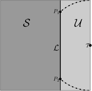
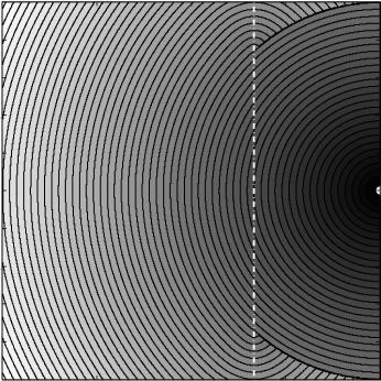
Refer to caption
Refer to caption
Figure 6. Left: an illustration of the domain. The darker region is 𝒮𝒮\mathcal{S} and the lighter region is 𝒰𝒰\mathcal{U}. The target is 𝒯=(1,0)𝒯10\mathcal{T}=(1,0). The black dotted line is the circle of radius B=1𝐵1B=1 centered about 𝒯𝒯\mathcal{T} in 𝒰𝒰\mathcal{U}. Right: a contour plot of the numerical solution of w(x,y,1)𝑤𝑥𝑦1w(x,y,1) for grid size N=961𝑁961N=961. The vertical white dotted line is the interface between 𝒮𝒮\mathcal{S} and 𝒰𝒰\mathcal{U} at x=1/3𝑥13x=1/3.
N𝑁N h L1(Ωe)subscript𝐿1subscriptΩ𝑒L_{1}(\Omega_{e}) rate L(Ωeϵ)subscript𝐿superscriptsubscriptΩ𝑒italic-ϵL_{\infty}(\Omega_{e}^{\epsilon}), ϵ=3hitalic-ϵ3\epsilon=3h rate L(Ωeϵ)subscript𝐿superscriptsubscriptΩ𝑒italic-ϵL_{\infty}(\Omega_{e}^{\epsilon}), ϵ=0.1italic-ϵ0.1\epsilon=0.1 rate
61 1/30 0.0612 - 0.0681 - 0.0681 -
121 1/60 0.0309 0.99 0.0513 0.41 0.0416 0.71
241 1/120 0.0151 1.03 0.0401 0.36 0.0255 0.71
481 1/240 0.0076 0.99 0.0265 0.60 0.0151 0.76
961 1/480 0.0039 0.96 0.0162 0.71 0.0090 0.75
Table 6.1. Errors measured against the exact solution for various grid sizes N𝑁N.

6.2. Geometry of 𝒮𝒮\mathcal{S} and the number of iterations

We illustrate how the information propagates within the main loop of Algorithm 2. Since the reachable part of the safe set (𝒮subscript𝒮\mathcal{S}_{\mathcal{R}}) is obtained iteratively, it might seem natural to expect that the iterative process stops once all the reachable components of 𝒮𝒮\mathcal{S} are already found (i.e., once 𝒮k=𝒮superscriptsubscript𝒮𝑘subscript𝒮\mathcal{S}_{\mathcal{R}}^{k}=\mathcal{S}_{\mathcal{R}}, also ensuring that MFLk=MFL𝑀𝐹superscript𝐿𝑘𝑀𝐹𝐿MFL^{k}=MFL). Here we show that this generally need not be the case and the value function Wksuperscript𝑊𝑘W^{k} might require more iterations to converge after that point. Roughly speaking, this occurs when the order of traversal of some optimal path through a sequence of connected components of 𝒮subscript𝒮\mathcal{S}_{\mathcal{R}} differs from the order in which those components were discovered. Mathematically, the extra iterations are needed because the correct values of W2ksuperscriptsubscript𝑊2𝑘W_{2}^{k} are not yet known on ΓΓ\Gamma, and the values of W1k+1superscriptsubscript𝑊1𝑘1W_{1}^{k+1} on the MFL are still incorrect as a result.
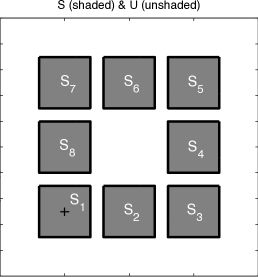
Refer to caption
Refer to caption
Figure 7. Left: The sets 𝒮𝒮\mathcal{S}, 𝒰𝒰\mathcal{U} and the target 𝒯=(0.5,0.5)𝒯0.50.5\mathcal{T}=(-0.5,-0.5) shown by a black cross. The eight connected components S1,S2,,S8subscript𝑆1subscript𝑆2subscript𝑆8S_{1},S_{2},\dots,S_{8} of 𝒮𝒮\mathcal{S} are labeled. Right: the speed function. Note the slow speed in the corridor C8subscript𝐶8C_{8} between the S1subscript𝑆1S_{1} and S8subscript𝑆8S_{8}.

Consider the following “pathological” example (shown in Figure 7): 𝒮𝒮\mathcal{S} consists of eight square blocks S1,S2,,S8subscript𝑆1subscript𝑆2subscript𝑆8S_{1},S_{2},\dots,S_{8} with side lengths 0.4, enumerated counter-clockwise, with 𝒯S1𝒯subscript𝑆1\mathcal{T}\in S_{1}. To simplify the discussion, we assume that S9:=S1assignsubscript𝑆9subscript𝑆1S_{9}:=S_{1} and introduce the notation for “unsafe corridors” between the safe squares:

Ci=convex_hull(SiSi+1)𝒰;i=1,,8.formulae-sequencesubscript𝐶𝑖convex_hullsubscript𝑆𝑖subscript𝑆𝑖1𝒰𝑖18C_{i}\;=\;\text{convex\_hull}(S_{i}\cup S_{i+1})\,\cap\,\mathcal{U};\qquad i=1,\ldots,8.

We set

f(𝒙)={10𝒙𝒮C1C2C7,0.1otherwise.𝑓𝒙cases10𝒙𝒮subscript𝐶1subscript𝐶2subscript𝐶70.1otherwise.f(\mbox{\boldmath${x}$})=\begin{cases}10&\mbox{\boldmath${x}$}\in\mathcal{S}\cup C_{1}\cup C_{2}\cup\cdots\cup C_{7},\\ 0.1&\text{otherwise.}\end{cases}

Note that f=0.1𝑓0.1f=0.1 in C8subscript𝐶8C_{8}. The target is 𝒯=(0.5,0.5)𝒯0.50.5\mathcal{T}=(-0.5,-0.5) and the maximum budget is B=1.5𝐵1.5B=1.5. Note that for all the starting positions in S2,,S8subscript𝑆2subscript𝑆8S_{2},\ldots,S_{8}, the corresponding constrained optimal trajectories will run toward S1subscript𝑆1S_{1} clockwise (to avoid crossing through the slow region in C8subscript𝐶8C_{8}). The same is true for all starting positions in C1,,C7subscript𝐶1subscript𝐶7C_{1},\ldots,C_{7} and even for points in C8subscript𝐶8C_{8} that are significantly closer to S8subscript𝑆8S_{8}.

This problem was specifically designed to illustrate the difference between the evolution of the reachable set Ωk=𝒰k𝒮ksuperscriptsubscriptΩ𝑘superscriptsubscript𝒰𝑘superscriptsubscript𝒮𝑘{\Omega}_{\mathcal{R}}^{k}={\mathcal{U}}_{\mathcal{R}}^{k}\cup\mathcal{S}_{\mathcal{R}}^{k} and the evolution of the “fully converged” set k={𝒙wk(𝒙)=w(𝒙)}superscript𝑘conditional-set𝒙superscript𝑤𝑘𝒙𝑤𝒙\mathcal{F}^{k}=\{\mbox{\boldmath${x}$}\mid w^{k}(\mbox{\boldmath${x}$})=w(\mbox{\boldmath${x}$})\}, on which the value function is correct after the k𝑘k-th iteration. Both sets eventually contain all Sisubscript𝑆𝑖S_{i}’s and Cisubscript𝐶𝑖C_{i}’s, but a careful examination of Figure 8 reveals the difference. For the reachable set, Ω1=S1superscriptsubscriptΩ1subscript𝑆1{\Omega}_{\mathcal{R}}^{1}=S_{1} initially, and the algorithm iteratively discovers the reachable Sisubscript𝑆𝑖S_{i}’s (and Cisubscript𝐶𝑖C_{i}’s) simultaneously in both the clockwise and counter-clockwise directions. More than one Sisubscript𝑆𝑖S_{i} can be “discovered” per iteration in each direction: e.g., at iteration k=3𝑘3k=3, Phase I of the algorithm discovers that C2C3𝒰3subscript𝐶2subscript𝐶3superscriptsubscript𝒰3C_{2}\cup C_{3}\subset{\mathcal{U}}_{\mathcal{R}}^{3} owing to a feasible path that “passes through the corner” shared by C2subscript𝐶2C_{2} and C3subscript𝐶3C_{3}; this subsequently leads to Phase II discovering that S3S4𝒮3subscript𝑆3subscript𝑆4superscriptsubscript𝒮3S_{3}\cup S_{4}\subset\mathcal{S}_{\mathcal{R}}^{3}. The same argument implies that C6C7𝒰3subscript𝐶6subscript𝐶7superscriptsubscript𝒰3C_{6}\cup C_{7}\subset{\mathcal{U}}_{\mathcal{R}}^{3} and S6S7𝒮3subscript𝑆6subscript𝑆7superscriptsubscript𝒮3S_{6}\cup S_{7}\subset\mathcal{S}_{\mathcal{R}}^{3}. After one more iteration we already see that S5𝒮4subscript𝑆5superscriptsubscript𝒮4S_{5}\subset\mathcal{S}_{\mathcal{R}}^{4} and another iteration is sufficient to recover the entire reachable set Ω=Ω5subscriptΩsuperscriptsubscriptΩ5{\Omega}_{\mathcal{R}}={\Omega}_{\mathcal{R}}^{5}.

However, on a large part of ΩsubscriptΩ{\Omega}_{\mathcal{R}} the value function is still quite far from correct at that point; e.g., a comparison of level curves in C5subscript𝐶5C_{5} and S5subscript𝑆5S_{5} shows that C55subscript𝐶5superscript5C_{5}\not\in\mathcal{F}^{5}. Since 𝒯S1𝒮𝒯subscript𝑆1𝒮\mathcal{T}\in S_{1}\subset\mathcal{S} and S1subscript𝑆1S_{1} is convex, we have S11subscript𝑆1superscript1S_{1}\subset\mathcal{F}^{1}. It is similarly easy to see that (k1Ck1Sk)ksuperscript𝑘1subscript𝐶𝑘1subscript𝑆𝑘superscript𝑘(\mathcal{F}^{k-1}\cup C_{k-1}\cup S_{k})\subset\mathcal{F}^{k} for k=2,,8𝑘28k=2,...,8. Thus, it takes eight iterations to correctly compute w𝑤w on the entire safe set and one more iteration to cover those unsafe points (including a part of C8subscript𝐶8C_{8}), whose optimal trajectories take them first to S8subscript𝑆8S_{8} and then clockwise (through the “fast belt”) toward S1subscript𝑆1S_{1}. We note that, as iterations progress, the value function need not be converged on recently discovered components of 𝒮subscript𝒮\mathcal{S}_{\mathcal{R}}, even if the level sets already show the generally correct (clockwise) direction of optimal trajectories. For example, it might seem that S86subscript𝑆8superscript6S_{8}\in\mathcal{F}^{6}, but a careful comparison of level curves shows that the value function is still incorrect even on C6subscript𝐶6C_{6} and S7subscript𝑆7S_{7}. (This is due to the fact that the reachability of S8subscript𝑆8S_{8} is discovered by feasible trajectories passing through a common corner of C6subscript𝐶6C_{6} and C7subscript𝐶7C_{7}.) Figure 9 confirms this by showing the \infty-norm of the value changes after each iteration. We observe two key events:
\bullet\; the initial drop in value changes, when ΩsubscriptΩ{\Omega}_{\mathcal{R}} is fully discovered after iteration five
(at which point the errors are still independent of hh and ΔbΔ𝑏\Delta b);
\bullet\; and the convergence (i.e., the drop of value changes to the machine precision) after iteration nine.
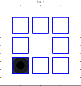
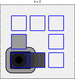
Refer to caption
Refer to caption
Refer to caption
Refer to caption
Refer to caption
Refer to caption
Figure 8. The first six iterations (each after Phase II) of Wksuperscript𝑊𝑘W^{k} on b=B𝑏𝐵b=B. The contour lines are scaled logarithmically to avoid bunching in the slow regions of 𝒰𝒰\mathcal{U}.
Refer to caption
Figure 9. The max-norm difference between consecutive W1ksuperscriptsubscript𝑊1𝑘W_{1}^{k} and W2ksuperscriptsubscript𝑊2𝑘W_{2}^{k}. The numerical convergence tolerance is shown by the thick horizontal dotted line. Both W10superscriptsubscript𝑊10W_{1}^{0} and W20superscriptsubscript𝑊20W_{2}^{0} were set to 103superscript10310^{3}.

6.3. Optimal paths and the effect of varying B𝐵B

We now consider two examples with inhomogeneous speed functions. The first scenario involves a discontinuous speed function that is slow in the safe set:

f(𝒙)={1𝒙𝒰0.3𝒙𝒮.𝑓𝒙cases1𝒙𝒰0.3𝒙𝒮f(\mbox{\boldmath${x}$})=\begin{cases}1&\mbox{\boldmath${x}$}\in\mathcal{U}\\ 0.3&\mbox{\boldmath${x}$}\in\mathcal{S}.\end{cases}

This example presents a curious dilemma: any good path will try to avoid 𝒮𝒮\mathcal{S} to travel faster to 𝒯𝒯\mathcal{T}, but it must visit 𝒮𝒮\mathcal{S} at least every B𝐵B distance to keep the budget from depleting. The numerical test for B=0.4𝐵0.4B=0.4 is shown in the center plot of Figure 10. The computed “optimal path” tends to travel along the interface ΓΓ\Gamma on the 𝒰𝒰\mathcal{U} side while occasionally making short visits into 𝒮𝒮\mathcal{S} to reset the budget444 Since Γ𝒮Γ𝒮\Gamma\subset\mathcal{S}, it is not really possible to quickly travel on the ΓΓ\Gamma itself. As a result, an optimal control does not exist, though the value function w1subscript𝑤1w_{1} is still well-defined. This lack of optimal control does not contradict the compatibility condition (29) (i.e., w1=w2subscript𝑤1subscript𝑤2w_{1}=w_{2} on ΓΓ\Gamma). The numerically recovered “optimal” trajectory shown in this Figure is actually “ε𝜀\varepsilon-suboptimal”, where ϵ0italic-ϵ0\epsilon\to 0 under the grid refinement. . We have added small white circles to the plot in Figure 10 (center) to identify the locations of these “reentry” points.

The second example illustrates the robustness of the numerical scheme to non-trivial speed functions in 𝒰𝒰\mathcal{U}: we set B=0.4𝐵0.4B=0.4 and

f(𝒙)=10.5sin(5πx)sin(5πy).𝑓𝒙10.55𝜋𝑥5𝜋𝑦f(\mbox{\boldmath${x}$})=1-0.5\sin(5\pi x)\sin(5\pi y).

The computed value function and a sample path are shown in the right plot of Figure 10.

Refer to caption
Refer to caption
Refer to caption
Figure 10. Sample optimal paths on the “islands” example with inhomogeneous speed functions.

Next, we give numerical examples showing the effects of varying B𝐵B. Figure 11 illustrates these effects on the “islands” examples (as in figure 10). The speeds were set to f=1𝑓1f=1 on all of the domain. While the optimal path is computed from the same initial point (0.8,0.5)0.80.5(0.8,0.5), note the large changes in its global behavior.
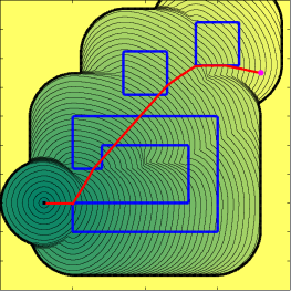
Refer to caption
Refer to caption
Refer to caption
Figure 11. Sample optimal paths on the “islands” example for varying B𝐵B. Left to right: B=0.3𝐵0.3B=0.3, 0.4 and 0.5, respectively.

6.4. Constrained contiguous visibility time.

We apply Algorithm 2 to a problem involving visibility exposure: suppose the objective is to move a robot towards a target in the shortest time, among opaque and impenetrable obstacles, while avoiding “prolonged exposure” to a static enemy observer. In our budget reset problem setting, we impose the prolonged exposure constraint by letting the enemy-visible region be 𝒰𝒰\mathcal{U} and the non-visible region as 𝒮𝒮\mathcal{S}. This is similar to the problem considered in [29], except that once the robot enters the non-visible region, it is again allowed to travel through the visible region up to the time B𝐵B.

The domain consists of four obstacles which act both as state constraints and as occluders. The static observer is placed at (0.8,0.8)0.80.8(0.8,0.8), and the corresponding visible set is computed by solving an auxiliary (static and linear) PDE on ΩΩ\Omega [39]. We compute the value function and optimal paths for the same starting location but two different exposure budgets: B=0.15𝐵0.15B=0.15 and B=0.3𝐵0.3B=0.3, see figure 12. Note that, for small B𝐵B, the budget is insufficient to directly travel across the 𝒰𝒰\mathcal{U} ‘corridor’ between the “shadows” of the larger foreground obstacles; for the larger B𝐵B this shortcut is feasible, thus reducing the path length.
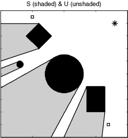
Refer to caption
Refer to caption
Refer to caption
Figure 12. The problem of constrained contiguous visibility time. The static observer location is shown by an asterisk. Left: the observer-viewable region is white; the occluders/obstacles are black, and their “shadows” are gray. The objective of is to find the quickest path connecting the two small squares while avoiding prolonged enemy-exposure. Center and right: contour plots of W𝑊W at b=B𝑏𝐵b=B and the constrained optimal paths with B=0.15𝐵0.15B=0.15 and 0.3, respectively.

7. Conclusions.

In this paper we focused on computational methods for optimal control of budget-constrained problems with resets. In the deterministic case on graphs, we explained how such problems can be solved by noniterative (label-setting) methods. We then introduced new fast iterative methods, suitable for both deterministic and stochastic problems on graphs, as well as for continuous deterministic budget reset problems. Throughout, we utilized the causal properties of the value function to make sure that dynamic programming equations are solved efficiently on the new extended domain. In the appendix we also describe an iterative algorithm on the original (non-extended) domain for solving a related simpler problem of finding the budget-reset-“reachable” parts of the state space.

We presented empirical evidence of convergence and illustrated other properties of our methods on several examples, including path-planning under constraints on “prolonged exposure” to an enemy observer. Even though all selected examples are isotropic in cost and dynamics, only minor modifications (with no performance penalties) are needed to treat anisotropy in secondary cost K^^𝐾\hat{K}. Anisotropies in primary cost and/or dynamics can also be easily treated by switching to a different (non-iterative or fast iterative) method on the safe set 𝒮𝒮\mathcal{S}. Several other natural extensions are likely to be more computationally expensive, but can be handled in the same framework:

  • In some applications the resource restoration is more realistically modeled not as an instantaneous reset, but as a continuous process on 𝒮𝒮\mathcal{S}. Alternatively, resets might be also modeled as conscious/optional control decisions available on 𝒮𝒮\mathcal{S}, with an instantaneous penalty in primary cost.

  • Differential games can be similarly modified to account for limited (and possibly renewable) resource budgets.

  • More generally, both the dynamics and the budget changes might be affected by some random events, leading to stochastic trajectories in the extended domain.

  • It would be interesting to extend the method to problems with constraints on multiple reset-renewable resources.

For problems with a fixed starting position, significant computational savings could be attained by adopting A*-type domain restriction algorithms [16]. All of these extensions are of obvious practical importance in realistic applications, and we hope to address them in the future. Finally, more work is clearly needed to provide proofs of convergence of semi-Lagrangian schemes to discontinuous viscosity solutions of hybrid systems.

Appendix A Determining the Reachable Set without expanding the state space.

For certain applications, one may be interested in computing only the reachable sets:

Ω={(𝒙,b)w(𝒙,b)<}Ω¯.subscriptΩconditional-set𝒙𝑏𝑤𝒙𝑏¯Ω{\Omega}_{\mathcal{R}}=\{(\mbox{\boldmath${x}$},b)\mid w(\mbox{\boldmath${x}$},b)<\infty\}\subset\bar{\Omega}.

While ΩsubscriptΩ{\Omega}_{\mathcal{R}} is indeed a byproduct of Algorithm 2, the goal of this section is to recover ΩsubscriptΩ{\Omega}_{\mathcal{R}} by a “lower dimensional” algorithm; e.g., using only computations on a grid 𝒢𝒢\mathcal{G} in Ω¯𝑹n¯Ωsuperscript𝑹𝑛\overline{\Omega}\subset\mbox{\boldmath${R}$}^{n}.

We note that the reachable set can be alternatively defined as Ω={(𝒙,b)v(𝒙)b}subscriptΩconditional-set𝒙𝑏𝑣𝒙𝑏{\Omega}_{\mathcal{R}}=\{(\mbox{\boldmath${x}$},b)\mid v(\mbox{\boldmath${x}$})\leq b\}, where v(𝒙)𝑣𝒙v(\mbox{\boldmath${x}$}) is the minimum needed starting budget, defined in (42) and (43). Thus, it suffices to compute v𝑣v from (44), which in turn requires knowing 𝒮={𝒙𝒮w2(𝒙)<}subscript𝒮conditional-set𝒙𝒮subscript𝑤2𝒙\mathcal{S}_{\mathcal{R}}=\{\mbox{\boldmath${x}$}\in\mathcal{S}\mid w_{2}(\mbox{\boldmath${x}$})<\infty\} to impose the boundary condition (43). We take an approach similar to Algorithm 2, by iteratively growing the known reachable set. The main difference is, instead of computing w1ksuperscriptsubscript𝑤1𝑘w_{1}^{k} on Ω𝒰subscriptΩ𝒰\Omega_{\mathcal{U}}, we solve a simpler boundary value problem on 𝒰𝒰\mathcal{U} itself – here we only need to know whether 𝒯={𝒙Ωq(𝒙)<}𝒯conditional-set𝒙Ω𝑞𝒙\mathcal{T}=\{\mbox{\boldmath${x}$}\in\partial\Omega\mid q(\mbox{\boldmath${x}$})<\infty\} is reachable (from each point in 𝒰𝒰\mathcal{U} and starting with a given budget), instead of finding the minimum cost of reaching it.

To this end, we introduce the auxiliary functions gk:Ω𝑹:superscript𝑔𝑘Ω𝑹g^{k}\colon\Omega\rightarrow\mbox{\boldmath${R}$}, computed iteratively in tandem with vksuperscript𝑣𝑘v^{k}, that can be used to extract the reachable sets in the safe set: 𝒮k={𝒙𝒮gk(𝒙)<}superscriptsubscript𝒮𝑘conditional-set𝒙𝒮superscript𝑔𝑘𝒙\mathcal{S}_{\mathcal{R}}^{k}=\{\mbox{\boldmath${x}$}\in\mathcal{S}\mid g^{k}(\mbox{\boldmath${x}$})<\infty\}. Similar to the recursive algorithm in section 5.2, we define initially

(53) v0(𝒙)=g0(𝒙)={0𝒙𝒯,otherwise;superscript𝑣0𝒙superscript𝑔0𝒙cases0𝒙𝒯otherwise\displaystyle v^{0}(\mbox{\boldmath${x}$})=g^{0}(\mbox{\boldmath${x}$})=\begin{cases}0&\mbox{\boldmath${x}$}\in\mathcal{T},\\ \infty&\text{otherwise};\end{cases}

the k𝑘k-th auxiliary function is defined as the (discontinuous) viscosity solution of the boundary value problem

(54) gk(𝒙)normsuperscript𝑔𝑘𝒙\displaystyle\|\nabla g^{k}(\mbox{\boldmath${x}$})\| =0𝒙int(𝒮),formulae-sequenceabsent0𝒙int𝒮\displaystyle=0\qquad\mbox{\boldmath${x}$}\in\text{int}(\mathcal{S}),
gk(𝒙)superscript𝑔𝑘𝒙\displaystyle g^{k}(\mbox{\boldmath${x}$}) ={0𝒙𝒯lim inf𝒙𝒙𝒙𝒰vk(𝒙)𝒙Γ\𝒯otherwise.absentcases0𝒙𝒯subscriptlimit-infimumFRACOPsuperscript𝒙𝒙superscript𝒙𝒰superscript𝑣𝑘𝒙𝒙\Γ𝒯otherwise\displaystyle=\begin{cases}0&\mbox{\boldmath${x}$}\in\mathcal{T}\\ \liminf\limits_{\mbox{\boldmath${x}$}^{\prime}\to\mbox{\boldmath${x}$}\atop\mbox{\boldmath${x}$}^{\prime}\in\mathcal{U}}v^{k}(\mbox{\boldmath${x}$})&\mbox{\boldmath${x}$}\in\Gamma\backslash\mathcal{T}\\ \infty&\text{otherwise}.\end{cases}

(See Remark 5.2 regarding the ‘liminf’ in the boundary condition above.) The MFLksuperscriptMFL𝑘\text{MFL}^{k} function vksuperscript𝑣𝑘v^{k} is defined as described in section 5.4 except that 𝒮k1superscriptsubscript𝒮𝑘1\mathcal{S}_{\mathcal{R}}^{k-1} is no longer computed using w1ksuperscriptsubscript𝑤1𝑘w_{1}^{k}; instead, it is computed from gk1superscript𝑔𝑘1g^{k-1} via the formula 𝒮k1={𝒙𝒮gk1(𝒙)<}superscriptsubscript𝒮𝑘1conditional-set𝒙𝒮superscript𝑔𝑘1𝒙\mathcal{S}_{\mathcal{R}}^{k-1}=\{\mbox{\boldmath${x}$}\in\mathcal{S}\mid g^{k-1}(\mbox{\boldmath${x}$})<\infty\}. Note that (54) implies that for each (closed) connected component 𝒮superscript𝒮\mathcal{S}^{\prime} of 𝒮𝒮\mathcal{S},

gk(𝒙)=min𝒙𝒮gk(𝒙), for all 𝒙𝒮,k=0,1,2formulae-sequencesuperscript𝑔𝑘𝒙subscriptsuperscript𝒙superscript𝒮superscript𝑔𝑘superscript𝒙formulae-sequence for all 𝒙superscript𝒮𝑘012g^{k}(\mbox{\boldmath${x}$})=\min_{\mbox{\boldmath${x}$}^{\prime}\in\partial\mathcal{S}^{\prime}}g^{k}(\mbox{\boldmath${x}$}^{\prime}),\quad\text{ for all }\mbox{\boldmath${x}$}\in\mathcal{S}^{\prime},k=0,1,2\dots

Once the iterative procedure reaches a steady state, the approximation to v𝑣v can be used to extract (an approximation to) the reachable set ΩsubscriptΩ\Omega_{\mathcal{R}}. An important observation is that 𝒮ksuperscriptsubscript𝒮𝑘\mathcal{S}_{\mathcal{R}}^{k} represents all point in 𝒮𝒮\mathcal{S} that can be reached from 𝒯𝒯\mathcal{T} by a feasible path containing at most k𝑘k contiguous segments through 𝒮\𝒯\𝒮𝒯\mathcal{S}\backslash\mathcal{T}. Thus, under the assumption that the number of connected components of 𝒮𝒮\mathcal{S} is finite, the algorithm will converge in a finite number steps.

The numerical approximations Vksuperscript𝑉𝑘V^{k}, Gksuperscript𝐺𝑘G^{k} of vksuperscript𝑣𝑘v^{k}, gksuperscript𝑔𝑘g^{k}, respectively, can be solved on 𝒢𝒢\mathcal{G} using standard numerical methods described in section 5.1. The iterative method is outlined in Algorithm 3.

1Initialization:
2 V0(𝒙)=G0(𝒙)={0𝒙𝒢,𝒙𝒢\𝒢;superscript𝑉0𝒙superscript𝐺0𝒙cases0for-all𝒙𝒢for-all𝒙\𝒢𝒢V^{0}(\mbox{\boldmath${x}$})=G^{0}(\mbox{\boldmath${x}$})=\begin{cases}0&\forall\mbox{\boldmath${x}$}\in\partial\mathcal{G},\\ \infty&\forall\mbox{\boldmath${x}$}\in\mathcal{G}\backslash\partial\mathcal{G};\\ \end{cases}
3
4Main Loop:
5 foreach k=1,2,𝑘12italic-…k=1,2,\dots until Vksuperscript𝑉𝑘V^{k} and Gksuperscript𝐺𝑘G^{k} stop changing do
6       Compute Vksuperscript𝑉𝑘V^{k}, using Gk1superscript𝐺𝑘1G^{k-1} to specify 𝒢𝒮k1𝒢superscriptsubscript𝒮𝑘1\mathcal{G}\cap\mathcal{S}_{\mathcal{R}}^{k-1};
7       Compute Gksuperscript𝐺𝑘G^{k} from equation 54, using Vksuperscript𝑉𝑘V^{k} on 𝒢𝒰subscript𝒢𝒰\mathcal{G}_{\mathcal{U}};
8      
9 end foreach
10
Algorithm 3 Reachability algorithm for the budget reset problem.

As an illustration, we implemented Algorithm 3 and applied it to the same problem as in the left plot of Figure 11 (case B=0.3𝐵0.3B=0.3). The first four iterations are shown in Figure 13. The domain [1,1]2superscript112[-1,1]^{2} was discretized on a 400×400400400400\times 400 grid. The algorithm halted after five iterations and took 0.45 seconds.
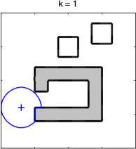
Refer to caption
Refer to caption
Refer to caption
Refer to caption
Figure 13. First four iterations for of Algorithm 3. The blue contours depict the level set {Vk(𝒙)=B=0.3}superscript𝑉𝑘𝒙𝐵0.3\{V^{k}(\mbox{\boldmath${x}$})=B=0.3\} and the shaded region is the set 𝒮k={Gk(𝒙)<}superscriptsubscript𝒮𝑘superscript𝐺𝑘𝒙\mathcal{S}_{\mathcal{R}}^{k}=\{G^{k}(\mbox{\boldmath${x}$})<\infty\} at the k𝑘k-th iteration. The target is shown by a ‘+’ at 𝒯=(0.7,0.4)𝒯0.70.4\mathcal{T}=(-0.7,-0.4).

Acknowledgments: The authors would like to thank Professor R. Tsai and Dr. Y. Landa, whose work on visibility and surveillance-evasion problems (joint with Ryo Takei) served as a starting point for this paper. The authors are grateful to them for helping to formulate the problem in section 6.4 and for many motivating discussions. The authors are also grateful to Ajeet Kumar, whose source code developed in [29] served as a starting point for our implementation described in section 4. RT would also like to thank Professors S. Osher and C. Tomlin for their encouragement and hospitality during the course of this work.

References

  • [1] Ahuja, R.K., Magnanti, T.L., & Orlin, J.B., Network Flows, Prentice Hall, Upper Saddle River, NJ, 1993.
  • [2] K. Alton & I. M. Mitchell, An Ordered Upwind Method with Precomputed Stencil and Monotone Node Acceptance for Solving Static Convex Hamilton-Jacobi Equations, J. of Scientific Computing, 51(2), pp. 313-348, 2012.
  • [3] M. Bardi & M. Falcone, An Approximation Scheme for the Minimum Time Function, SIAM J. Control Optim., 28, 950-965, 1990.
  • [4] M. Bardi & I. Capuzzo Dolcetta, Optimal Control and Viscosity Solutions of Hamilton-Jacobi-Bellman Equations, Birkhäuser Boston, 1997.
  • [5] M. Bardi, M. Falcone, & P. Soravia, Fully discrete schemes for the value function of pursuit-evasion games, “Advances in Dynamic Games and Applications”, T. Basar and A. Haurie (eds.), Birkhauser, (1994), 89-105.
  • [6] M Bardi, M Falcone, & P Soravia, Numerical methods for pursuit-evasion games via viscosity solutions in “Stochastic and Differential Games: Theory and Numerical Methods”, M. Bardi, T.E.S. Raghavan, and T. Parthasarathy (eds.), Birkhauser, (1999), 105-175.
  • [7] Bellman, R., On the Theory of Dynamic Programming, Proc. Nat. Acad. Sci., 38, pp. 716-719, 1952.
  • [8] Bertsekas, D.P., Network optimization: continuous & discrete models, Athena Scientific, Boston, MA, 1998.
  • [9] Bertsekas, D.P., Dynamic Programming and Optimal Control, 2nd Edition, Volumes I and II, Athena Scientific, Boston, MA, 2001.
  • [10] Bertsekas, D.P. & Tsitsiklis, J.N., An analysis of stochastic shortest path problems, Mathematics of Operations Research, 16(3), pp.580-595, 1991.
  • [11] Boué, M. & Dupuis, P., Markov chain approximations for deterministic control problems with affine dynamics and quadratic cost in the control, SIAM J. Numer. Anal., 36:3, pp.667-695, 1999.
  • [12] S. Cacace, E. Cristiani. M. Falcone, A local ordered upwind method for Hamilton-Jacobi and Isaacs equations, Proceedings of the 18th IFAC World Congress 2011.
  • [13] E. Carlini, M. Falcone, and R. Ferretti, A time adaptive semi Lagrangian approximation to Mean Curvature Motion, Num. Math. Advanced Applications- ENUMATH2005, Springer, Berlin (2006), pp. 732–739.
  • [14] E. Carlini, M. Falcone, N. Forcadel, and R. Monneau, Convergence of a Generalized Fast Marching Method with sign changing velocity for an eikonal equation, SIAM J. Numer. Anal. 46 (2008).
  • [15] A. Chacon, A. Vladimirsky, Fast two-scale methods for Eikonal equations, submitted to SIAM J. on Sci. Comp.
  • [16] Z. Clawson, A. Chacon, and A. Vladimirsky, Causal domain restriction for Eikonal equations, submitted to SIAM J. on Scientific Computing; preprint available from http://arxiv.org/abs/1309.2884
  • [17] Crandall, M.G. & Lions, P-L., Viscosity Solutions of Hamilton-Jacobi Equations, Tran. AMS, 277, pp. 1-43, 1983.
  • [18] E. Cristiani, M. Falcone, A Fast Marching Method for Pursuit-Evasion Games, published electronically in “Communications to SIMAI Congress”, SIMAI 2006 (Baia Samuele, Ragusa, Italy, May 22-26, 2006), Vol. 1, 2006.
  • [19] R. Dial, Algorithm 360: Shortest path forest with topological ordering, Comm. ACM, pp. 632–633, 1969.
  • [20] E.W. Dijkstra, A Note on Two Problems in Connection with Graphs, Numerische Mathematik, 1 (1959), pp. 269–271.
  • [21] M. Falcone, The Minimum Time Problem and Its Applications to Front Propagation, in “Motion by Mean Curvature and Related Topics”, Proceedings of the International Conference at Trento, 1992, Walter de Gruyter, New York, 1994.
  • [22] M. Falcone, A Numerical Approach to the Infinite Horizon Problem of Deterministic Control Theory, Applied Math. Optim., 15 (1987), pp. 1–13; corrigenda 23 (1991), pp. 213–214.
  • [23] M. Falcone & R. Ferretti, Discrete Time High-Order Schemes for Viscosity Solutions of Hamilton-Jacobi-Bellman Equations, Numerische Mathematik, 67 (1994), pp. 315–344.
  • [24] S. Fomel, S. Luo, and H. Zhao, Fast sweeping method for the factored eikonal equation, J. Comp. Phys. 228/17, pp. 6440-6455, 2009.
  • [25] Gonzales, R. & Rofman, E., On Deterministic Control Problems: an Approximate Procedure for the Optimal Cost, I, the Stationary Problem, SIAM J. Control Optim., 23, 2, pp. 242-266, 1985.
  • [26] Hansen, P., Bicriterion Path Problems, in Multiple Criteria Decision Making: Theory and Applications, G. Fandel and T. Gal (eds), Springer Verlag, Heidelberg, Germany, pp.109–127, 1980.
  • [27] Jaffe, J. M., Algorithms for finding paths with multiple constraints, Networks, 14, pp. 95–116, 1984.
  • [28] Kao, C.Y., Osher, S., & Qian, J., Lax-Friedrichs sweeping scheme for static Hamilton-Jacobi equations, J. Comput. Phys., 196:1, pp.367–391, 2004.
  • [29] A. Kumar and A. Vladimirsky, An efficient method for multiobjective optimal control and optimal control subject to integral constraints, Journal of Computational Mathematics, 28(4), pp.517–551, 2010.
  • [30] H.J. Kushner & P.G. Dupuis, Numerical Methods for Stochastic Control Problems in Continuous Time, Academic Press, New York, 1992.
  • [31] Martins, E.Q.V., On a Multicriteria Shortest Path Problem, European J. of Operational Research, Vol. 16, pp. 236–245, 1984.
  • [32] M. Motta and F. Rampazzo, Multivalued dynamics on a closed domain with absorbing boundary. Applications to optimal control problems with integral constraints, Nonlinear Analysis: Theory, Methods & Applications, vol. 41, no. 5–6, pp. 631–647, 2000.
  • [33] J.A. Sethian, A Fast Marching Level Set Method for Monotonically Advancing Fronts, Proc. Nat. Acad. Sci., 93, 4, pp. 1591–1595, February 1996.
  • [34] J.A. Sethian, Level Set Methods and Fast Marching Methods: Evolving Interfaces in Computational Geometry, Fluid Mechanics, Computer Vision and Materials Sciences, Cambridge University Press, 1996.
  • [35] Sethian, J.A., Fast Marching Methods, SIAM Review, Vol. 41, No. 2, pp. 199-235, 1999.
  • [36] J.A. Sethian & A. Vladimirsky, Ordered Upwind Methods for Static Hamilton-Jacobi Equations, Proc. Nat. Acad. Sci., 98, 20 (2001), pp. 11069–11074.
  • [37] J.A. Sethian & A. Vladimirsky, Ordered Upwind Methods for Static Hamilton-Jacobi Equations: Theory & Algorithms, SIAM J. on Numerical Analysis 41, 1 (2003), pp. 325-363.
  • [38] Soravia, P., Viscosity solutions and optimal control problems with integral constraints, Systems and Control Letters, 40 (2000), pp. 325–335.
  • [39] Tsai, Y.-H. R. and Cheng, L.-T. and Osher, S. and Burchard, P. and Sapiro, G. Visibility and its dynamics in a PDE based implicit framework, J. Comput. Phys. 199(1), 260–290, 2004.
  • [40] Tsai, Y.-H.R., Cheng, L.-T., Osher, S., & Zhao, H.-K., Fast sweeping algorithms for a class of Hamilton-Jacobi equations, SIAM J. Numer. Anal., 41:2, pp.659-672, 2003.
  • [41] J.N. Tsitsiklis, Efficient Algorithms for Globally Optimal Trajectories, IEEE Tran. Automatic Control, 40 (1995), pp. 1528–1538.
  • [42] A. Vladimirsky, Label-setting methods for Multimode Stochastic Shortest Path problems on graphs, Mathematics of Operations Research 33(4), pp. 821-838, 2008.
  • [43] D.J. White, Multi-objective infinite-horizon discounted Markov decision processes, J. of Mathematical Analysis and Applications, 89, pp. 639-647, 1982.
  • [44] Zhao, H.K., Fast Sweeping Method for Eikonal Equations, Math. Comp., 74, pp. 603-627, 2005.