Towards practical classical processing for the surface code

Abstract

The surface code is unarguably the leading quantum error correction code for 2-D nearest neighbor architectures, featuring a high threshold error rate of approximately 1%, low overhead implementations of the entire Clifford group, and flexible, arbitrarily long-range logical gates. These highly desirable features come at the cost of significant classical processing complexity. We show how to perform the processing associated with an $n\times n$ lattice of qubits, each being manipulated in a realistic, fault-tolerant manner, in $O(n^{2})$ average time per round of error correction. We also describe how to parallelize the algorithm to achieve $O(1)$ average processing per round, using only constant computing resources per unit area and local communication. Both of these complexities are optimal.

Quantum computing promises exponentially faster processing of certain problems, including factoring Shor (1994) and simulating quantum physics Lloyd (1996). Many quantum algorithms are now known Jordan (2012). The primary challenges are to mitigate and cope with the imperfections of quantum devices. The surface code Bravyi and Kitaev (1998); Dennis et al. (2002) supports a powerful quantum computing scheme Raussendorf and Harrington (2007); Raussendorf et al. (2007); Fowler et al. (2009) featuring an experimentally realistic threshold error rate of approximately 1% Wang et al. (2011) and requiring only a 2-D square lattice of qubits with nearest neighbor interactions. In this work, we describe how to perform the complex classical processing associated with the full, fault-tolerant scheme in a complexity-optimal manner. Using the current version of our code, we can simulate the fault-tolerant operation of millions of qubits, four orders of magnitude more than in any previous work. A detailed timing analysis can be found in Fowler et al. (2012).

Previous works on the classical processing of topological quantum error correction (QEC) have obtained results by making one of two significant modifications to the problem. Large lattice sizes have been simulated Duclos-Cianci and Poulin (2010), however only by assuming that 4-qubit operators can be measured perfectly. Small lattices have been simulated fault-tolerantly Raussendorf et al. (2007); Barrett and Stace (2010); Wang et al. (2010, 2011), however these works used the code of Kolmogorov Kolmogorov (2009) which does not support continuous processing of an arbitrary number of rounds of QEC. Our code now supports continuous fault-tolerant processing, using constant memory and with processing rate independent of the number of rounds.

The surface code involves a 2-D lattice of qubits with local stabilizers Bravyi and Kitaev (1998). We shall initially assume perfect stabilizer measurement to compare with Duclos-Cianci and Poulin (2010). Error chain endpoints anticommute with stabilizers leading to -1 stabilizer measurements. Each -1 is associated with a vertex. Assuming independent errors, long error chains are exponentially unlikely. Edges between vertices $v_{1}=(i_{1},j_{1})$, $v_{2}=(i_{2},j_{2})$ are given a weight $w_{12}$ to equal to their Manhattan separation $|i_{2}-i_{1}|+|j_{2}-j_{1}|$. Edges to boundaries are given a weight equal to their length.

We independently correct $X$ and $Z$ errors using the minimum weight perfect matching algorithm Edmonds (1965a, b). We use our own implementation which includes the concept of boundaries and returns edges such that every vertex is incident on exactly one edge and the total weight is minimal (Fig. 1). Corrections are applied along the chosen edges. Logical errors occur when after correction a chain of errors connecting opposing boundaries remains. Provided error chains are well separated, this is unlikely.

Figure 1: a) Example of a weighted graph with edges connecting vertices to labeled boundaries $b_{i}$. b) Set of edges such that every vertex is incident on exactly one edge and the total weight of all edges is minimal.

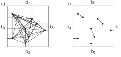
Clearly, a complete graph cannot be used if an $O(n^{2})$ runtime is to be achieved as a complete graph has $O(n^{4})$ edges. Simply generating a complete graph would therefore take a minimum of $O(n^{4})$ time. Progress can be made by noting that we are initially only considering data qubit errors and that a chain of errors between two -1 stabilizer measurements has length given by the Manhattan metric. If we choose a vertex and imagine looking at the graph from that vertex, nearby vertices casts shadows, where we define a point in the plane to be in shadow if it can be reached by a minimum length path passing through another vertex (Fig. 2a). We define a vertex to be shadowed if it is in shadow yet neighbors an unshadowed point, and deeply shadowed if all neighboring points are shadowed. Empirically, we find that if two vertices are deeply shadowed when viewed from one another, there always exists a minimum weight perfect matching that does not use an edge between them (Figs. 2b–c). This implies that such edges do not need to be included in the graph that describes the problem. This cuts the number of edges down to $O(n^{2})$. The validity of this approach has been verified with millions of simulations finding identical weight matchings with both the complete and shadowed approaches.

Figure 2: a) Plane as seen from vertex $v$. Vertices 1 and 2 are unshadowed, vertex 3 is shadowed, vertex 4 is deeply shadowed. b) A matching with an edge to a deeply shadowed vertex. c) An equal weight rearrangement of the matching. A lower weight matching is possible.

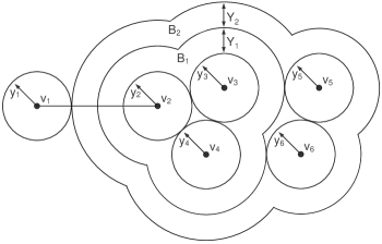
We now describe the minimum weight perfect matching algorithm, focusing on what is actually done. The original papers of Edmonds Edmonds (1965a, b) beautifully prove that the method works. First, some definitions. Let $G$ be a graph with vertices $\{v_{i}\}$, edges $\{e_{ij}\}$, and edge weights $\{w_{ij}\}$. Associate with each vertex $v_{i}$ a variable $y_{i}$, which can be thought of as the radius of a ball centered at $v_{i}$. Odd sets of vertices can also be made into blossoms $B_{k}$ that have their own variables $Y_{k}$, which can be thought of as the width of shell around every object in $B_{k}$. If a pair of blossoms intersect, then one is contained in the other. Define an edge $e_{ij}$ to be tight if $w_{ij}-y_{i}-y_{j}-\sum Y_{k}=0$, where the sum is over $k$ such that exclusively $v_{i}$ or $v_{j}$ is in $B_{k}$. This condition is pictorially depicted in Fig. 3.

Figure 3: An example of a tight edge. Edge $e_{12}$ has the property that $w_{12}-y_{1}-y_{2}-Y_{1}-Y_{2}=0$.

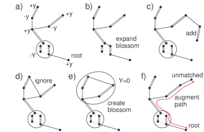
Define a node to be a vertex or blossom. Define a blossom to be unmatched if it contains an unmatched vertex. An alternating tree is a tree of nodes rooted on an unmatched node such that every path from the root to a leaf consists of alternating unmatched and matched edges. Alternating trees can only branch from the root and every second node from the root. Define branching nodes to be outer. Define all other nodes in the alternating tree to be inner. Fig. 4 shows all necessary alternating tree manipulations.

Figure 4: All required alternating tree manipulations. a) Increase outer node and decrease inner node $y$ values (or $Y$ if the node is a blossom), maintaining the tightness of all tree edges and potentially creating new tight edges connected to at least one outer node. b) Inner blossoms with $Y=0$ can be expanded into multiple inner and outer nodes and potentially some nodes that are no longer part of the tree. c) Outer–matched tight edges can be used to grow the alternating tree. d) Outer–inner tight edges can be ignored. e) Outer–outer tight edges make cycles that can be used to make blossoms. f) When another unmatched vertex $v$ is found, or an edge to a boundary $b$, the path from the unmatched vertex within the root node through the alternating tree to $v$ or $b$ is augmented, meaning matched edges become unmatched and unmatched edges become matched. This strictly increases the total number of vertices.

Given a weighted graph $G$, the following algorithm finds a minimum weight perfect matching.

1. If there are no unmatched vertices, return the list of matched edges.

2. Choose an unmatched vertex $v$ to be the root of alternating tree.

3. If no edges emanating from the outer nodes of the alternating tree are tight, henceforth called $O$-tight edges, increase the value of $y$ or $Y$ associated with each outer node while simultaneously decreasing the value of $y$ or $Y$ associated with each inner node until an edge becomes $O$-tight, or an inner blossom node $Y$ variable becomes 0 (Fig. 4a).

4. If an inner blossom node $Y$ variable becomes 0 and there are still no $O$-tight edges, expand that blossom and return to 3 (Fig. 4b).

5. Choose an $O$-tight edge $e$.

6. If $e$ leads to a matched node not already in the alternating tree, add the relevant unmatched and matched edge and associated nodes to the alternating tree and return to 3 (Fig. 4c).

7. If $e$ leads to an inner node, mark $e$ so it is not considered again during the growth of this alternating tree and return to 3 (Fig. 4d).

8. If $e$ leads to an outer node, add the unmatched edge to the alternating tree. There will now be a cycle of odd length. Collapse this cycle into a new blossom and associate a new variable $Y=0$ (Fig. 4e). Return to 3.

9. If $e$ leads to an unmatched vertex or boundary, add $e$ to the alternating tree and augment the path (unmatched$\leftrightarrow$matched) from the unmatched vertex within the root node to the end of $e$ (Fig. 4f). Destroy the alternating tree, keeping any newly formed blossoms. Return to 1.

On average, the algorithm only needs to consider a small local region around each vertex to find another unmatched vertex to pair with. This is a property of the graphs associated with topological QEC only, as the probability of needing to consider an edge of length $l$ decreases exponentially with $l$. This ensures that the runtime is $O(n^{2})$.

If we consider a standard square surface code with smooth boundaries top and bottom and rough boundaries left and right Fowler et al. (2009), we can randomly apply bit-flips $X$ with probability $p$ to the data qubits, perfectly measure the $Z$-stabilizers, construct a shadowed graph as described above, perform minimum weight perfect matching, apply corrections along the matched edges, and test for logical failure by checking whether there are an odd or even number of bit-flips along the top boundary. After correction, there can only be an odd number of bit-flips along the top boundary if a chain of bit-flips has formed from top to bottom boundary, indicating a logical error. The shortest topologically nontrivial chain is the distance $d$ of the code ($n=2d-1$). By performing many simulations, the probability of logical $X$ error $p_{L}$ versus $p$ can be plotted for a variety of distances (Fig. 5).

Figure 5: Logical $X$ error rate $p_{L}$ versus data qubit bit-flip probability $p$ for various code distances $d$ assuming perfect stabilizer measurement. The threshold error rate is 10.25%.

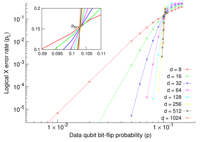
We observe a threshold error rate of 10.25%, versus 8.2% in the work of Duclos-Cianci and Poulin (2010), only slightly below the known ideal threshold error rate of 10.9% obtained using computationally inefficient techniques Ohzeki (2009); de Queiroz (2009). Furthermore, by comparing the fraction of the threshold error rate at which our curves cut a logical error rate of $4\times 10^{-3}$ to the equivalent quantities in Duclos-Cianci and Poulin (2010), it can be seen that our approach corrects twice as many errors at a given code distance, leading to a quadratic improvement of the logical error rate. Finally, the raw speed of our code is evident in our ability obtain data far below threshold.

High performance when assuming perfect stabilizer measurements enables comparison with existing results, however this case is not particularly interesting in practice. Only a fully fault-tolerant approach can be considered practical. When using fault-tolerant circuits to measure stabilizers and applying depolarizing noise, the simple 2-D square lattice with Manhattan metric considered above becomes a complicated 3-D lattice Wang et al. (2011) that has both spatial boundaries and a temporal boundary representing the latest round of stabilizer measurements. A number of modifications to the algorithm are required to account for these differences.

Firstly, calculating the complete shadow of a vertex does not work very well in the 3-D lattice. There are 12 outward directions to consider instead of 4 Wang et al. (2011), and the probability that all 12 directions are blocked by nearby vertices is low. Instead of exploring the entire unshadowed region, which can be exceedingly large, one needs to set a maximum radius of initial exploration. With high probability, only this initial region is required. Regions further from the vertex are only explored as required (if another unmatched vertex or boundary is not found in the initial region). The probability of requiring a region of radius $r$ decreases exponentially with $r$. In practice, we choose $r$ just large enough to ensure nearest and next nearest neighbor lattice locations are explored initially.

Secondly, the mobile temporal boundary introduces additional complexity. One must add new vertices to the problem as new data is obtained. This is straightforward, essentially just increasing the list of unmatched vertices. However, when growing an alternating tree, it is possible for the tree to attempt to grow into the future. We chose to solve this problem by undoing the growth of the tree and all of the changes its growth introduced — essentially running the algorithm backwards. Growth is only reattempted when data from more rounds of error correction is available.

Thirdly, detecting logical errors is more complex. One needs turn off errors, perform a perfect round of stabilizer measurement, match all vertices, apply corrections, detect logical errors as before by considering the top boundary, and then undo everything to return the simulator to its state before logical error detection. Note that this would not be done in a real computer. This procedure consumes negligible additional memory as a do/undo approach is used, and takes approximately 10 times as long as a single round of standard error correction.

Fourthly, it is nontrivial to ensure the amount of memory used remains finite as the simulation proceeds. With vanishingly small probability, in principle the entire history of stabilizer measurements is required to correctly match current time data. In practice, we keep track of the maximum distance in the past the algorithm has traversed to perform any matching, and store a fixed multiple of this distance, discarding any older data. Close to the threshold error rate, and especially above threshold, extremely large blossoms are created, involving thousands of vertices and hundreds of blossom layers. Storing these blossoms dominates the memory cost. The growth of large blossoms, which is a gradual process, provides a warning that more data needs to be stored, ensuring reliable processing.

With these modifications in mind, fault-tolerant simulation data is shown in Fig. 6. All data points represent one or more simulation instances run continuously until a total of 10,000 logical errors were observed, enabling reliable determination of the probability of logical error per round of error correction. Note that the threshold error rate is 0.9%, in contrast to prior work that estimated it at 1.1% Wang et al. (2011). This highlights the danger of estimating thresholds from small distance data only. The new code exactly reproduces the curves of the old code up to $d=13$, however the true threshold error rate is really only visible for $d>21$, distances at which the old code can not be run. This lowered threshold can be attributed to boundary effects, since boundary stabilizers are lower weight and hence more reliable. The physical error rates at which a factor of 2 (10) improvement in logical error rate is observed when the code distance is increased by 2 remain 0.5% (0.2%) respectively, so this threshold error rate change is of no practical significance.

Figure 6: Logical $X$ error rate per round of error correction $p_{L}$ versus depolarizing probability $p$ for various code distances $d$ using fault-tolerant stabilizer measurement. The threshold error rate is 0.9%.

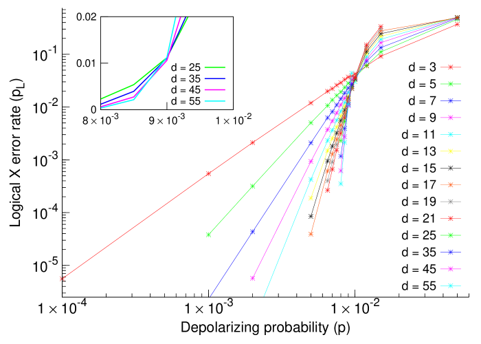
Memory limitations prevented the gathering of statistics near the threshold error rate at higher distances, however at $p=10^{-3}$ the vast blossoms that make high error rate correction so difficult do not occur, and it is straightforward to simulate distances as high as $d=1000$ — over 4 million qubits. Needless to say, no logical errors are observed in such a simulation. Each round of error correction takes under 3 seconds using a single core of an AMD Opteron, with each individual matching taking tens of microseconds. Given the algorithm uses only local information, it is in principle straightforward to parallelize, using a 2-D array of processors with each processor handling a fixed size patch of code. Inserting a small pause after each patch correction enables any patch with a randomly harder matching to catch up after lagging behind. This would enable the classical processing of an infinite lattice in constant average time per round of error correction, with the average time approaching the time for a single matching in the limit of low $p$ and high classical computing resources.

In summary, we have introduced an algorithm that finds a minimum weight perfect matching in $O(n^{2})$ time given a graph generated by an $n\times n$ lattice of qubits running the surface code fault-tolerantly. This algorithm parallelizes to $O(1)$ on an infinite lattice with constant computing resources per unit area. It is conceivable that a parallel implementation could achieve hundred microsecond processing of a round of error correction, sufficient to keep pace with ion trap quantum gates Hanneke et al. (2009). Additional ideas, including implementation in hardware, would be required to achieve the submicrosecond processing times required to keep pace with faster gates such as those found in superconducting circuits Mariantoni et al. (2011).

We acknowledge support from the Australian Research Council Centre of Excellence for Quantum Computation and Communication Technology (Project number CE110001027), and the US National Security Agency (NSA) and the Army Research Office (ARO) under contract number W911NF-08-1-0527.

References

- Shor (1994) P. W. Shor, in Proc. 35th Annual Symposium on Foundations of Computer Science (1994), pp. 124–134, quant-ph/9508027.
- Lloyd (1996) S. Lloyd, Science 273, 1073 (1996).
- Jordan (2012) S. Jordan, Quantum algorithm zoo, http://math.nist.gov/quantum/zoo/ (2012).
- Bravyi and Kitaev (1998) S. B. Bravyi and A. Y. Kitaev, quant-ph/9811052 (1998).
- Dennis et al. (2002) E. Dennis, A. Kitaev, A. Landahl, and J. Preskill, J. Math. Phys. 43, 4452 (2002), quant-ph/0110143.
- Raussendorf and Harrington (2007) R. Raussendorf and J. Harrington, Phys. Rev. Lett. 98, 190504 (2007), quant-ph/0610082.
- Raussendorf et al. (2007) R. Raussendorf, J. Harrington, and K. Goyal, New J. Phys. 9, 199 (2007), quant-ph/0703143.
- Fowler et al. (2009) A. G. Fowler, A. M. Stephens, and P. Groszkowski, Phys. Rev. A 80, 052312 (2009), arXiv:0803.0272.
- Wang et al. (2011) D. S. Wang, A. G. Fowler, and L. C. L. Hollenberg, Phys. Rev. A 83, 020302(R) (2011), arXiv:1009.3686.
- Fowler et al. (2012) A. G. Fowler, A. C. Whiteside, and L. C. L. Hollenberg, arXiv:1202.5602 (2012).
- Duclos-Cianci and Poulin (2010) G. Duclos-Cianci and D. Poulin, Phys. Rev. Lett. 104, 050504 (2010), arXiv:0911.0581.
- Barrett and Stace (2010) S. D. Barrett and T. M. Stace, Phys. Rev. Lett. 105, 200502 (2010), arXiv:1005.2456.
- Wang et al. (2010) D. S. Wang, A. G. Fowler, A. M. Stephens, and L. C. L. Hollenberg, Quant. Info. Comp. 10, 456 (2010), arXiv:0905.0531.
- Kolmogorov (2009) V. Kolmogorov, Math. Prog. Comp. 1, 43 (2009).
- Edmonds (1965a) J. Edmonds, Canad. J. Math. 17, 449 (1965a).
- Edmonds (1965b) J. Edmonds, J. Res. Nat. Bur. Standards 69B, 125 (1965b).
- Ohzeki (2009) M. Ohzeki, Phys. Rev. E 79, 021129 (2009), arXiv:0811.0464.
- de Queiroz (2009) S. L. A. de Queiroz, Phys. Rev. B 79, 174408 (2009), arXiv:0902.4153.
- Hanneke et al. (2009) D. Hanneke, J. P. Home, J. D. Jost, J. M. Amini, D. Leibfried, and D. J. Wineland, Nature Physics 6, 13 (2009), arXiv:0908.3031.
- Mariantoni et al. (2011) M. Mariantoni, H. Wang, T. Yamamoto, M. Neeley, R. C. Bialczak, Y. Chen, M. Lenander, E. Lucero, A. D. O Connell, D. Sank, et al., arXiv:1109.3743 (2011).