Classification of Stellar Spectra with LLE

Abstract

We investigate the use of dimensionality reduction techniques for the classification of stellar spectra selected from the SDSS. Using local linear embedding (LLE), a technique that preserves the local (and possibly non-linear) structure within high dimensional data sets, we show that the majority of stellar spectra can be represented as a one dimensional sequence within a three dimensional space. The position along this sequence is highly correlated with spectral temperature. Deviations from this “stellar locus” are indicative of spectra with strong emission lines (including misclassified galaxies) or broad absorption lines (e.g. Carbon stars). Based on this analysis, we propose a hierarchical classification scheme using LLE that progressively identifies and classifies stellar spectra in a manner that requires no feature extraction and that can reproduce the classic MK classifications to an accuracy of one type.

I Introduction

Automatic classification of stellar data is a problem as old as the use of computers in astronomy. Since survey projects have begun presenting us with spectral data from literally hundreds of thousands of sources, it has become untenable to classify all of them “by hand.” Computer science provides several tools and algorithms available to help us alleviate the human experts’ work load. Neural networks Storrie-Lombardi et al. (1994); Singh et al. (1998) and Principal Component Analysis (PCA; Deeming 1964) are among the most popular computational tools presently used to tackle large sets of astronomical data. In this paper, we will consider a relatively new method: Local Linear Embedding (LLE) Roweis and Saul (2000).

At the heart of automated stellar classification is dimensionality reduction: taking a large number $N$ of $D\gg 1$ dimensional data (in this paper we consider $N=49,529$ stellar spectra sampled over $D=500$ wavelength bins), and projecting the data onto a basis such that the first $d\ll D$ dimensions contain the bulk of the physical information encoded in the data. LLE attempts to reduce the dimensionality of the input data points while preserving the non-linear relationships between them. It does so by analyzing the data incrementally, in small neighborhoods, rather than all at once. This is particularly useful for astronomical classification, as we shall see below, since it can be simultaneously sensitive to continuum and line shapes. Thus, LLE ought to provide a more robust object classification from fewer projected dimensions than PCA. Vanderplas and Connolly (2009) explored LLE as a means of characterizing the spectral energy distributions of galaxies. They found the method very effective and, in some cases, more accurate than traditional tests at distinguishing different types of galaxies (broad- and narrow-line QSO’s, emission line galaxies, quiescent galaxies, and absorption galaxies; see their Figure 2) without the need to identify and measure individual features in the galaxies’ spectra. We use their code to analyze 49,529 stellar spectra from the SDSS Data Release 7 (DR7) Abazajian et al. (2009). We specifically consider the ability of LLE to identify different types of objects (galaxies, stars, and QSOs). In the case of stars, we consider the ability of LLE to classify objects according to their MK spectral types. In Section II we will discuss past work on automated stellar classification using Principal Component Analyis (PCA). In Section III we will review the algorithm of LLE and contrast it with that of PCA. In Section IV we will present the results of spectral classification using only LLE analysis. In Section V we will contrast our results with those from PCA.

II Past Work with Principal Component Analysis

Most of the work to date has focused on Principal Component Analysis (PCA). PCA takes the data vectors and projects them onto an orthogonal basis made up of the eigenvectors of the correlation matrix of the unprocessed data. Theoretically, the originally high-dimensional data can be well-characterized by linear combinations of the few eigenvectors with the highest eigenvalues Bailer-Jones et al. (1998); McGurk et al. (2010). The use of PCA in analyzing large volumes of stellar data was first proposed by Deeming (1964). Deeming considered data from measurements of five spectral lines from G and K giants, projected them using PCA, and found that the component of each vector in the first projected coordinate was sufficient to characterize the corresponding star’s MK spectral type. This is obviously an oversimplified case since it deals with a data set comprised entirely of late-type stars. Figure 4 of Singh (2001) shows that adding early-type stars to the data set necessitates the addition of at least one extra PCA dimension to recreate Deeming’s successful classification.

Following Deeming, much of the work in PCA and stellar classification focused on using PCA to pre-process the data fed into artificial neural networks. Storrie-Lombardi et al. (1994) found that data must be projected onto a minimum of three eigencomponents in order to improve the MK classification performance of raw-data neural networks. Singh et al. (1998) found that at least 10 components were necessary to accurately reproduce classifications performed by human experts, but that use of between two and five eigencomponents reproduced human results to within three spectral subtypes (see their Table 2). This is the predominant theme of stellar classification with PCA projection: at least two eigencomponents are needed to reproduce the results of human experts Christian (1982); Whitney 1983a ; Beauchemin et al. (1991); Singh et al. (2001). We hope to show that LLE can improve on this performance by producing a single parameter that uniquely correlated with spectral type.

In addition to reproducing the MK classification of stellar spectra, there has been significant interest in using PCA to extract the physical properties (effective temperature, metallicity, gravity, etc.) of stars Whitney 1983b ; McGurk et al. (2010). Using stellar spectra from the SDSS DR7 Abazajian et al. (2009), McGurk et al. (2010) found a correlation between a star’s PCA decomposition and its metallicity. We will also consider the ability of LLE to extract physical information from stellar spectra.

Recently, PCA has also been applied to classifying the spectral energy distribution of galaxies Connolly et al. (1995); Bailer-Jones et al. (1998); Ronen et al. (1999); Yip et al. 2004a , and quasars Yip et al. 2004b . Cabanac et al. (2002) found that PCA can be effective at separating out stellar, galactic, and QSO spectra while simultaneously dividing the stellar spectra into spectral classes. Because our initial filtering of the data does not successfully remove all non-stellar spectra from our data set, we are able to test the ability of LLE to separate galactic from stellar sources as well.

III The LLE Algorithm

One shortcoming of PCA (already identified by Deeming in 1964) is that it relies on the assumption that all of the data considered can be well-described as a linear combination of all of the other data. If the data instead conforms to some underlying non-linear manifold (for example, if not only the presence but the intensity of lines varies between spectra; Connolly et al. 1995), PCA will wash that information out. LLE avoids such oversimplification by attempting to reconstruct each data point from a linear combination of only its $k$ nearest neighbors, where $k\ll N$. This local reconstruction is characterized in terms of a global weight matrix ${\bf W}$, i.e. the $i$th datapoint $\vec{x}^{i}$ is reconstructed as

$$\vec{x}^{i}=\sum_{j}^{N}{\bf W}_{ij}\vec{x}^{j}$$ (1)

where ${\bf W}_{ij}=0$ if the $j\text{th}$ data point is not one of $\vec{x}^{i}$’s $k$ nearest neighbors. Solving for ${\bf W}_{ij}$ is later referred to as the “training phase.” LLE projects the data down to a $d\ll D$-dimensional space by finding $d$-dimensional data points $\vec{y}$ such that the relationship (1) remains true, i.e.,

$$\vec{y}^{i}=\sum_{j}^{N}{\bf W}_{ij}\vec{y}^{j}$$ (2)

for the same weight matrix as above. The relationships between data points and their nearest neighbors remain linear, but the non-linear relationships between disparate neighborhoods are preserved. This final projection is an eigenvalue problem such that the $d$ projected dimensions correspond to the eigenvectors of the matrix

$${\bf M}=({\bf I}-{\bf W})({\bf I}-{\bf W})^{T}$$ (3)

with the smallest eigenvalues. For a more detailed description see Roweis and Saul (2000), de Ridder and Duin (2002) and Vanderplas and Connolly (2009).

Figure 1: A demonstration of the advantage of LLE over PCA. Figure 1 shows the unprocessed, three-dimensional input data. Figure 1 shows the result of a simple, two-dimensional PCA projection of the data. Figure 1 shows the result of a two-dimensional LLE projection of the data. Color-coding is consistent between samples. Note that the PCA projection confuses the relationship between points where curvature in Figure 1 is strongest. LLE correctly maps the data to its underlying manifold.

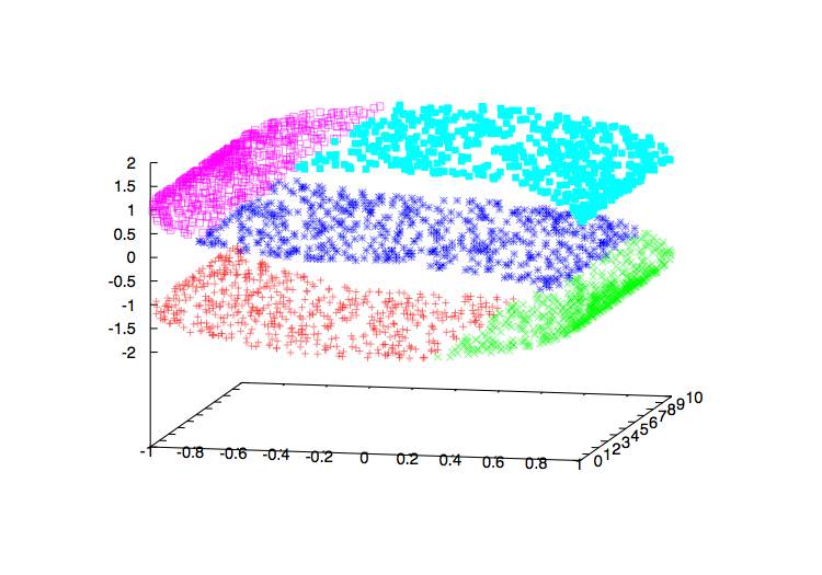
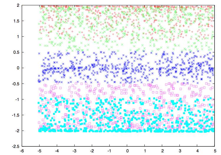
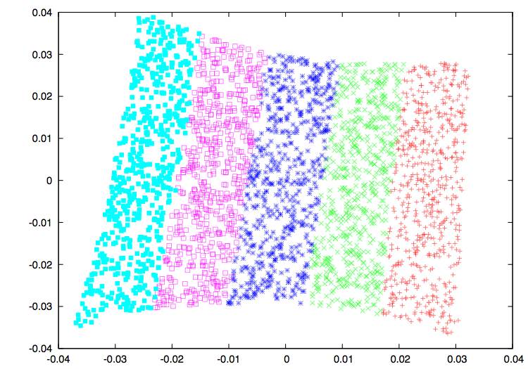
Figure 1 demonstrates the advantage of this neighborhood-by-neighborhood treatment of the data. Figure 1 posits some three-dimensional data on an embedded two-dimensional manifold. Figure 1 attempts to unwind the manifold using a simple two-dimensional PCA projection as described in Section 3 of Xiong et al (2011). The color bands are correctly ordered, however, they blend together where the embedding goes non-linear (where the ‘S’ shape curves in Figure 1). Figure 1 attempts to unwind the manifold using LLE. There is no blending. Because it divides the data into small neighborhoods, LLE is always treating quasi-linear subsets of the entire manifold. Linear projection as in equation (1) remains valid and the correct relationship between datapoints is preserved. This will be especially useful in spectroscopy, where objects can be related by their continua, their emission and absorption features, or some non-trivial combination of the two.

One disadvantage of the LLE algorithm is that, unlike PCA, it does not produce basis vectors onto which future data points can be projected for decomposition. The weight matrix in equation (1) means that the projection is dependent upon and unique to the points being projected. To add new points to a data set, one must redo the entire analysis from scratch. Conversely, in PCA, one simply decomposes the new points into the basis vectors already solved for. There are ways to modify the algorithm to avoid this complication. In their section 5.3, Vanderplas and Connolly (2009) propose a method in which, for each of the $N$ data points, the neighbors used to construct the weight matrix are chosen from only a subset of the data. This subset is selected to maximize the represented signal variance relative to the full data set. When new data points are added under this modification, one only needs to perform the nearest-neighbor search for the new points (as opposed to the full data set in the context of the new points) and re-run the algorithm from there. We adopt this modification in the work below, training our LLE projection on only 5,000 of the full 49,529 spectra in the data set.

Because LLE attempts to subdivide the original, non-linearly related data set into smaller, linearly-related data sets, it may not be applicable to data sparsely sample the non-linear space. It may be possible to address this concern by reducing the number of nearest neighbors used in constructing the weight matrix 1. It would probably be safer to avoid using LLE on small data sets.

IV Results

We use the same set of stellar spectra that Xiong et al. (2011) treat with PCA. Objects are chosen from the 85,564 DR7 sources classified as science-quality stellar spectra (though, as will be seen, further analysis reveals that some galactic spectra are included). Objects are rejected if they have redshift $z>0.36$, more than 20% of the pixels in the image are bad, their spectra contain large positive ($>10^{4}$) or negative ($<-100$) spikes in flux, their signal-to-noise ratio is less than 10, or their magnitude is less than 15.5. This results in 49,529 spectra to analyze. These spectra are reduced to 500 wavelength bins evenly spaced in $\log_{10}(\lambda)$. Gaps in the spectra due to bad pixels are filled in using the PCA eigenspectra of Xiong et al (2011). We transform the spectra to their rest-frame wavelength and normalize the flux so that the total flux (including both continua and lines) is the same for all spectra. We perform our analysis using the LLE code made public by Vanderplas and Connolly (2009). We use $k=15$ neighbors in the training phase and set the projected dimensionality so that $95\%$ of the variance in the usual sample covariance matrix is preserved de Ridder and Duin (2002). In practice, this means that we are projecting onto 10 dimensions, though we find that only the first three are interesting for stellar characterization.

IV.1 Gross Features of the LLE Projection

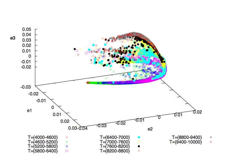
Figures 2 plot the projection of the data onto these first three LLE dimensions. These dimensions are labeled so that $e1$ is the dimension corresponding to the smallest retained eigenvalue of the matrix (3), $e2$ is the dimension corresponding to the second-smallest retained eigenvalue, and so on. Spectra are sorted according to classifications found by comparing DR7 to the SIMBAD database.

Figure 2: Figure 2 plots the SDSS stellar spectra in the first three projected LLE dimensions. Coordinates are named such that $e1$ corresponds to the first coordinate of the LLE decomposition. $e3$ corresponds to the third. Object classifications in the legend derive from the SIMBAD database (http://cds.u-strasbg.fr/cgi-bin/Otype?X). Figure 2 shows the same plot in only the $e1$ and $e2$ coordinates and zoomed in to accentuate the structures formed by emission line galaxies and cataclysmic variables.

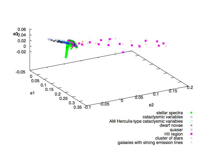
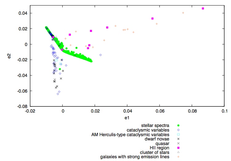
Most objects cluster in a quasi-parabolic feature in the $e1<0.05$, $e2<0$ region of this coordinate space. We will hereafter refer to this feature as the “stellar locus.” The most remarkable feature of this locus is that it appears as a one parameter sequence that is consistent with the classification of spectra by temperature. Notable exceptions are two independent branches: one formed mostly of galactic emission-line spectra that accidentally escaped our initial filtering of the data and one formed of Cataclysmic Variables and Dwarf Novae.

Figure 3: Figure 3 plots example spectra from the galaxy branch in Figure 2. The quantity ds is the distance of the corresponding data point from the stellar locus in $\{e1,e2,e3\}$ space. The flux axis is logarithmic to show both the extreme emission features and the apparent dependence of ds on the continuum. Figure 3 plots example spectra from the CV/DN branch in Figure 2.

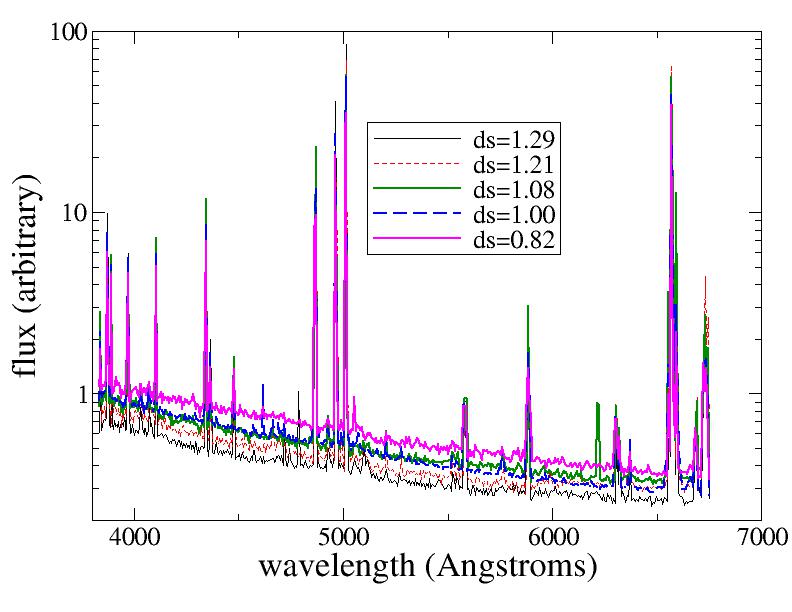
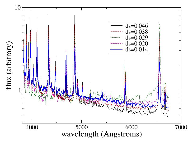
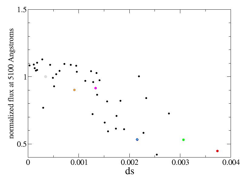
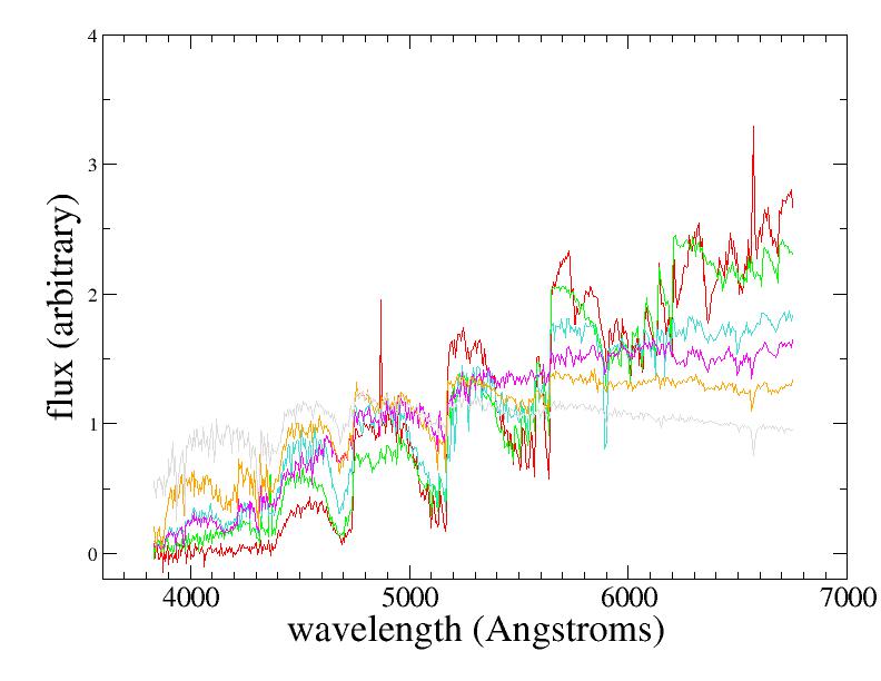
Figure 2 plots the LLE projection in only two dimensions. We see that the galaxy branch extends primarily in the $e1$ direction, while the Cataclysmic Variable/Dwarf Nova branch is nearly parallel to the $e2$ direction. This would seem to indicate that these two projected coordinates correspond to features that dominate in these two classes of objects. Figures 3 and 3 plot example spectra taken from along these branches in LLE space. In both cases, the spectra are dominated by strong emission line features. The quantity ds labelling each of the spectra is their distance in LLE space from the stellar locus. Inspection of Figure 3 reveals that, along the galaxy branch, ds correlates with both the intensity in continuum and line emission. In the case of the CV/DN branch, it is not clear that there is any correlation between ds and the continuum. However, the strengths of many different emission features do correlate with ds, as is shown in Figure 3.

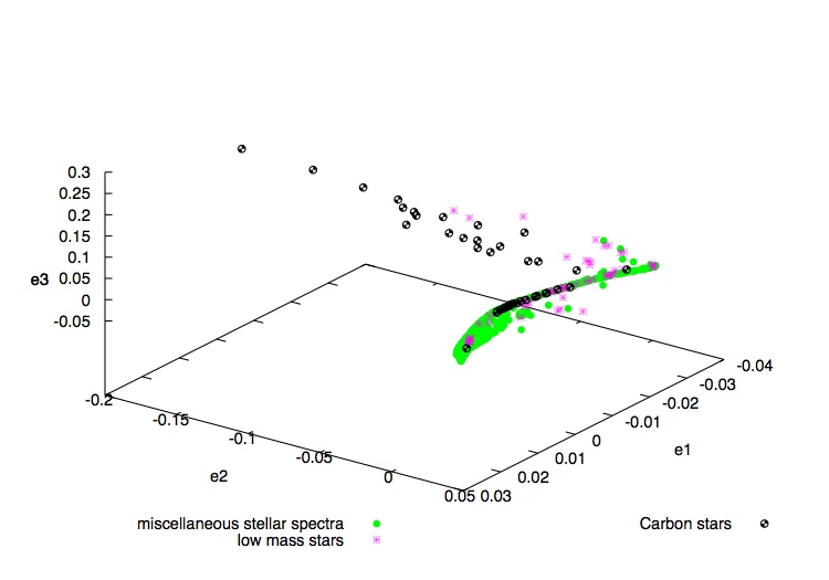
Removing the data points along these branches from the data set and re-performing our analysis, we find that the same quasi-parabolic stellar locus persists, but much more closely confined to a plane in $e1$ and $e2$, while, in this new projection, carbon stars extend far into the $e3$ direction. We present this result in Figure 4. Figure 5 plots examples of carbon star spectra. They seem to be characterized according to the presence or absence of broad absorption features, e.g. at $\sim 5100~{}\AA$.

There is, therefore, a natural progression in the LLE decompositions of the stellar spectra. Deviations from a smooth continuum (e.g. strong emission lines or broad absorption features) perturb the positions of sources away from the “stellar locus” and are identified as outliers within the LLE projected space. Excluding spectra with these emission or absorption features from the projection enables spectra with weaker features to be identified until we are left with a low dimensional series of continuum only stellar spectra. This approach provides both a mechanism for identifying anomalous spectra and for classifying the normal populations.

Figure 6 plots the stellar locus of the original projection from Figure 2 in just two dimensions ($e1$ and $e3$). Looking at the $e1>0$ leg of the stellar locus in this plot, one sees that, even in the original LLE projection, Carbon stars are significantly scattered away from the locus. This is quantified in Figure 5, where the quantity ds is an object’s distance from the stellar locus in Figure 2. We again see a correlation with flux in the feature at $\sim 5100~{}\AA$. We will revisit this parallel between the projections in Figures 2 and 4 in Section V.2.

Figure 4: The first three LLE-projected dimensions of our data set with those objects that exist in the emission line galaxy and CV/DN branches of Figure 2 removed. The stellar locus is now more closely confined to the $e1$ and $e2$ dimensions. Carbon stars extend into the $e3$ dimension.

Figure 5: Figure 5 plots flux in the one broad emission feature versus distance from the stellar locus in Figure 2. Colored points correspond to the example spectra plotted in Figure 5. These figures show only spectra positively identified as carbon stars.

Figure 6: Figure 2 plotted in the $e1$ and $e3$ coordinates to highlight the structure of the stellar locus. The $e1<0$ half of the plot shows a separate branch beneath the stellar locus. This branch is made up primarily of white dwarfs and high proper motion stars.

Figure 7: We compare average spectra along the $e1<0$ section of the stellar locus and the separate White Dwarf branch in Figure 6. Solid (black) curves correspond to spectra that are closer to the White Dwarf branch than the main stellar locus. Dashed (red) curves correspond to spectra that are closer to the stellar locus than the White Dwarf branch. From bottom to top, curves correspond to averages about $e1=-0.01,-0.008,-0.006$.

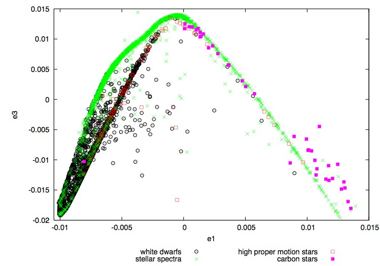
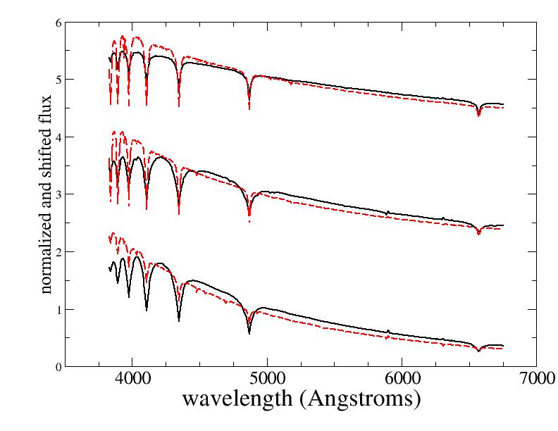
LLE projection also produces some useful substructures within the stellar locus. From the overhead perspective of Figure 2, the stellar locus looks effectively one-dimensional. The same is evident in the two-dimensional projection of Figure 6. The only exception is a bifurcation in the $e1<0$ region. Here, the White Dwarfs and high proper motion stars have separated themselves out into their own branch independent (and below in this projection) of that occupied by other stellar classes. In Figure 7, we segregate the $e1<0$ data points from Figure 6 into two groups: those closer to the White Dwarf branch than the stellar locus, and those closer to the stellar locus. We then average the spectra with similar $e1$-coordinate values and plot them on top of each other. We find that the principal difference between spectra in the White Dwarf branch and spectra in the stellar locus occurs in the continuum flux at short wavelengths. This is consistent with our supposition that the stellar locus is a continuum-dominated feature of our projection.

IV.2 Spectral Classification Using LLE

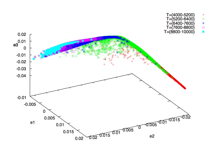
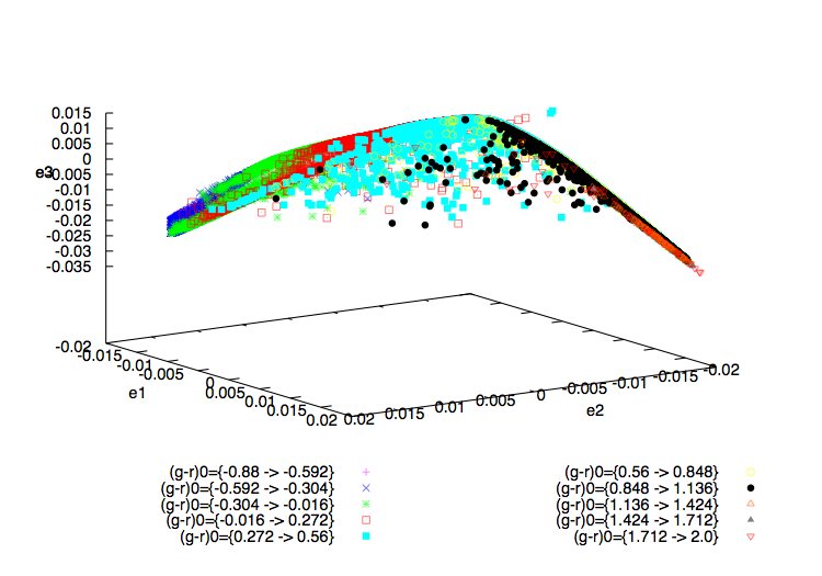
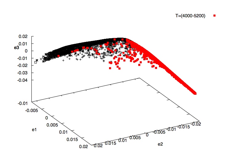
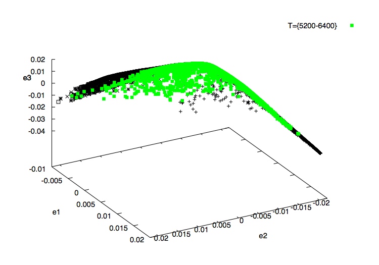
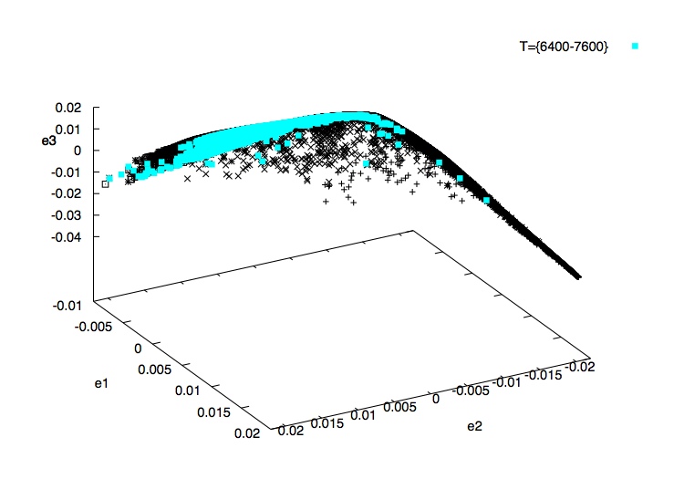
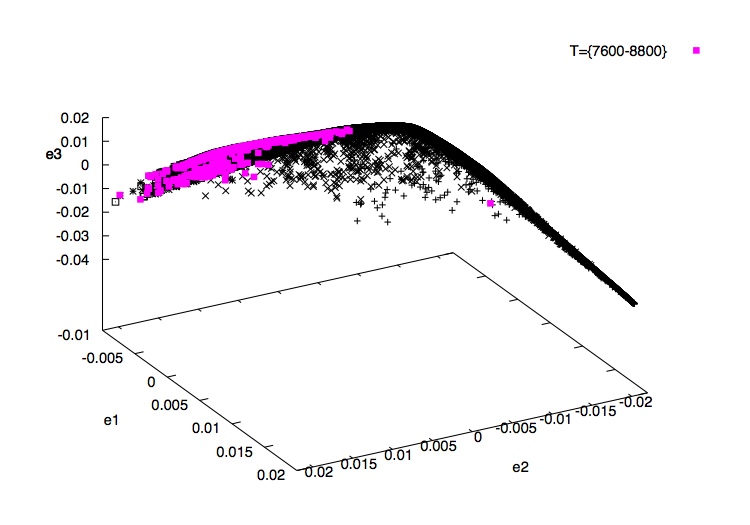
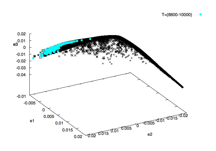
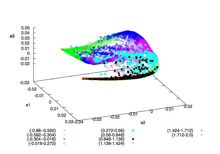
Given the amount of work (see Section II) that has gone into using PCA to automatically classify stars according to their physical properties, it is natural to wonder if LLE could be used to accomplish the same task. Figure 8 plots the stellar locus of Figure 2, but this time sorts the objects by effective temperature (as determined independently by the SDSS sppparams pipeline; data accessible from the SDSS CasJobs site). Tracing along the stellar locus from left to right in that figure, one moves from high to low temperature. Figure 9 reveals the details of this structure by plotting the temperature bins from Figure 8 one at a time. While extremely high and low temperatures are confined to specific regions in the stellar locus, mid-range temperatures exist throughout the entire superstructure. Figure 8 shows the same plot as Figure 8 except that objects are now binned according to $(g-r)_{0}$ color.

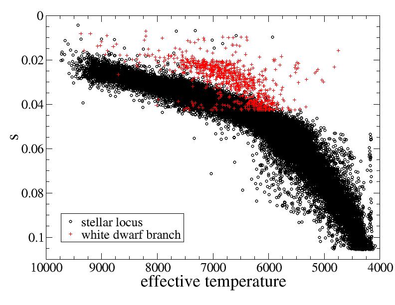
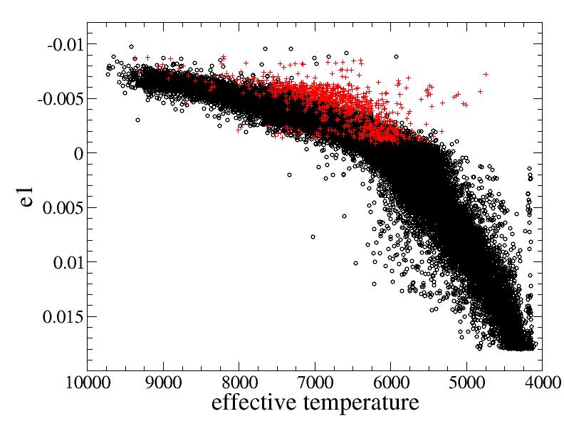
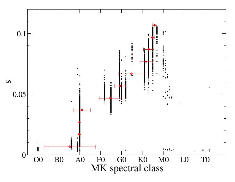
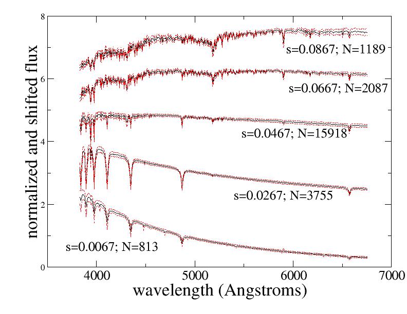
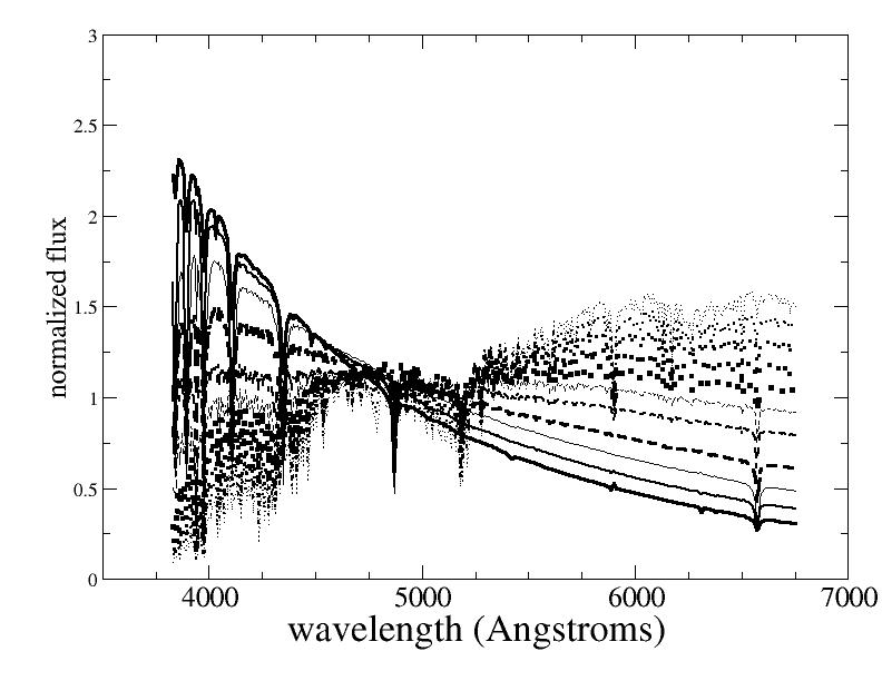
To get a better sense of the spread in effective temperature along the stellar locus, we want to look at the temperature of spectra as a function of their position along the locus. To do this, we require a quantitative means of determining which points are “on the stellar locus,” which points are “on the White Dwarf branch,” and which points are neither. To this end, we parametrize both the stellar locus and the White Dwarf branch as a series of piece-wise $\mathcal{O}(0)$ continuous polynomials in $e1,e2,e3$. A point is “on the stellar locus” if its distance in $e1,e2,e3$ from the parametrized curve is less than $0.001$ and is smaller than its distance to the White Dwarf branch (this gives 43,300 of the original 49,529 spectra). The opposite is true for objects classified as “on the White Dwarf Branch” (giving 4900 spectra). Figure 10 plots the effective temperature of objects on the stellar locus against $s$, their distance along the locus with $s=0$ being at the $e1=-0.0102$ end of the locus (see Figure 6). The axes have been arranged and inverted to highlight the parallels between this plot and the main sequence of the Hertzsprung-Russell diagram. White Dwarfs (the red crosses) cluster above the “main sequence” (rather than below, as in the HR diagram) when their temperatures are plotted against distance along the White Dwarf branch. Figure 11 plots the average spectra in $\Delta s=0.01$ bins along the stellar locus. The spectra are artificially offset to make them more visible. The dashed (red) curves show the $\pm 1~{}\sigma$ spectra about the mean. Figure 12 plots just the mean spectra in that same binning scheme without any offset or error measurement. Because of the correlation between $s$ and temperature, the spectra pivot about a wavelength of $\sim 4800~{}\AA$. This is reminiscent of the observation of Beauchemin et al. (1991) that “[the first eigencomponent in their PCA analysis] weighs equally, but with an opposite sign, the spectra on each side of…$4300~{}\AA$.” They also found that this first eigencomponent correlated with temperature. However, they needed to include a second eigencomponent in order to accurately classify late-type stars. This is not the case for LLE. One dimension (either $s$ or $e1$) is adequate to classify all types of stars, as we show below.

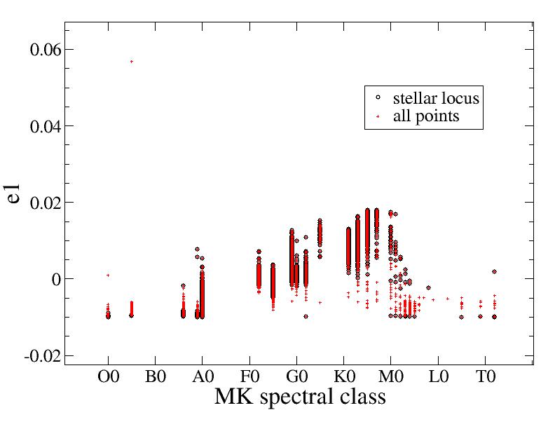
Figure 10 is effectively the same as figure 10, except, instead of the distance $s$ along the stellar locus, the vertical axis is just the $e1$ coordinate of the projected spectra. The qualitative structure of the plot is largely unchanged. Figures 10 and 10 swap MK spectral class for effective temperature and give the same plots (in this case, black circles are stellar locus points; red crosses are all points). In all four cases, there is a strong, monotonic correlation between temperature or spectral class and $s$ or $e1$. This is especially interesting given the findings of previous works that spectral classification using PCA requires at least two eigenspectra to attain any reasonable accuracy Singh et al. (1998, 2001); Storrie-Lombardi et al. (1994); Whitney 1983a ; Whitney 1983b ; Christian (1982). In the words of Singh et al. (2001), this is because “Spectral type has a complex dependence on spectral features, whereas the [Principal Components] are just linearly related to the original spectra” (see especially their Figure 6). By accounting for the non-linear relationships between neighborhoods of spectra, LLE seems to have overcome this hurdle.

Figure 8: The same as Figure 2 except that now objects are classified according to effective temperature (8) and $(g-r)_{0}$ color (8). As you can see, one-dimensional position in the stellar locus correlates well with effective temperature (there are no available effective temperatures or colors for objects far from the stellar locus).

(a) $4000<T_{\text{eff}}<5200$

(b) $5200<T_{\text{eff}}<6400$

(c) $6400<T_{\text{eff}}<7600$

(d) $7600<T_{\text{eff}}<8800$

(e) $8800<T_{\text{eff}}<10000$

Figure 9: The same as Figure 8 with each effective temperature bin plotted separately to show that temperatures are not segregated in the LLE projection space so much as they are layered.

Figure 10: Figure 10 plots effective temperatures versus $s$, the distance along features in Figure 2. The (black) circles are objects on the stellar locus; $s$ is the distance along the locus. The (red) crosses are objects on the White Dwarf branch in Figure 6; $s$ is the distance along the White Dwarf branch. Figure 10 plots effective temperature as a function of the coordinate $e1$ (see Figure 2) for all objects. Figures 10 and 10 show the same plots, substituting spectral classification for effective temperature. Crosses (red) are all objects. The horizontal error bars in Figure (10) are the result of averaging the spectral types in bins of width $\Delta s=0.01$;

Figure 11: We plot the average spectra in bins of width $\Delta s=0.01$ where $s$ is the distance along the stellar locus in Figure 2. Solid (black) curves indicate the mean flux at that wavelength. Dashed (red) curves indicate the $1~{}\sigma$ bounds. $N$ indicates how many spectra were averaged over.

Figure 12: We plot the mean spectra in each of the $\Delta s=0.01$ bins from Figure 11, leaving out the artificial offset that separated the spectr in that plot. The thickest solid curve is the bin centered on $s=0.005$. The thinnest dotted curve is the bin centered on $s=0.095$. The other curves are the intervening bins in monotonic order.

V Discussion and Conclusions

The results of section IV demonstrate the efficacy of LLE as an automatic stellar classification algorithm. In the sections below, we will directly compare LLE to PCA-based methods and propose a more detailed implementation of LLE for future data sets.

V.1 Comparison to PCA

Figures 2 and 6 of this work show the efficacy of LLE at separating spectra by the physical nature (e.g. galaxy, variable star, white dwarf, main sequence star, etc.) of the emitting object. Cabanac et al. (2002) demonstrated a similar utility of PCA however, comparing our figures with their Figure 15, we see that LLE provides a much more straightforward and identifiable division of objects.

From Figures 10 of this work, we see that LLE is also useful for separating out more detailed physical characteristics (i.e. effective temperature and spectral classification) of objects. This has been a major goal of PCA work for several decades. Figure 3(d) of Storrie-Lombardi et al. (1994) shows the efficacy of PCA projection fed into a neural network as a means of accurately reproducing the MK classification of stellar spectra. Their automated classification is arguably more accurate than what you might infer from our Figures 10. However, they require five eigencomponents to achieve that accuracy. Conversely, the correlation between MK classification and LLE projection is largely one dimensional. This is especially evident from our Figure 10, which shows that, without any additional processing, the $e1$ LLE dimension monotonically maps onto MK spectral classification. This mapping is accurate to within a few spectral sub-types. This is the same accuracy achieved with PCA. Recall that we search specifically for a one-dimensional classification scheme. The simplicity of this objective directly limits the accuracy with which we can hope to classify our objects. It is an improvement over the more complex schemes derived from PCA. Christian (1982) attempted to directly reproduce the MK classification using Principal Components. Results from that paper showed that, while the first eigencomponent correlated with spectral type, the correlation was nonlinear, requiring the data set to be divided into early- and late-type stars, each set being analyzed separately. Such nonlinearity is not apparent in our Figure 10. LLE is robust against nonlinearities in the data.

McGurk et al. (2010) showed a correlation between PCA projection and the metallicity of stars. We attempted a similar analysis and found no obvious correlation between LLE dimensions and metallicity.

V.2 Recursive LLE

The progression from Figures 2 to Figure 4 suggests a hierarchical system of layered LLE projections in which each successive projection discards the extreme outliers from its immediate predecessor. That is to say, in the same way that we discarded the galaxy and CV branches identified in Figures 2 to generate Figure 4, we can perform another projection, this time additionally discarding those objects that lie in the carbon star branch ($e2<0$, $e3\rightarrow\infty$) in Figure 4. Figures 13 plot this projection by both effective temperature and color. In this projection, the stellar locus (recall that we have now removed all of the points that do not lie on the stellar locus in Figure 2) is no longer one-dimensional, and, while the progression in temperature (Figure 13) first observed in Figure 8 remains, it is not nearly as clean as the progression in color (Figure 13). By removing the outlier populations, we have allowed more subtle relationships between temperature and color to manifest themselves in the LLE projection. One can imagine continuing this process indefinitely, refining the information gleaned from LLE with each new projection.

Figure 13: The LLE projection of our data with the galaxy and CV branches from Figure 2 and the carbon star branch from Figure 4 excised. Figure 13 color codes the data points according to effective temperature. Figure 13 color codes the data points according to $(g-r)_{0}$ color.