Cluster update for tensor network states

Abstract

We propose a novel recursive way of updating the tensors in projected entangled pair states by evolving the tensor in imaginary time evolution on clusters of different sizes. This generalizes the so-called simple update method of Jiang et al. [Phys. Rev. Lett. 101, 090603 (2008)] and the updating schemes in the single layer picture of Pižorn et al. [Phys. Rev. A 83, 052321 (2011)]. A finite-size scaling of the observables as a function of the cluster size provides a remarkable improvement in the accuracy as compared to the simple update scheme. We benchmark our results on the hand of the spin 1/2 staggered dimerized antiferromagnetic model on the square lattice, and accurate results for the magnetization and the critical exponents are determined.

Numerical simulation of strongly correlated quantum systems in dimension above 1 remains one of the big challenges in condensed matter physics. Quantum monte carlo fails for models suffering from the sign problem, and the density matrix renormalization group method (DMRG) has a problem in 2D because the violation of the area law of entanglement entropy valentinadvphys . Tensor network states (TNSs) nishino-pre64-016705 ; frank04 ; vidal08 , on the other hand, naturally generalize MPSs to higher dimensions and fulfill the area law of entanglement entropy, and are proving to provide powerful tools to simulate problems in above 1 dimension murg ; orus ; jordan ; evenbly ; corboz ; gu ; zhou ; xiang ; su ; kao ; sandvik ; fermiontns .

One of the major difficulties in a TNS algorithm is the scaling of the computational demands as a function of the virtual bond dimension $D$. Inspired by the DMRG algorithm, where truncation is made with respect to the reduced density matrix, a contraction algorithm at the wavefunction level was recently proposed  iztok . However, the rapidly growing renormalized physical index with the system size causes a barrier that hampers the efficiency of the algorithm. The simple update xiang08 , proposed as a generalization of the infinite time-evolving block decimation (iTEBD) algorithm vidal07 to TNSs, successfully avoids the exponentially large Hilbert space, and is very efficient xiang ; su ; ling ; linprb84 . However, the product environment is too simple to capture the long range entanglement and correlations near the critical point of a second order phase transition linprb84 ; su . The efficiency of the simple update still sheds light at controlling the Hilbert space in the complete contraction algorithm iztok . The goal of this paper is to demonstrate that those methods can be merged together in such a way that the advantages of both methods are preserved.

Method – The wavefunction of an infinite projected entangled pair state (iPEPS) in terms of local tensors on 2 sites in the simple update xiang08 is given by

$$|\psi\rangle = \sum_{s_{a},s_{b}}\sum_{ijklmnp}(\Lambda_{ii}\Lambda_{jj}\Lambda_{kk}\Lambda_{mm}\Lambda_{nn}\Lambda_{pp})^{\frac{1}{2}}$$ (1)

$$\times T^{s_{a}}_{ijkl}T^{s_{b}}_{lmnp}|s_{a}\rangle\otimes|s_{b}\rangle\otimes|s_{E}\rangle,$$

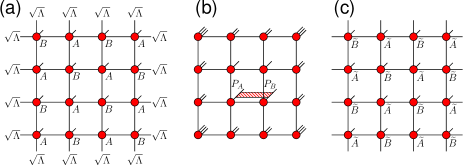
where $|s_{E}\rangle=|i,j,k,m,n,p\rangle$ represents the environmental degrees of freedom. We generalize this construction to a block of $l_{x}\times l_{y}$ sites with the open virtual bonds weighted by the diagonal tensors $\sqrt{\mathbf{\Lambda}}$s, where $\mathbf{\Lambda}$s are the entanglement spectra with respect to each bond, as in Fig. 1(a). As a consequence, the infinite Hilbert space is reduced to the product space of the open virtual bonds and the remaining physical bonds in the cluster as Fig. 1(b). The long range entanglement is gradually considered by taking larger block sizes. Due to the modification of the boundary sites of the cluster, an iPEPS wavefunction is converted to an open boundary (OB) PEPS of size $l_{x}\times l_{y}$, of which the contraction can be done efficiently at the wavefunction level. This conversion is only made at the evolution stage. Once the ground state tensors are obtained, one evaluates expectation values such as the energy and magnetization using the Monte Carlo sampling technique ling to a system with periodic boundary (PB) condition and of system size $L\times L$.

The iterative steps of the cluster update are:

• write the iPEPS wavefunction into an OB PEPS using the $\mathbf{\Lambda}$s from the previous iterations as Fig. 1(a),

• act with a local (imaginary time) evolution operator on several sites located in the center of the $l_{x}\times l_{y}$ cluster as Fig. 1(b),

• contract every virtual bond except the one with the evolution operator, obtain the projectors and a new $\mathbf{\Lambda}$ as discussed below, and project the enlarged bond back to $D$,

• finally replace the iPEPS wavefunction by the updated tensors as Fig. 1(c), and move to a different bond.

There are two main choices to be made in the above update procedure: first of all, how to contract the environment tensor efficiently to two sites under the time evolution; second, how to obtain the updated tensor.

Figure 1: (a) Wavefunction of an infinite lattice in terms of $l_{x}\times l_{y}$ local tensors and the entanglement spectra placed on each open bond. (b) An equivalent OB PEPS to (a), with 2 sites acted by evolution operator in the center of the cluster. (c) After projection with projectors $\mathbf{P}_{A},\mathbf{P}_{B}$, and replace $\mathbf{A,B}$ with $\widetilde{\mathbf{A}},\widetilde{\mathbf{B}}$ everywhere, a new iPEPS wavefunction is obtained.

Figure 2: (a) MPSs $|\rho_{b}\rangle$ and $|\rho_{t}\rangle$ of a conventional contraction method dealing with the norm $\langle\psi|\psi\rangle$ of a wavefunction $|\psi\rangle$, (b) MPSs $|\phi_{b}\rangle$ and $|\phi_{t}\rangle$ of a novel contraction method dealing with the wavefunction $|\psi\rangle$ directly.

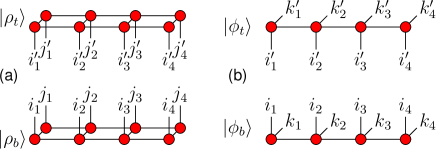
To answer the first question, let us remind the conventional way of contracting the environment tensor. In the conventional evolution methods, one constructs a double tensor network, which represents the norm $\langle\psi|\psi\rangle$ of the state $|\psi\rangle$, then contracts this norm to obtain the environment tensor of two sites. The major approximation is to represent the bottom (top) rows of the norm by an MPS: $|\rho_{b}(\bar{i},\bar{j})\rangle\equiv\mbox{Tr}_{\bar{k}}\langle\phi_{b}(\bar{i},\bar{k})|\phi_{b}(\bar{j},\bar{k})\rangle$ ($|\rho_{t}(\bar{i}^{\prime},\bar{j}^{\prime})\rangle\equiv\mbox{Tr}_{\bar{k^{\prime}}}\langle\phi_{t}(\bar{i^{\prime}},\bar{k^{\prime}})|\phi_{t}(\bar{j^{\prime}},\bar{k^{\prime}})\rangle$) as Fig. 2(a), where $|\phi_{b}(\bar{i},\bar{k})\rangle$ ($|\phi_{t}(\bar{i}^{\prime},\bar{k}^{\prime})\rangle$) is the wavefunction of the bottom (top) rows with the highest (lowest) vertical bonds open, as Fig. 2(b), $\bar{i}\equiv\{i_{1},i_{2},i_{3},i_{4}\}$, etc. However, during the contraction, one ignores the fact that $|\rho_{b}(\bar{i},\bar{j})\rangle$ is hermitian if written as a density matrix of the fictitious degrees of freedom $\bar{i}$ and $\bar{j}$, and treats $|\rho_{b}(\bar{i},\bar{j})\rangle$ as a general MPS with degrees of freedom $\{i_{l},j_{l}\}$ at each site $l$. This will cause ill-condition if the truncation error is large. We therefore contract the wavefunction directly to ensure the hermiticity of the norm. The degrees of freedom at each site $l$ of $|\phi_{b}(\bar{i},\bar{k})\rangle$ is $\{i_{l},k_{l}\}$ with $i_{l}$ represents the topmost vertical index and $k_{l}$ represents the renormalized physical index of the $l^{\mbox{th}}$ bottom-half-column. The argument for $|\phi_{b}(\bar{i},\bar{k})\rangle$ equally applies to $|\phi_{t}(\bar{i}^{\prime},\bar{k}^{\prime})\rangle$ throughout the paper.

To contract a tensor network wavefunction with OB conditions, one absorbs a row into $|\phi_{b}\rangle$ to obtain $|\widetilde{\phi}_{b}\rangle$, as Fig. 3(a,b). Unlike in the case of contracting the norm, this is described as a matrix product operator (MPO) acting on an MPS, in such a way that not only the internal bond dimension $\chi$ but also the physical degrees of freedom $\tilde{d}$ of $|\phi_{b}\rangle$ is increased by a factor of $D$ and $d$ respectively as Fig. 3(b), where $D$ and $d$ are the virtual bond dimension and the physical degrees of freedom in the original lattice. In order to keep the renormalization under control, one has to truncate both, as Fig. 3(c).

Figure 3: (a) Renormalize a row into the MPS $|\phi_{b}\rangle$. (b) Absorb a row into $|\phi_{b}\rangle$ enlarges both the internal bond and the physical bond by a factor $D$ and $d$ respectively. (c) Projectors (blue triangles) $\mathbf{P}^{i}_{L}$, $\mathbf{P}^{i}_{R}$ and $\bar{\mathbf{P}}^{i}_{S}$ is calculated to reduce both the internal bond and physical bond of matrix $\mathbf{M}^{i}$.

Figure 4: (a-d) Calculate the residue matrix (blue diamonds) $\mathbf{R_{i}}$ ($\mathbf{L_{i}}$) of the left (right) half chain up to site $i$ by iteratively using QR (LQ) decompositions. (e) Replace left (right) half chain by $\mathbf{R}^{i}$ ($\mathbf{L}^{i+1}$) and use an SVD to reduce the dimension of the $i$-th bond. (f) Inserted an identity (hollow diamond) at bond $i$ in original MPS and replace $\mathbf{R}^{i}\mathbf{L}^{i+1}\approx\bar{\mathbf{U}}\bar{\mathbf{\Sigma}}\bar{\mathbf{V}}^{\dagger}$ to obtain the projectors $\mathbf{P}^{i}_{R}$ and $\mathbf{P}^{i+1}_{L}$.

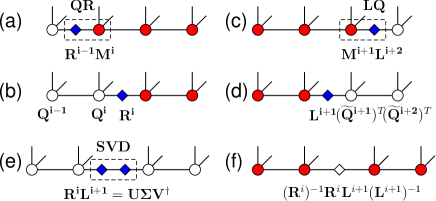
To reduce the bond dimension between site $i$ and $i+1$ of an OB MPS, a singular value decomposition (SVD) is done on $|\widetilde{\phi}_{b}\rangle$. As in Fig. 3(e), one needs the right (left) residue matrix $\mathbf{R}^{i}$ ($\mathbf{L}^{i+1}$) of the left (right) half chain up to the site $i$ ($i+1$) to bring them into their normal form valentinadvphys . To be specific, one calculates the boundary residue matrix $\mathbf{R}^{1}$ ($\mathbf{L}^{n}$) using a QR (LQ) decomposition, $n$ is the length of $|\widetilde{\phi}_{b}\rangle$,

$$M^{1}_{usr}=\sum_{r^{\prime}}Q^{1}_{us,r^{\prime}}R^{1}_{r^{\prime},r},$$ (2)

$$M^{n}_{lus}=\sum_{l^{\prime}}L^{n}_{l,l^{\prime}}(\widetilde{Q}^{n}_{l^{\prime},us})^{T},$$ (3)

then moves one site to the right (left) as in Fig. 4(a-d),

$$\sum_{l^{\prime}}R^{i-1}_{l,l^{\prime}}M^{i}_{l^{\prime},usr}=\sum_{r^{\prime}}Q^{i}_{lus,r^{\prime}}R^{i}_{r^{\prime},r},$$ (4)

$$\sum_{r^{\prime}}M^{i}_{lus,r^{\prime}}L^{i+1}_{r^{\prime},r}=\sum_{l^{\prime}}L^{i}_{l,l^{\prime}}(\widetilde{Q}^{i}_{l^{\prime},usr})^{T},$$ (5)

where $\mathbf{M}^{i}$ is the matrix at the site $i$ of $|\widetilde{\phi}_{b}\rangle$, $l,r,u,s$ represent the left, right, up and physical index respectively, and $\mathbf{Q}^{i}$ ($\widetilde{\mathbf{Q}}^{i}$) is isometric matrix. Thus the left (right) half chain, which is replaced by $\mathbf{R}^{i}$ ($\mathbf{L}^{i+1}$), is in its normal form as Fig. 4(e). An SVD $\mathbf{R}^{i}\mathbf{L}^{i+1}\approx\bar{\mathbf{U}}\bar{\mathbf{\Sigma}}\bar{\mathbf{V}}^{\dagger}$ will minimize $||\widetilde{\phi}_{b}\rangle-|\phi_{b}^{\prime}\rangle||^{2}$, where $|\phi_{b}^{\prime}\rangle$ is the one-bond reduced MPS to $|\widetilde{\phi}_{b}\rangle$, bar means taking the leading singular values or vectors. To derive the projectors for this reduction, one inserts an identity $(\mathbf{R}^{i})^{-1}\mathbf{R}^{i}\mathbf{L}^{i+1}(\mathbf{L}^{i+1})^{-1}$ at bond $i$ in the original MPS and substitutes $\mathbf{R}^{i}\mathbf{L}^{i+1}$ by $\bar{\mathbf{U}}\bar{\mathbf{\Sigma}}\bar{\mathbf{V}}^{\dagger}$ as Fig. 4(f). Equally distributing $\bar{\mathbf{\Sigma}}$ to each side, one writes the projectors at bond $i$ as

$$\mathbf{P}^{i}_{R}=(\mathbf{R}^{i})^{-1}\mathbf{\bar{U}}\sqrt{\mathbf{\bar{\Sigma}}},\quad(\mathbf{P}^{i+1}_{L})^{T}=\sqrt{\mathbf{\bar{\Sigma}}}\mathbf{\bar{V}}^{\dagger}(\mathbf{L}^{i+1})^{-1}.$$ (6)

To avoid the matrix inversion, one can use $(\mathbf{R}^{i}\mathbf{L}^{i+1})^{-1}=\mathbf{V}\frac{1}{\mathbf{\Sigma}}\mathbf{U}^{\dagger}$ to rewrite the projectors as

$$\mathbf{P}^{i}_{R}=\mathbf{L}^{i+1}\mathbf{\bar{V}}\frac{1}{\sqrt{\mathbf{\bar{\Sigma}}}},\quad(\mathbf{P}^{i+1}_{L})^{T}=\frac{1}{\sqrt{\mathbf{\bar{\Sigma}}}}\mathbf{\bar{U}}^{\dagger}\mathbf{R}^{i};$$ (7)

note that taking $\mathbf{\bar{\Sigma}}^{-1}$ will not cause a singularity as the small singular values are discarded. To reduce the physical degrees of freedom of $\mathbf{M}^{i}$, one considers the reduced density matrix $\rho^{i}_{s,s^{\prime}}$ of site $i$ as Fig. 5. Define $\widetilde{M}^{i}_{lusr}=\sum_{l^{\prime}r^{\prime}}R^{i-1}_{l,l^{\prime}}M^{i}_{l^{\prime}usr^{\prime}}L^{i+1}_{r^{\prime},r}$, then $\rho^{i}_{s,s^{\prime}}=\sum_{lur}\widetilde{M}^{i}_{s,lur}\widetilde{M}^{i\dagger}_{lur,s^{\prime}}$. The leading eigenvectors $\bar{\mathbf{P}}^{i}_{S}$ of $\rho^{i}=\mathbf{P}^{i}_{S}\mathbf{\Lambda}^{i}\mathbf{P}^{i\dagger}_{S}$ is the projector to reduce the physical degrees of freedom of $\mathbf{M}^{i}$. Upon obtaining $\mathbf{P}^{i}_{L}$, $\mathbf{P}^{i}_{R}$ and $\bar{\mathbf{P}}^{i}_{S}$, one projects according to Fig. 3(c). Note that one left (right) sweep can obtain $\mathbf{R}^{i}$ ($\mathbf{L}^{i}$) for all sites. It turns out that the reduction of each internal bond and physical bond can be done simultaneously as if they are independent. This concludes the question of the contraction at the single-layer wavefunction level.

Figure 5: (a) Reduced density matrix of the physical bond $s$ at site $i$ of $|\widetilde{\phi}_{b}\rangle$. (b,c) A reformation of (a) by $\mathbf{M}^{i}$ and the left and right residue matrices $\mathbf{L}^{i+1}$, $\mathbf{R}^{i-1}$.

Figure 6: (a) Bottom and top MPS $|\phi_{b}\rangle$, $|\phi_{t}\rangle$ sandwich a row with the evolution operator. (b) Further absorb all columns into the left (right) MPS $|\phi_{l}\rangle$ ($|\phi_{r}\rangle$). (c) Contract all virtual bonds in (b) except $h_{2}$ to form a single tensor $\mathbf{T}$.

Now we focus on the question of how to obtain the evolved tensors using the partially contracted wavefunction. After renormalizing rows from below (above) into $|\phi_{b}\rangle$ ($|\phi_{t}\rangle$) as Fig. 6(a), one renormalizes columns from left (right) into $|\phi_{l}(\bar{h},\bar{s}_{l})\rangle$ ($|\phi_{r}(\bar{h},\bar{s}_{r})\rangle$), as in Fig. 6(b), where the thickened bond is due to the action of the evolution operator. Define

$$|\widetilde{\psi}(\bar{s}_{l},\bar{s}_{r})\rangle=\sum_{\bar{h}}|\phi_{l}(\bar{h},\bar{s}_{l})\rangle\otimes\phi_{r}(\bar{h},\bar{s}_{r})\rangle,$$ (8)

where $\bar{h}=\{h_{1},h_{2},h_{3}\}$ is the horizontal internal bond, the projector to reduce the thickened bond has to minimize the 2-norm $||\widetilde{\psi}(\bar{s}_{l},\bar{s}_{r})\rangle-|\psi^{\prime}(\bar{s}_{l},\bar{s}_{r})\rangle||^{2}$. Unlike in the OB MPS, where one cut will bipartite the wavefunction, here one deals with a ring MPS. We present an empirical way to calculate the projectors. First contract all virtual bonds in $|\widetilde{\psi}(\bar{s}_{l},\bar{s}_{r})\rangle$ except the thickened bond $h_{2}$ to form a single tensor $\mathbf{T}$ as Fig. 6(c); in analogy to an OB MPS, make a QR (LQ) decomposition to calculate the right (left) residue matrix $\mathbf{R}$ ($\mathbf{L}$) of the tensor $\mathbf{T}$ as

$$T_{rs,l}=\sum_{l^{\prime}}Q_{rs,l^{\prime}}R_{l^{\prime},l},$$ (9)

$$T_{r,sl}=\sum_{r^{\prime}}L_{r,r^{\prime}}\widetilde{Q}^{T}_{r^{\prime},sl},$$ (10)

where $\mathbf{Q}$ ($\widetilde{\mathbf{Q}}$) is isometric matrix; insert $\mathbf{R}^{-1}\mathbf{RLL}^{-1}$ between the $l,r$ indices of tensor $\mathbf{T}$, in analogy to Eq. 7, derive the projectors to the imaginary time evolution as

$$\mathbf{P}_{A}=\mathbf{L\bar{V}}\frac{1}{\sqrt{\mathbf{\bar{\Lambda}}}},\quad(\mathbf{P}_{B})^{T}=\frac{1}{\sqrt{\mathbf{\bar{\Lambda}}}}\mathbf{\bar{U}^{\dagger}R},$$ (11)

where an SVD $\mathbf{RL}\approx\bar{\mathbf{U}}\bar{\mathbf{\Lambda}}\bar{\mathbf{V}^{\dagger}}$ is performed. $\bar{\mathbf{\Lambda}}$ for this particular bond contains the entanglement spectrum that replaces the previous one for the next evolution step, analogous to what happens in the simple update scheme. Calculating the $\mathbf{T}$ tensor explicitly is expensive, what one does instead when dealing with the object Fig. 6(c) is treating the $r$ index as the physical ones $\{\bar{s}_{l},\bar{s}_{r}\}$ to calculate the $\mathbf{R}$ matrix and again treating the $l$ index as the physical ones to calculate the $\mathbf{L}$ matrix. Another way to update the projectors $\mathbf{P}_{A}$, $\mathbf{P}_{B}$ would be alternatively solving the multi-quadratic equations valentinadvphys , where the $\mathbf{T}$ tensor is explicitly needed.

Figure 7: (a) Ground state energy errors per site for $L=16$ using tensors of bond dimension $D=5$ obtained via the simple update ($l_{x}=2$) and the cluster update ($l_{x}=4,6,8$).

Figure 8: (a) Sublattice magnetization square for $L=16$ using the same parameters as Fig. 7, black solid line is the SSE results for $L=16$, solid circles are the CSE results from (b). (b) The cluster size extrapolations (CSE) for the finite size ($L=16$) magnetizations using cluster sizes $l_{x}=2,4,6,8$.

Results – We benchmark our method using the spin 1/2 staggered dimerized antiferromagnetic Heisenberg model on square lattice with PB conditions and compare our results to that obtained from the simple update linprb84 , iPEPS method bauerjstatmech and the QMC simulation wenzel . The Hamiltonian is written as

$$H=J\sum_{\langle i,j\rangle}\mathbf{S}_{i}\cdot\mathbf{S}_{j}+J^{\prime}\sum_{\langle\langle k,l\rangle\rangle}\mathbf{S}_{k}\cdot\mathbf{S}_{l},\quad(J,J^{\prime}>0),$$ (12)

where $\langle\langle k,l\rangle\rangle$ are the horizontal nearest neighbor pairs satisfying $\mbox{mod}(x_{k},2)=\mbox{mod}(y_{k},2)$, $x_{k},y_{k}$ is the lattice coordinate of site $k$, $\langle i,j\rangle$ are all other nearest neighbor pairs, and $J,J^{\prime}$ are the coupling strengths. This model is frustration free and has been extensively studied wenzel using the stochastic series expansion (SSE) method sandvikprb56-11678 . Increasing the coupling strength ratio $J^{\prime}/J$ drives the system through a second order phase transition from the antiferromagnetic ordered phase to a magnetically disordered phase. We set $J=1$ for convenience hereafter.

We obtain the finite size ground state energies and the magnetization for systems with linear size $L=4,8,16$. Each system is measured using the variational monte carlo (VMC) sampling technique ling taking the tensors of bond dimension $D=5$ obtained through the cluster update with cluster size $l_{x}\times l_{y}=2\times 1$, $4\times 4$, $6\times 6$ and $8\times 8$. For this specific model, the simple update is equivalent to a cluster update with cluster size $2\times 1$.

Figure 9: (a) Finite size magnetizations and their thermodynamic limits via the FSS from (b), the black solid lines are the SSE simulation results for system size $L=4,8,16$ and the black dash line is their FFS results. (b) Finite size scaling of the magnetization square using system sizes $L=4,8,16$.

Figure 10: Fitting of the magnetization curve for the critical value $J^{\prime}_{c}$ and the critical exponent $\beta$.

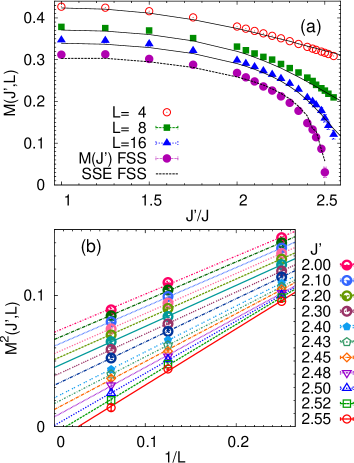
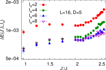
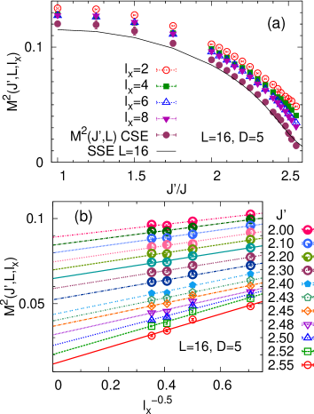
We present the ground state energy errors per site for system size $L=16$ with $D=5$ in Fig. 7 and the sublattice magnetization square defined as following sandvikprb56-11678 in Fig. 8,

$$M^{2}=\frac{1}{L^{2}}\sum_{i}\mathbf{S}_{x_{i},y_{i}}\cdot\mathbf{S}_{x_{i}+\frac{L}{2},y_{i}+\frac{L}{2}}.$$ (13)

Significant improvement in energy and magnetization is achieved by increasing the cluster size $l_{x}$ from 2 to 8. We make a cluster size extrapolation (CSE) for the finite size magnetization in Fig. 8(b) as

$$M^{2}(J^{\prime},L,l_{x})=M^{2}(J^{\prime},L)+a_{J^{\prime}}/\sqrt{l_{x}},$$ (14)

where $M^{2}(J^{\prime},L)$ and $a_{J^{\prime}}$ are the fitting parameters. The CSE results are in good agreement with the finite size magnetization through the SSE simulation, as plotted in Fig. 8(a). Here the cluster size $l_{x}$ plays the role of the bond dimension $D$ to provide a scaling scheme. To obtain the sublattice magnetization in the thermodynamic limit, we use the following finite size scaling (FSS) formula neubergerprb39 ; fisherprb39 ; sandvikprb56-11678 to extrapolate $M(J^{\prime})$ as in Fig. 9(b)

$$M^{2}(J^{\prime},L)=M^{2}(J^{\prime})+b_{J^{\prime}}/L,$$ (15)

where $M^{2}(J^{\prime})$ and $b_{J^{\prime}}$ are the fitting parameters. This FSS formula is only valid for the states with persisting sublattice magnetization, thus the extrapolated negative $M^{2}(J^{\prime})$ simply means that these states have no magnetic order. The finite size magnetizations $M(J^{\prime},L)$ together with their thermodynamic limits $M(J^{\prime})$ are plotted in Fig. 9(a). The extrapolated $M(J^{\prime})$ lies a bit off the SSE FSS results near the critical point, because the latter are fitted with a sub-leading corrections $1/L^{2}$ using system sizes $L=4,8,16,32$. To determine the critical value $J^{\prime}_{c}$ and the critical exponent $\beta$, we fit $M(J^{\prime})$ by

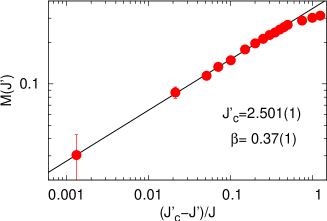
$$M(J^{\prime})=c(J_{c}^{\prime}-J^{\prime})^{\beta},$$ (16)

where $J^{\prime}_{c}$, $\beta$ and $c$ are the fitting parameters, as in Fig. 10. We obtain a critical value $J^{\prime}_{c}=2.501(1)$ and the critical exponent $\beta=0.37(1)$. The SSE results are $J^{\prime}_{c}=2.5198(3)$ and $\beta=0.376(5)$ wenzel . The offset in $J^{\prime}_{c}$ is due to ignoring the sub-leading corrections in the FSS formula Eq. 15. Considering it would require results from a much larger bond dimension $D$ for system size $L=32$. The critical value from the simple update is $J_{c}^{\prime}=2.56$ linprb84 , and from the iPEPS is $J_{c}^{\prime}\approx 2.85$ bauerjstatmech .

discussion – The cluster update allows one to accurately determine the behavior of a second order phase transition using a tensor network state of intermediate bond dimension $D$ and relatively small cluster size $l_{x}$. The simple update is efficient, however it always generates a fat tail near the exact transition point; on the contrary, the cluster update that has been introduced here improves those results significantly. This improvement is especially important when a narrow intermediate phase is present in the phase diagram, such as in the frustrated $J_{1}-J_{2}$ Heisenberg model on square lattice. Comparing to the complete contraction algorithm in  iztok , the Hilbert space is drastically reduced, which significantly boosts the efficiency, and the algorithm is simpler in the sense that it is free of dealing with the boundary evolutions. The cluster update scales as $D^{4}\chi^{2}d\tilde{d}$. The renormalized physical index $\tilde{d}$ varies depending on the entanglement of the state, however it is bounded by $D\chi^{2}$. Choosing a small cluster size also relaxes the scaling of $\tilde{d}$, e.g. the complexity with cluster size $2\times 2$ scales as $D^{5}$, and $4\times 4$ scales as $D^{7}$ if taking $\chi=D$.

Conclusion – We presented a cluster imaginary time evolution method for a tensor network state (TNS) describing the ground state of strongly correlated quantum systems. We benchmarked this method with the staggered dimerized antiferromagnetic Heisenberg model on the square lattice and accurately determined its critical value and critical exponents $\beta$ using a TNS with fairly small bond dimension $D=5$; this provides clear evidence for an improvement over the simple update scheme in  xiang08 . The efficiency and accuracy of this method should allow tensor network simulations to be applied to a zoo of interesting models that are not easily accessible by other methods, especially as large values of $D$ can be treated progress .

Acknowledgments: This project is supported by the EU Strep project QUEVADIS, the ERC grant QUERG, and the FWF SFB grants FoQuS and ViCoM. The computational results presented have been achieved using the Vienna Scientific Cluster (VSC).

References

- (1) F. Verstraete, V. Murg, and J. I. Cirac, Adv. Phys. 57, 143 (2008).
- (2) N. Maeshima, Y. Hieida, Y. Akutsu, T. Nishino, and K. Okunishi, Phys. Rev. E 64, 016705 (2001).
- (3) F. Verstraete and J. I. Cirac, arXiv:cond-mat/0407066v1.
- (4) G. Vidal, Phys. Rev. Lett. 101, 110501 (2008).
- (5) V. Murg, F. Verstraete, and J. I. Cirac, Phys. Rev. Lett. 95, 057206 (2005); V. Murg, F. Verstraete, and J. I. Cirac, Phys. Rev. A 75, 033605 (2007); V. Murg, F. Verstraete, and J. I. Cirac, Phys. Rev. B 79, 195119 (2009); V. Murg, Ö. Legeza, R. M. Noack, and F. Verstraete, Phys. Rev. B 82, 205105 (2010).
- (6) R. Orus, A. C. Doherty, and G. Vidal, Phys. Rev. Lett. 102, 077203 (2009); R. Orus and G. Vidal, Phys. Rev. B. 80, 094403 (2009).
- (7) J. Jordan, R. Orus, G. Vidal, F. Verstraete, and J. I. Cirac, Phys. Rev. Lett. 101, 250602 (2008); J. Jordan, R. Orus, and G. Vidal, Phys. Rev. B 79, 174515 (2009).
- (8) G. Evenbly and G. Vidal, Phys. Rev. Lett. 104, 187203 (2010).
- (9) P. Corboz, J. Jordan, and G. Vidal, Phys. Rev. B 82, 245119 (2010); P. Corboz, S. R. White, G. Vidal, and M. Troyer, Phys. Rev. B 84, 041108 (2011); P. Corboz, A. M. Läuchli, K. Penc, M. Troyer, and F. Mila, arXiv:1108.2857.
- (10) Z.-C. Gu, M. Levin, and X.-G. Wen, Phys. Rev. B 78, 205116 (2008); Z.-C. Gu, arXiv:1109,4470; Z.-C. Gu, H.-C. Jiang, D. N. Sheng, H. Yao, L. Balents, and X.-G. Wen, arXiv:1110.1183.
- (11) Q.-Q. Shi, S.-H. Li, J.-H. Zhao, and H.-Q. Zhou, arXiv:0907.5520; S.-H. Li, Q.-Q. Shi, and H.-Q. Zhou, arXiv:1001.3343.
- (12) H.H. Zhao, Z.Y. Xie, Q.N. Chen, Z.C. Wei, J.W. Cai, and T. Xiang, Phys. Rev. B. 81, 174411 (2010); H. H. Zhao, C. Xu, Q. N. Chen, Z. C. Wei, M. P. Qin, G. M. Zhang, and X. Tao, arXiv:1105.2716.
- (13) W. Li, S. S. Gong, Y. Zhao, and G. Su, Phys. Rev. B 81, 184427 (2010); W. Li, S. S. Gong, Y. Zhao, S. J. Ran, S. Gao, and G. Su, Phys. Rev. B 82, 214431 (2010).
- (14) L. Wang, Y.-J. Kao, and A. W. Sandvik, Phys. Rev. E 83, 056703 (2011); J.-F. Yu and Y.-J. Kao, arXiv:1108.3393.
- (15) C. Liu, L. Wang, A. W. Sandvik, Y.-C. Su, and Y.-J. Kao, Phys. Rev. B 82, 060410R (2010); C. Liu, D.-X. Yao, and A. W. Sandvik, arXiv:1110.0761.
- (16) C. V. Kraus, N. Schuch, F. Verstraete, and J. I. Cirac, Phys. Rev. A 81, 052338 (2010); P. Corboz, R. Orus, B. Bauer, and G. Vidal, Phys. Rev. B 81, 165104 (2010); Z.-C. Gu, F. Verstraete, and X.-G. Wen, arXiv:1004.2563; I. Pižorn and F. Verstraete, Phys. Rev. B 81, 245110 (2010).
- (17) I. Pižorn, L. Wang, and F. Verstraete, Phys. Rev. A 83, 052321 (2011).
- (18) H. C. Jiang, Z. Y. Weng, and T. Xiang, Phys. Rev. Lett. 101, 090603 (2008).
- (19) G. Vidal, Phys. Rev. Lett. 98, 070201 (2007).
- (20) L. Wang, I. Pižorn, and F. Verstraete, Phys. Rev. B 83, 134421 (2011).
- (21) C.-Y. Huang and F.-L. Lin, Phys. Rev. B 84, 125110 (2011).
- (22) B. Bauer, G. Vidal, and M. Troyer, J. Stat. Mech. 2009, P09006.
- (23) S. Wenzel, L. Bogacz, and W. Janke, Phys. Rev. Lett. 101, 127202 (2008).
- (24) A. W. Sandvik, Phys. Rev.B 56, 11678 (1997).
- (25) H. Neuberger and T. Ziman, Phys. Rev. B 39, 2608 (1989).
- (26) D. S. Fisher, Phys. Rev. B 39, 11783 (1989).
- (27) L. Wang et al., Work in Progress.