Discovering Emerging Topics in Social Streams via Link Anomaly Detection

Abstract

Detection of emerging topics are now receiving renewed interest motivated by the rapid growth of social networks. Conventional term-frequency-based approaches may not be appropriate in this context, because the information exchanged are not only texts but also images, URLs, and videos. We focus on the social aspects of theses networks. That is, the links between users that are generated dynamically intentionally or unintentionally through replies, mentions, and retweets. We propose a probability model of the mentioning behaviour of a social network user, and propose to detect the emergence of a new topic from the anomaly measured through the model. We combine the proposed mention anomaly score with a recently proposed change-point detection technique based on the Sequentially Discounting Normalized Maximum Likelihood (SDNML), or with Kleinberg’s burst model. Aggregating anomaly scores from hundreds of users, we show that we can detect emerging topics only based on the reply/mention relationships in social network posts. We demonstrate our technique in a number of real data sets we gathered from Twitter. The experiments show that the proposed mention-anomaly-based approaches can detect new topics at least as early as the conventional term-frequency-based approach, and sometimes much earlier when the keyword is ill-defined.

Keywords: Topic Detection, Anomaly Detection, Social Networks, Sequentially Discounted Maximum Likelihood Coding, Burst detection

1 Introduction

Communication through social networks, such as Facebook and Twitter, is increasing its importance in our daily life. Since the information exchanged over social networks are not only texts but also URLs, images, and videos, they are challenging test beds for the study of data mining.

There is another type of information that is intentionally or unintentionally exchanged over social networks: mentions. Here we mean by mentions links to other users of the same social network in the form of message-to, reply-to, retweet-of, or explicitly in the text. One post may contain a number of mentions. Some users may include mentions in their posts rarely; other users may be mentioning their friends all the time. Some users (like celebrities) may receive mentions every minute; for others, being mentioned might be a rare occasion. In this sense, mention is like a language with the number of words equal to the number of users in a social network.

We are interested in detecting emerging topics from social network streams based on monitoring the mentioning behaviour of users. Our basic assumption is that a new (emerging) topic is something people feel like discussing about, commenting about, or forwarding the information further to their friends. Conventional approaches for topic detection have mainly been concerned with the frequencies of (textual) words [1, 2]. A term frequency based approach could suffer from the ambiguity caused by synonyms or homonyms. It may also require complicated preprocessing (e.g., segmentation) depending on the target language. Moreover, it cannot be applied when the contents of the messages are mostly non-textual information. On the other hands, the “words” formed by mentions are unique, requires little prepossessing to obtain (the information is often separated from the contents), and are available regardless of the nature of the contents.

Figure 1 shows an example of the emergence of a topic through posts on social networks. The first post by Bob contains mentions to Alice and John, which are both probably friends of Bob’s; so there is nothing unusual here. The second post by John is a reply to Bob but it is also visible to many friends of John’s that are not direct friends of Bob’s. Then in the third post, Dave, one of John’s friends, forwards (called retweet in Twitter) the information further down to his own friends. It is worth mentioning that it is not clear what the topic of this conversation is about from the textual information, because they are talking about something (a new gadget, car, or jewelry) that is shown as a link in the text.

Figure 1: Example of the emergence of a topic in social streams.

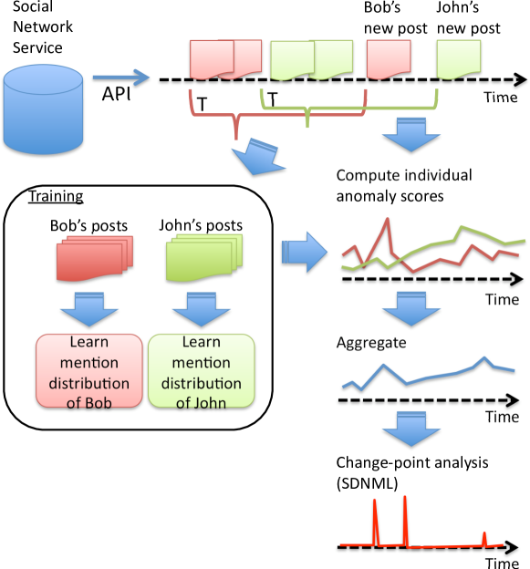
In this paper, we propose a probability model that can capture the normal mentioning behaviour of a user, which consists of both the number of mentions per post and the frequency of users occurring in the mentions. Then this model is used to measure the anomaly of future user behaviour. Using the proposed probability model, we can quantitatively measure the novelty or possible impact of a post reflected in the mentioning behaviour of the user. We aggregate the anomaly scores obtained in this way over hundreds of users and apply a recently proposed change-point detection technique based on the Sequentially Discounting Normalized Maximum Likelihood (SDNML) coding [3]. This technique can detect a change in the statistical dependence structure in the time series of aggregated anomaly scores, and pin-point where the topic emergence is; see Figure 2. The effectiveness of the proposed approach is demonstrated on four data sets we have collected from Twitter. We show that our approach can detect the emergence of a new topic at least as fast as using the best term that was not obvious at the moment. Furthermore, we show that in two out of four data sets, the proposed link-anomaly based method can detect the emergence of the topics earlier than keyword-frequency based methods, which can be explained by the keyword ambiguity we mentioned above.

2 Related work

Detection and tracking of topics have been studied extensively in the area of topic detection and tracking (TDT) [1]. In this context, the main task is to either classify a new document into one of the known topics (tracking) or to detect that it belongs to none of the known categories. Subsequently, temporal structure of topics have been modeled and analyzed through dynamic model selection [4], temporal text mining [5], and factorial hidden Markov models [6].

Another line of research is concerned with formalizing the notion of “bursts” in a stream of documents. In his seminal paper, Kleinberg modeled bursts using time varying Poisson process with a hidden discrete process that controls the firing rate [2]. Recently, He and Parker developed a physics inspired model of bursts based on the change in the momentum of topics [7].

All the above mentioned studies make use of textual content of the documents, but not the social content of the documents. The social content (links) have been utilized in the study of citation networks [8]. However, citation networks are often analyzed in a stationary setting.

The novelty of the current paper lies in focusing on the social content of the documents (posts) and in combining this with a change-point analysis.

3 Proposed Method

The overall flow of the proposed method is shown in Figure 2. We assume that the data arrives from a social network service in a sequential manner through some API. For each new post we use samples within the past $T$ time interval for the corresponding user for training the mention model we propose below. We assign anomaly score to each post based on the learned probability distribution. The score is then aggregated over users and further fed into a change-point analysis.

Figure 2: Overall flow of the proposed method.

3.1 Probability Model

We characterize a post in a social network stream by the number of mentions $k$ it contains, and the set $V$ of names (IDs) of the users mentioned in the post. Formally, we consider the following joint probability distribution

$$P(k,V|\theta,\{\pi_{v}\}) =P(k|\theta)\prod_{v\in V}\pi_{v}.$$ (1)

Here the joint distribution consists of two parts: the probability of the number of mentions $k$ and the probability of each mention given the number of mentions. The probability of the number of mentions $P(k|\theta)$ is defined as a geometric distribution with parameter $\theta$ as follows:

$$P(k|\theta) =(1-\theta)^{k}\theta.$$ (2)

On the other hand, the probability of mentioning users in $V$ is defined as independent, identical multinomial distribution with parameters $\pi_{v}$ ($\sum_{v}\pi_{v}=1$).

Suppose that we are given $n$ training examples $\mathcal{T}=\{(k_{1},V_{1})$, $\ldots$, $(k_{n},V_{n})\}$ from which we would like to learn the predictive distribution

$$P(k,V|\mathcal{T}) =P(k|\mathcal{T})\prod_{v\in V}P(v|\mathcal{T}).$$ (3)

First we compute the predictive distribution with respect to the the number of mentions $P(k|\mathcal{T})$. This can be obtained by assuming a beta distribution as a prior and integrating out the parameter $\theta$. The density function of the beta prior distribution is written as follows:

$$p(\theta|\alpha,\beta)=\frac{(1-\theta)^{\beta-1}\theta^{\alpha-1}}{B(\alpha,\beta)},$$

where $\alpha$ and $\beta$ are parameters of the beta distribution and $B(\alpha,\beta)$ is the beta function. By the Bayes rule, the predictive distribution can be obtained as follows:

$$P(k|\mathcal{T},\alpha,\beta) =P(k|k_{1},\ldots,k_{n},\alpha,\beta)$$

$$=\frac{P(k,k_{1},\ldots,k_{n}|\alpha,\beta)}{P(k_{1},\ldots,k_{n}|\alpha,\beta)}$$

$$=\frac{\int_{0}^{1}(1-\theta)^{\sum_{i=1}^{n}k_{i}+k+\beta-1}\theta^{n+1+\alpha-1}{\rm d}\theta}{\int_{0}^{1}(1-\theta)^{\sum_{i=1}^{n}k_{i}+\beta-1}\theta^{n+\alpha-1}{\rm d}\theta}.$$

Both the integrals on the numerator and denominator can be obtained in closed forms as beta functions and the predictive distribution can be rewritten as follows:

$$P(k|\mathcal{T},\alpha,\beta) =\frac{B(n+1+\alpha,\sum_{i=1}^{n}k_{i}+k+\beta)}{B(n+\alpha,\sum_{i=1}^{n}k_{i}+\beta)}.$$

Using the relation between beta function and gamma function, we can further simplify the expression as follows:

$$P(k|\mathcal{T},\alpha,\beta) =\frac{n+\alpha}{m+k+\beta}\prod_{j=0}^{k}\frac{m+\beta+j}{n+m+\alpha+\beta+j},$$ (4)

where $m=\sum_{i=1}^{n}k_{i}$ is the total number of mentions in the training set $\mathcal{T}$.

Next, we derive the predictive distribution $P(v|\mathcal{T})$ of mentioning user $v$. The maximum likelihood (ML) estimator is given as $P(v|\mathcal{T})=m_{v}/m$, where $m$ is the number of total mentions and $m_{v}$ is the number of mentions to user $v$ in the data set $\mathcal{T}$. The ML estimator, however, cannot handle users that did not appear in the training set $\mathcal{T}$; it would assign probability zero to all these users, which would appear infinitely anomalous in our framework. Instead we use the Chinese Restaurant Process (CRP; see [9]) based estimation. The CRP based estimator assigns probability to each user $v$ that is proportional to the number of mentions $m_{v}$ in the training set $\mathcal{T}$; in addition, it keeps probability proportional to $\gamma$ for mentioning someone who was not mentioned in the training set $\mathcal{T}$. Accordingly the probability of known users is given as follows:

$$P(v|\mathcal{T}) =\frac{m_{v}}{m+\gamma}\quad\textrm{(for $v$: $m_{v}\geq 1$)}.$$ (5)

On the other hand, the probability of mentioning a new user is given as follows:

$$P(\{v:m_{v}=0\}|\mathcal{T}) =\frac{\gamma}{m+\gamma}.$$ (6)

3.2 Computing the link-anomaly score

In order to compute the anomaly score of a new post $\boldsymbol{x}=(t,u,k,V)$ by user $u$ at time $t$ containing $k$ mentions to users $V$, we compute the probability (3) with the training set $\mathcal{T}_{u}^{(t)}$, which is the collection of posts by user $u$ in the time period $[t-T,t]$ (we use $T=30$ days in this paper). Accordingly the link-anomaly score is defined as follows:

$$s(\boldsymbol{x}) =-\log\left(P(k|\mathcal{T}_{u}^{(t)})\prod_{v\in V}P(v|\mathcal{T}_{u}^{(t)})\right)$$

$$=-\log P(k|\mathcal{T}_{u}^{(t)})-\sum_{v\in V}\log P(v|\mathcal{T}_{u}^{(t)}).$$ (7)

The two terms in the above equation can be computed via the predictive distribution of the number of mentions (4), and the predictive distribution of the mentionee (5)–(6), respectively.

3.3 Combining Anomaly Scores from Different Users

The anomaly score in (7) is computed for each user depending on the current post of user $u$ and his/her past behaviour $\mathcal{T}_{u}^{(t)}$. In order to measure the general trend of user behaviour, we propose to aggregate the anomaly scores obtained for posts $\boldsymbol{x}_{1},\ldots,\boldsymbol{x}_{n}$ using a discretization of window size $\tau>0$ as follows:

$$s_{j}^{\prime}=\frac{1}{\tau}\sum_{t_{i}\in[\tau(j-1),\tau j]}s(\boldsymbol{x}_{i}),$$ (8)

where $\boldsymbol{x}_{i}=(t_{i},u_{i},k_{i},V_{i})$ is the post at time $t_{i}$ by user $u_{i}$ including $k_{i}$ mentions to users $V_{i}$.

3.4 Change-point detection via Sequentially Discounting Normalized Maximum Likelihood Coding

Given an aggregated measure of anomaly (8), we apply a change-point detection technique based on the SDNML coding [3]. This technique detects a change in the statistical dependence structure of a time series by monitoring the compressibility of the new piece of data. The sequential version of normalized maximum likelihood (NML) coding is employed as a coding criterion. More precisely, a change point is detected through two layers of scoring processes (see also [10, 11]); in each layer, the SDNML code length based on an autoregressive (AR) model is used as a criterion for scoring. Although the NML code length is known to be optimal [12], it is often hard to compute. The SNML proposed in [13] is an approximation to the NML code length that can be computed in a sequential manner. The SDNML proposed in [3] further employs discounting in the learning of the AR models.

Algorithmically, the change point detection procedure can be outlined as follows. For convenience, we denote the aggregate anomaly score as $x_{j}$ instead of $s_{j}^{\prime}$.

1. 1st layer learning

Let $x^{j-1}:=\{x_{1},\ldots,x_{j-1}\}$ be the collection of aggregate anomaly scores from discrete time $1$ to $j-1$. Sequentially learn the SDNML density function $p_{\mbox{\tiny SDNML}}(x_{j}|x^{j-1})$ ($j=1,2,\ldots$); see Appendix A for details.

2. 1st layer scoring

Compute the intermediate change-point score by smoothing the log loss of the SDNML density function with window size $\kappa$ as follows:

$$y_{j} =\frac{1}{\kappa}\sum_{j^{\prime}=j-\kappa+1}^{j}\left(-\log p_{\mbox{\tiny SDNML}}(x_{j}|x^{j-1})\right).$$

4. 2nd layer learning

Let $y^{j-1}:=\{y_{1},\ldots,y_{j-1}\}$ be the collection of smoothed change-point score obtained as above. Sequentially learn the second layer SDNML density function $p_{\mbox{\tiny SDNML}}(y_{j}|y^{j-1})$ ($j=1,2,\ldots$); see Appendix A for details.

5. 2nd layer scoring

Compute the final change-point score by smoothing the log loss of the SDNML density function as follows:

$$Score(y_{j}) =\frac{1}{\kappa}\sum_{j^{\prime}=j-\kappa+1}^{j}\left(-\log p_{\mbox{\tiny SDNML}}(y_{j}|y^{j-1})\right).$$ (9)

3.5 Dynamic Threshold Optimization (DTO)

We make an alarm if the change-point score exceeds a threshold, which was determined adaptively using the method of dynamic threshold optimization (DTO), proposed in [14].

In DTO, we use a 1-dimensional histogram for the representation of the score distribution. We learn it in a sequential and discounting way. Then, for a specified value $\rho$, to determine the threshold to be the largest score value such that the tail probability beyond the value does not exceed $\rho$. We call $\rho$ a threshold parameter.

The details of DTO are summarized as follows: Let $N_{H}$ be a given positive integer. Let $\{q(h)(h=1,\dots,N_{H}):\sum_{h=1}^{N_{H}}q(h)=1\}$ be a 1- dimensional histogram with $N_{H}$ bins where $h$ is an index of bins, with a smaller index indicating a bin having a smaller score. For given $a,b$ such that $a<b$, $N_{H}$ bins in the histogram are set as: $\{(-\infty,a);[a+\{(b-a)/(N_{H}-2)\}\ell,[a+\{(b-a)/(N_{H}-2)\}(\ell+1)(\ell=0,1,...,N_{H}-3)$ and $[b,\infty)$. Let $\{q^{(j)}(h)\}$ be a histogram updated after seeing the $j$th score. The procedures of updating the histogram and DTO are given in Algorithm 1.

Algorithm 1 Dynamic Threshold Optimization (DTO) [14]

  Given: $\{Score_{j}|j=1,2,\ldots\}$: scores, $N_{H}$: total number of cells, $\rho$: parameter for threshold, $\lambda_{H}$: estimation parameter, $r_{H}$: discounting parameter, $M$: data size

  Initialization: Let $q_{1}^{(1)}(h)$ (a weighted sufficient statistics) be a uniform distribution.

  for $j=1,\ldots,M-1$ do

     Threshold optimization: Let $l$ be the least index such that $\sum_{h=1}^{l}q^{(j)}(h)\geq 1-\rho$. The threshold at time $j$ is given as

$$\eta(j)=a+\frac{b-a}{N_{H}-2}(l+1).$$

     Alarm output: Raise an alarm if $Score_{j}\geq\eta(j)$.

     Histogram update:

$$q_{1}^{(j+1)}(h) =\begin{cases}(1-r_{H})q_{1}^{(j)}(h)+r_{H}&\begin{array}[]{p{2cm}}if $Score_{j}$ falls into the $h$th cell,\end{array}\\ (1-r_{H})q_{1}^{(j)}(h)&\text{otherwise.}\end{cases}$$

     $q^{(j+1)}(h)\!\!=\!\!(q_{1}^{(j+1)}(h)+\lambda_{H})/(\sum_{h}q_{1}^{(j+1)}(h)+N_{H}\lambda_{H})$.

  end for

4 Experiments

4.1 Experimental setup

We collected four data sets from Twitter. Each data set is associated with a list of posts in a service called Togetter; Togetter is a collaborative service where people can tag Twitter posts that are related to each other and organize a list of posts that belong to a certain topic. Our goal is to evaluate whether the proposed approach can detect the emergence of the topics recognized and collected by people. We have selected four data sets, “Job hunting”, “Youtube”, “NASA”, “BBC” each corresponding to a user organized list in Togetter. For each data set we collected posts from users that appeared in each list (participants). The number of participants in each data set is different; see Table 1.

We compared our proposed approach with a keyword-based change-point detection method. In the keyword-based method, we looked at a sequence of occurrence frequencies (observed within one minute) of a keyword related to the topic; the keyword was manually selected to best capture the topic. Then we applied DTO described in Section 3.5 to the sequence of keyword frequency. In our experience, the sparsity of the keyword frequency seems to be a bad combination with the SDNML method; therefore we did not use SDNML in the keyword-based method. We use the smoothing parameter $\kappa=15$, and the order of the AR model 30 in the experiments; the parameters in DTO was set as $\rho=0.05$, $N_{H}=20$, $\lambda_{H}=0.01$, $r_{H}=0.005$.

Furthermore, we have implemented a two-state version of Kleinberg’s burst detection model [2] using link-anomaly score (8) and keyword frequency (as in the keyword-based change-point analysis) to filter out relevant posts. For the link-anomaly score, we used a threshold to filter out posts to include in the burst analysis. For the keyword frequency, we used all posts that include the keyword for the burst analysis. We used the firing rate parameter of the Poisson point process $0.001$ (1/s) for the non-burst state and $0.01$ (1/s) for the burst state, and the transition probability $p=0.3$. We consider the transition from the non-burst state to the burst state as an “alarm”.

A drawback of the keyword-based methods (dynamic thresholding and burst detection) is that the keyword related to the topic must be known in advance, although this is not always the case in practice. The change-point detected by the keyword-based methods can be thought of as the time when the topic really emerges. Hence our goal is to detect emerging topics as early as the keyword based methods.

Table 1: Number of participants in each data set.

data set	$\sharp$ of participants
“Job hunting”	200
“Youtube”	160
“NASA”	90
“BBC”	47

4.2 “Job hunting” data set

This data set is related to a controversial post by a famous person in Japan that “the reason students having difficulty finding jobs is, because they are stupid” and various replies to that post.

The keyword used in the keyword-based methods was “Job hunting.” Figures 3(a) and 3(b) show the results of the proposed link-anomaly-based change detection and burst detection, respectively. Figures 3(c) and 3(d) show the results of the keyword-frequency-based change detection and burst detection, respectively.

(a) Link-anomaly-based change-point analysis. Green: Aggregated anomaly score (8) at $\tau=1$ minute. Blue: Change-point score (9). Red: Alarm time.

(b) Link-anomaly-based burst detection. Blue: Aggregated anomaly score (8) at $\tau=1$ second. Cyan: threshold for the filtering step in Kleinberg’s burst model. Red: Burst state.

(c) Keyword-frequency-based change-point analysis. Blue: Frequency of keyword “Job hunting” per one minute. Red: Alarm time.

(d) Keyword-frequency-based burst detection. Blue: Frequency of keyword “Job hunting” per one second. Red: Burst state (burst or not).

Figure 3: Result of “Job hunting” data set. The initial controversial post was posted on 22:50, Jan 08 (green lines in (b) and (d)).

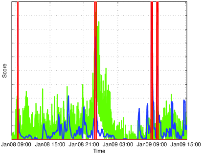
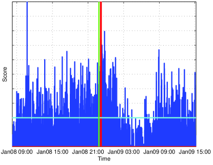
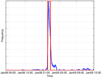
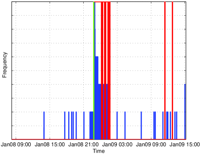
The first alarm time of the proposed link-anomaly-based change-point analysis was 22:55, whereas that for the keyword-frequency-based counterpart was 22:57; see also Table 2. The earliest detection was achieved by the keyword-frequency-based burst detection method. Nevertheless, from Figure 3, we can observe that the proposed link-anomaly-based methods were able to detect the emerging topic almost as early as keyword-frequency-based methods.

Table 2: Detection time and the number of detections. The first detection time is defined as the time of the first alert after the event/post that initiated each topic; see captions for Figures 3–6 for the details.

Method		“Job hunting”	“Youtube”	“NASA”	“BBC”
Link-anomaly-based	$\sharp$ of detections	4	4	14	3
change-point detection	1st detection time	22:55, Jan 08	08:44, Nov 05	20:11, Dec 02	19:52, Jan 21
Keyword-frequency-based	$\sharp$ of detections	1	1	1	1
change-point detection	1st detection time	22:57, Jan 08	00:30, Nov 05	04:10, Dec 03	22:41, Jan 21
Link-anomaly-based	$\sharp$ of detections	1	9	25	2
burst detection	1st detection time	23:07, Jan 08	00:07, Nov 05	00:44, Nov 30	20:51, Jan 21
Keyword-frequency-based	$\sharp$ of detections	6	15	11	1
burst detection	1st detection time	22:50, Jan 08	23:59, Nov 04	08:34, Dec 03	22:32, Jan 21

4.3 “Youtube” data set

This data set is related to the recent leakage of some confidential video by the Japan Coastal Guard officer.

The keyword used in the keyword-based methods is “Senkaku.” Figures 4(a) and 4(b) show the results of link-anomaly-based change detection and burst detection, respectively. Figures 4(c) and 4(d) show the results of keyword-frequency based change detection and burst detection, respectively.

(a) Link-anomaly-based change-point analysis. Green: Aggregated anomaly score (8) at $\tau=1$ minute. Blue: Change-point score (9). Red: Alarm time.

(b) Link-anomaly-based burst detection. Blue: Aggregated anomaly score (8) at $\tau=1$ second. Cyan: threshold for the filtering step in Kleinberg’s burst model. Red: Burst state.

(c) Keyword-frequency-based change-point analysis. Blue: Frequency of keyword “Senkaku” per one minute. Red: Alarm time.

(d) Keyword-frequency-based burst detection. Blue: Frequency of keyword “Senkaku” per one second. Red: Burst state (burst or not).

Figure 4: Result of “Youtube” data set. The first post about the video leakage was posted on 23:48, Nov 04 (green lines in (b) and (d)).

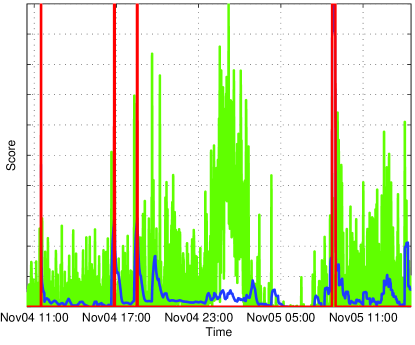
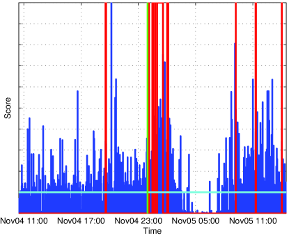
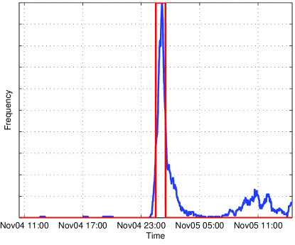
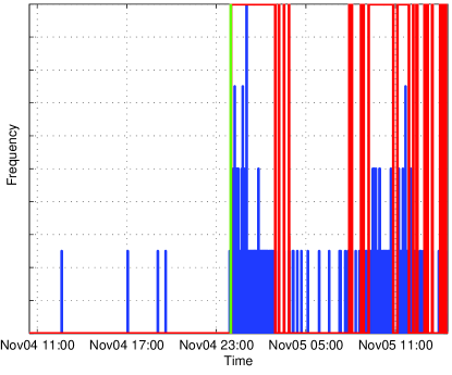
The first alarm time of the proposed link-anomaly-based change-point analysis was 08:44, whereas that for the keyword-based counterpart was 00:30; see also Table 2. Although the aggregated anomaly score (8) in Figure 4(a) around midnight, Nov 05 is elevated, it seems that SDNML fails to detect this elevation as a change point. In fact, the link-anomaly-based burst detection (Figure 4(b)) raised an alarm at 00:07, which is earlier than the keyword-frequency-based change-point analysis and closer to the the keyword-frequency-based burst detection at 23:59, Nov 04.

4.4 “NASA” data set

This data set is related to the discussion among Twitter users interested in astronomy that preceded NASA’s press conference about discovery of an arsenic eating organism.

The keyword used in the keyword-based models is “arsenic.” Figures 5(a) and 5(b) show the results of link-anomaly-based change detection and burst detection, respectively. Figures 5(c) and 5(d) show the same results for the keyword-frequency-based methods.

(a) Link-anomaly-based change-point analysis. Green: Aggregated anomaly score (8) at $\tau=1$ minute. Blue: Change-point score (9). Red: Alarm time.

(b) Link-anomaly-based burst detection. Blue: Aggregated anomaly score (8) at $\tau=1$ second. Cyan: threshold for the filtering step in Kleinberg’s burst model. Red: Burst state.

(c) Keyword-frequency-based change-point analysis. Blue: Frequency of keyword “arsenic” per one minute. Red: Alarm time.

(d) Keyword-frequency-based burst detection. Blue: Frequency of keyword “arsenic” per one second. Red: Burst state (burst or not).

Figure 5: Result of “NASA” data set. The initial post predicting NASA’s finding about arsenic-eating organism was posted on 22:30, Nov 30 much earlier than NASA’s official press conference at 04:00, Dec 03.

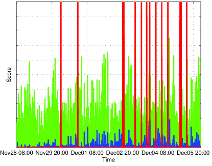
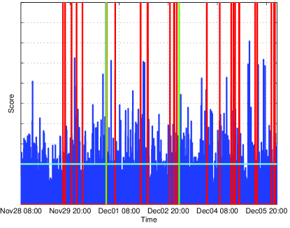
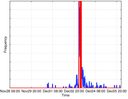
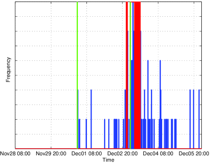
The first alarm times of the two link-anomaly-based methods were 20:11, Dec 02 (change-point detection) and 00:44, Nov 30 (burst detection), respectively. Both of these are earlier than NASA’s official press conference (04:00, Dec 03) and are earlier than the keyword-frequency based methods (change-point detection at 04:10, Dec 03 and burst detection at 08:34, Dec 03.); see Table 2.

4.5 ”BBC” data set

This data set is related to angry reactions among Japanese Twitter users against a BBC comedy show that asked “who is the unluckiest person in the world” (the answer is a Japanese man who got hit by nuclear bombs in both Hiroshima and Nagasaki but survived).

The keyword used in the keyword-based models is “British” (or “Britain”). Figures 6(a) and 6(b) show the results of link-anomaly-based change detection and burst detection, respectively. Figures 6(c) and 6(d) show the same results for the keyword-frequency-based methods.

(a) Link-anomaly-based change-point analysis. Green: Aggregated anomaly score (8) at $\tau=1$ minute. Blue: Change-point score (9). Red: Alarm time.

(b) Link-anomaly-based burst detection. Blue: Aggregated anomaly score (8) at $\tau=1$ second. Cyan: threshold for the filtering step in Kleinberg’s burst model. Red: Burst state.

(c) Keyword-frequency-based change-point analysis. Blue: Frequency of keyword “British” per one minute. Red: Alarm time.

(d) Keyword-frequency-based burst detection. Blue: Frequency of keyword “British” per one second. Red: Burst state (burst or not).

Figure 6: Result of “BBC” data set. The first post about BBC’s comedy show was posted on 17:08, Jan 21 (green lines in (b) and (d)).

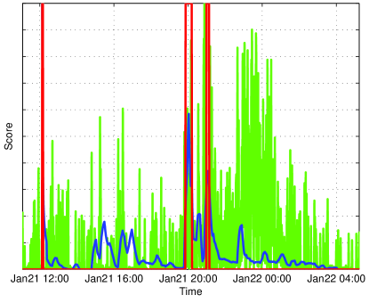
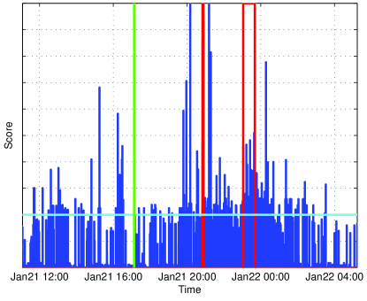
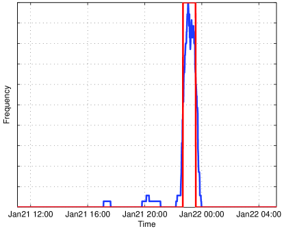
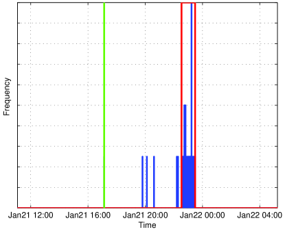
The first alarm time of the two link-anomaly-based methods was 19:52 (change-point detection) and 20:51 (burst detection), both of which are earlier than the keyword-frequency-based counterparts at 22:41 (change-point detection) and 22:32 (burst detection). See Table 2.

4.6 Discussion

Within the four data sets we have analyzed above, the proposed link-anomaly based methods compared favorably against the keyword-frequency based methods on “NASA” and “BBC” data sets. On the other hand, the keyword-frequency based methods were earlier to detect the topics on “Job hunting” and “Youtube” data sets.

The above observation is natural, because for “Job hunting” and “Youtube” data sets, the keywords seemed to have been unambiguously defined from the beginning of the emergence of the topics, whereas for “NASA” and “BBC” data sets, the keywords are more ambiguous. In particular, in the case of “NASA” data set, people had been mentioning “arsenic” eating organism earlier than NASA’s official release but only rarely (see Figure 5(d)). Thus, the keyword-frequency-based methods could not detect the keyword as an emerging topic, although the keyword “arsenic” appeared earlier than the official release. For “BBC” data set, the proposed link-anomaly-based burst model detects two bursty areas (Figure 6(b)). Interestingly, the link-anomaly-based change-point analysis only finds the first area (Figure 6(a)), whereas the keyword-frequency-based methods only find the second area (Figures 6(c) and 6(d)). This is probably because there was an initial stage where people reacted individually using different words and later there was another stage in which the keywords are more unified.

In our approach, the alarm was raised if the change-point score exceeded a dynamically optimized threshold based on the significance level parameter $\rho$. Table 3 shows results for a number of threshold parameter values. We see that as $\rho$ increased, the number of false alarms also increased. Meanwhile, even when it was so small, our approach was still able to detect the emerging topics as early as the keyword-based methods. We set $\rho=0.05$ as a default parameter value in our experiment. Although there are several alarms for “NASA” data set, most of them are more or less related to the emerging topic.

Table 3: Number of alarms for the proposed change-point detection method based on the link-anomaly score (8) for various significance level parameter values $\rho$.

$\rho$	“Job hunting”	“Youtube”	“NASA”	“BBC”
0.01	4	2	9	3
0.05	4	4	14	3
0.1	8	6	30	3

Notice again that in the keyword-based methods the keyword related to the topic must be known in advance, which is not always the case in practice. Further note that our approach only uses links (mentions), hence it can be applied to the case where topics are concerned with information other than texts, such as images, video, sounds, etc.

5 Conclusion

In this paper, we have proposed a new approach to detect the emergence of topics in a social network stream. The basic idea of our approach is to focus on the social aspect of the posts reflected in the mentioning behaviour of users instead of the textual contents. We have proposed a probability model that captures both the number of mentions per post and the frequency of mentionee. We have combined the proposed mention model with the SDNML change-point detection algorithm [3] and Kleinberg’s burst detection model [2] to pin-point the emergence of a topic.

We have applied the proposed approach to four real data sets we have collected from Twitter. The four data sets included a wide-spread discussion about a controversial topic (“Job hunting” data set), a quick propagation of news about a video leaked on Youtube (“Youtube” data set), a rumor about the upcoming press conference by NASA (“NASA” data set), and an angry response to a foreign TV show (“BBC” data set). In all the data sets our proposed approach showed promising performance. In most data set, the detection by the proposed approach was as early as term-frequency based approaches in the hindsight of the keyword that best describes the topic that we have manually chosen afterwards. Furthermore, for “NASA” and “BBC” data sets, in which the keyword that defines the topic is more ambiguous than the first two data sets, the proposed link-anomaly based approaches have detected the emergence of the topics much earlier than the keyword-based approaches.

All the analysis presented in this paper was conducted off-line but the framework itself can be applied on-line. We are planning to scale up the proposed approach to handle social streams in real time. It would also be interesting to combine the proposed link-anomaly model with content-based topic detection approaches to further boost the performance and reduce false alarms.

Appendix A Sequentially discounting normalized maximum likelihood coding

This section describes the sequentially discounting normalized maximum likelihood (SDNML) coding that we use for change-point detection in Section 3.4. The basic idea behind SDNML-based change detection is as follows: when the data arrives in a sequential manner, we can consider a change has occurred if a new piece of data cannot be compressed using the statistical nature of the past. The original paper [10, 11] used the predictive stochastic complexity as a measure of compressibility, whereas Urabe et al. [3] proposed to employ a tighter coding scheme based on the SDNML.

Suppose that we observe a discrete time series $x_{t}$ ($t=1,2,\ldots,$); we denote the data sequence by $x^{t}:=x_{1}\cdots x_{t}$. Consider the parametric class of conditional probability densities $\mathcal{F}=\{p(x_{t}|x^{t-1}:\boldsymbol{\theta}):\boldsymbol{\theta}\in\mathbf{R}^{p}\}$, where $\boldsymbol{\theta}$ is the $p$-dimensional parameter vector and we assume $x^{0}$ to be an empty set. We denote the maximum likelihood (ML) estimator given the data sequence $x^{t}$ by $\hat{\boldsymbol{\theta}}(x^{t})$; i.e., $\hat{\boldsymbol{\theta}}(x^{t}):={\rm argmax}_{\boldsymbol{\theta}\in\mathbf{R}^{p}}\prod_{j=1}^{t}p(x_{j}|x^{j-1}:\boldsymbol{\theta})$. The sequential normalized maximum likelihood (SNML) model is a coding distribution (see e.g., [15]) that is known to be optimal in the sense of the conditional minimax [16] problem:

$$\min_{q(\cdot|x^{t-1})}\max_{x_{t}}\left(-\log q(x_{t}|x^{t-1})+\max_{\boldsymbol{\theta}\in\mathbf{R}^{p}}\log p(x^{t}:\boldsymbol{\theta})\right),$$ (10)

where $p(x^{t}):=\prod_{j=1}^{t}p(x_{j}|x^{j-1}:\boldsymbol{\theta})$ is the joint density over $x^{t}$ induced by the conditional densities from $\mathcal{F}$. The minimization is taken over all conditional density functions and tries to minimize the regret (10) over any possible outcome of the new sample $x_{t}$.

The SNML distribution is obtained as the optimal conditional density of the minimax problem (10) as follows [16]:

$$p_{\mbox{\tiny SNML}}(x_{t}|x^{t-1}):=\frac{p(x^{t}:\hat{\boldsymbol{\theta}}(x^{t}))}{K_{t}(x^{t-1})},$$ (11)

where the normalization constant $K_{t}(x^{t-1}):=\int p(x^{t}|\hat{\boldsymbol{\theta}}(x^{t})){\rm d}x_{t}$ is necessary because the new sample $x_{t}$ is used in the estimation of parameter vector $\hat{\boldsymbol{\theta}}(x^{t})$ and the numerator in (11) is not a proper density function. We call the quantity $-\log p_{\mbox{\tiny SNML}}(x_{t}|x^{t-1})$ the SNML code-length. It is known from [16, 13] that the cumulative SNML code-length, which is the sum of SNML code-length over the sequence, is optimal in the sense that it asymptotically achieves the shortest code-length.

The sequentially discounting normalized maximum likelihood (SDNML) is obtained by applying the above SNML to the class of autoregressive (AR) model and replacing the ML estimation in (11) with a discounted ML estimation, which makes the SDNML-based change-point detection algorithm more flexible than an SNML-based one. Let $x_{t}\in\mathbf{R}$ for each $t$. We define the $p$th order AR model as follows:

$$p(x_{t}|x_{t-k}^{t-1}:\boldsymbol{\theta})=\frac{1}{\sqrt{2\pi\sigma^{2}}}\exp\Biggl{(}-\frac{1}{2\sigma^{2}}\Bigl{(}x_{t}-\sum_{i=1}^{p}a^{(i)}x_{t-i}\Bigr{)}^{2}\Biggr{)},$$

where $\boldsymbol{\theta}^{\top}=(\boldsymbol{a}^{\top},\sigma^{2})=((a^{(1)},\ldots,a^{(p)}),\sigma^{2})$ is the parameter vector.

In order to compute the SDNML density function we need the discounted ML estimators of the parameters in $\boldsymbol{\theta}$. We define the discounted ML estimator of the regression coefficient $\hat{\boldsymbol{a}}_{t}$ as follows:

$$\hat{\boldsymbol{a}}_{t} =\mathop{\rm argmin}_{\boldsymbol{a}\in\mathbf{R}^{p}}\sum_{j=t_{0}+1}^{t}w_{t-j}\left(x_{j}-\boldsymbol{a}^{\top}\bar{\boldsymbol{x}}_{j}\right)^{2},$$ (12)

where $w_{j^{\prime}}=r(1-r)^{j^{\prime}}$ is a sequence of sample weights with the discounting coefficient $r$ ($0<r<1$); $t_{0}$ is the smallest number of samples such that the minimizer (12) is unique; $\bar{\boldsymbol{x}}_{j}:=(x_{j-1},x_{j-2},\ldots,x_{j-k})^{\top}$. Note that the error terms from older samples receive geometrically decreasing weights in (12). The larger the discounting coefficient $r$ is, the smaller the weights of the older samples become; thus we have stronger discounting effect. Moreover, we obtain the discounted ML estimator of the variance $\hat{\tau}_{t}$ as follows:

$$\hat{\tau}_{t}:= \mathop{\rm argmax}_{\sigma^{2}}\prod_{j=t_{0}+1}^{t}p\left(x_{j}|x_{j-k}^{j-1}:\hat{\boldsymbol{a}}_{j},\sigma^{2}\right)$$

$$= \frac{1}{t-t_{0}}\sum_{j=t_{0}+1}^{t}\hat{e}_{j}^{2}=\frac{S_{t}}{t-t_{0}},$$

where we define $\hat{e}_{j}^{2}=\left(x_{j}-\hat{\boldsymbol{a}}_{j}^{\top}\bar{\boldsymbol{x}}_{j}\right)^{2}$ and $S_{t}:=\sum_{j=t_{0}+1}^{t}\hat{e}_{j}^{2}$. Clearly when the discounted estimator of the AR coefficient $\hat{\boldsymbol{a}}_{j}$ is available, $S_{t}$ can be computed in a sequential manner.

In the sequel, we first describe how to efficiently compute the AR estimator $\hat{\boldsymbol{a}}_{j}$. Finally we derive the SDNML density function using the discounted ML estimators $(\hat{\boldsymbol{a}}_{t},\hat{\tau}_{t})$.

The AR coefficient $\hat{\boldsymbol{a}}_{j}$ can simply be computed by solving the least-squares problem (12). It can, however, be obtained more efficiently using the iterative formula described in [16, 13]. Here we repeat the formula for the discounted version presented in [3]. First define the sufficient statistics $V_{t}\in\mathbf{R}^{p\times p}$ and $\boldsymbol{\chi}_{t}\in\mathbf{R}^{p}$ as follows:

$$V_{t}:=\sum_{j=t_{0}+1}^{t}w_{j}\bar{\boldsymbol{x}}_{j}\bar{\boldsymbol{x}}_{j}^{\top},\quad\boldsymbol{\chi}_{t}:=\sum_{j=t_{0}+1}^{t}w_{j}\bar{\boldsymbol{x}}_{j}x_{j}.$$

Using the sufficient statistics, the discounted AR coefficient $\hat{\boldsymbol{a}}_{j}$ from (12) can be written as follows:

$$\hat{\boldsymbol{a}}_{t} =V_{t}^{-1}\boldsymbol{\chi}_{t}.$$

Note that $\boldsymbol{\chi}_{t}$ can be computed in a sequential manner. The inverse matrix $V_{t}^{-1}$ can also be computed sequentially using the Sherman-Morrison-Woodbury formula as follows:

$$V_{t}^{-1} =\frac{1}{1-r}V_{t}^{-1}-\frac{r}{1-r}\frac{V_{t}^{-1}\bar{\boldsymbol{x}}_{t}\bar{\boldsymbol{x}}_{t}^{\top}V_{t}^{-1}}{1-r+c_{t}},$$

where $c_{t}=r\bar{\boldsymbol{x}}_{t}^{\top}V_{t}^{-1}\bar{\boldsymbol{x}}_{t}$.

Finally the SDNML density function is written as follows:

$$p_{\mbox{\tiny SDNML}}(x_{t}|x^{t-1}) =\frac{1}{K_{t}(x^{t-1})}\frac{s_{t}^{-(t-t_{0})/2}}{s_{t-1}^{-(t-t_{0}-1)/2}},$$

where the normalization factor $K_{t}(x^{t-1})$ is calculated as follows:

$$K_{t}(x^{t-1}) =\frac{\sqrt{\pi}}{1-d_{t}}\sqrt{\frac{1-r}{r}}(1-r)^{-\frac{t-m}{2}}\frac{\Gamma((t-t_{0}-1)/2)}{\Gamma((t-t_{0})/2)},$$

with $d_{t}=c_{t}/(1-r+c_{t})$.

References

- [1] J. Allan, J. Carbonell, G. Doddington, J. Yamron, Y. Yang et al., “Topic detection and tracking pilot study: Final report,” in Proceedings of the DARPA broadcast news transcription and understanding workshop, 1998.
- [2] J. Kleinberg, “Bursty and hierarchical structure in streams,” Data Min. Knowl. Disc., vol. 7, no. 4, pp. 373–397, 2003.
- [3] Y. Urabe, K. Yamanishi, R. Tomioka, and H. Iwai, “Real-time change-point detection using sequentially discounting normalized maximum likelihood coding,” in Proceedings. of the 15th PAKDD, 2011.
- [4] S. Morinaga and K. Yamanishi, “Tracking dynamics of topic trends using a finite mixture model,” in Proceedings of the 10th ACM SIGKDD, 2004, pp. 811–816.
- [5] Q. Mei and C. Zhai, “Discovering evolutionary theme patterns from text: an exploration of temporal text mining,” in Proceedings of the 11th ACM SIGKDD, 2005, pp. 198–207.
- [6] A. Krause, J. Leskovec, and C. Guestrin, “Data association for topic intensity tracking,” in Proceedings of the 23rd ICML, 2006, pp. 497–504.
- [7] D. He and D. S. Parker, “Topic dynamics: an alternative model of bursts in streams of topics,” in Proceedings of the 16th ACM SIGKDD, 2010, pp. 443–452.
- [8] H. Small, “Visualizing science by citation mapping,” Journal of the American society for Information Science, vol. 50, no. 9, pp. 799–813, 1999.
- [9] D. Aldous, “Exchangeability and related topics,” in École d’Été de Probabilités de Saint-Flour XIII—1983. Springer, 1985, pp. 1–198.
- [10] K. Yamanishi and J. Takeuchi, “A unifying framework for detecting outliers and change points from non-stationary time series data,” in Proceedings of the 8th ACM SIGKDD, 2002.
- [11] J. Takeuchi and K. Yamanishi, “A unifying framework for detecting outliers and change points from time series,” IEEE T. Knowl. Data En., vol. 18, no. 44, pp. 482–492, 2006.
- [12] J. Rissanen, “Strong optimality of the normalized ML models as universal codes and information in data,” IEEE T. Inform. Theory, vol. 47, no. 5, pp. 1712–1717, 2002.
- [13] J. Rissanen, T. Roos, and P. Myllymäki, “Model selection by sequentially normalized least squares,” Journal of Multivariate Analysis, vol. 101, no. 4, pp. 839–849, 2010.
- [14] K. Yamanishi and Y. Maruyama, “Dynamic syslog mining for network failure monitoring,” Proceeding of the 11th ACM SIGKDD, p. 499, 2005.
- [15] T. M. Cover and J. A. Thomas, Elements of Information Theory. New York: Wiley & Sons, 1991, 2nd edition, 2006.
- [16] T. Roos and J. Rissanen, “On sequentially normalized maximum likelihood models,” in Workshop on information theoretic methods in science and engineering, 2008.