H-Matrix and Block Error Tolerances

Abstract

We describe a new method to map the requested error tolerance on an H-matrix approximation to the block error tolerances. Numerical experiments show that the method produces more efficient approximations than the standard method for kernels having singularity order greater than one, often by factors of $1.5$ to $5$ and at a lower computational cost.

1 Introduction

A completely dense matrix $B$ arising from an integral or sum involving a singular kernel over a surface or particles can be approximated efficiently by a hierarchical matrix, called an H-matrix (hlib, ). Let $\bar{B}$ be the H-matrix approximation to $B$.

Let the surface be discretized by $N$ elements or let there be $N$ particles. The two cases differ essentially only in how a matrix entry of $B$ is calculated. If $B$ includes all and only pair-wise interactions, then $B\in\mathbb{R}^{N\times N}$. In this paper $B$ is always square, but the results extend to the rectangle case $B\in\mathbb{R}^{M\times N}$ by replacing occurrences of $N^{2}$ by $MN$. The procedure to construct an H-matrix has four parts. First, a cluster tree over the particles is formed. The cluster tree induces a (nonunique) symmetric permutation of $B$. For notational brevity, hereafter we assume $B$ is already ordered such that the identity matrix is a permutation matrix induced by the cluster tree. Second, pairs of clusters are found that satisfy certain criteria; associated with such a pair is a block of $B$. Third, the requested error tolerance $\varepsilon$ (hereafter usually just tolerance) is mapped to block tolerances. A tolerance specifies the maximum error allowed. Fourth, each block is approximated by a low-rank approximation (LRA) that satisfies that block’s tolerance. A number of LRA algorithms are available.

An LRA to a block $B_{i}$ can be efficiently expressed as an outer product of two matrices $U$ and $V$: $B_{i}\approx\bar{B}_{i}=UV^{T}$. Let $r$ be the number of columns in $U$; then $r$ is the maximum rank of $\bar{B}_{i}$ and the rank if $U$ and $V$ have independent columns, as is always the case in this context. Let $\text{nnz}(B_{i})$ be the number of nonzero numbers required to represent $B_{i}$ exactly, and similarly for other matrices. Hence $\text{nnz}(B)=N^{2}$; if $B_{i}\in\mathbb{R}^{m\times n}$, then $\text{nnz}(B_{i})=mn$ and $\text{nnz}(\bar{B}_{i})=\text{nnz}(U)+\text{nnz}(V)=(m+n)r$; and if $\bar{B}$ is partitioned according to the index set ${\cal I}$, then $\text{nnz}(\bar{B})=\sum_{i\in{\cal I}}\text{nnz}(\bar{B}_{i})$. The efficiency of an H-matrix approximation $\bar{B}$ is measured by its compression, $\text{nnz}(B)/\text{nnz}(\bar{B})=N^{2}/\text{nnz}(\bar{B})$. A standard application of an H-matrix approximation is to a sequence of matrix-vector products (MVP) with dense vectors. The work to compute an MVP is proportional to $\text{nnz}(\bar{B})$.

In this paper we focus on the third part of constructing an H-matrix: how to map the requested tolerance $\varepsilon$ on $\bar{B}$ to block tolerances. An efficient method has at least these three properties. First, the tolerance is met. Second, the tolerance is not exceeded by much: any unrequested additional accuracy reduces the compression. Third, the method must not add much work to the construction process relative to a standard method; indeed, if the resulting compression is greater, the work will likely be less. We propose a method based on the inequality (7) that has these properties.

It may be worth emphasizing the importance of an algorithm’s meeting a tolerance without exceeding it by much. Many computational mathematical algorithms trade between speed and accuracy. A tolerance has two roles: first, it is the means by which the user controls the tradeoff; second, the associated error bound, either by itself or in combination with those from other algorithms in a larger framework, gives the accuracy of the approximate solution to the problem. A user who detects that an algorithm is giving much greater accuracy than requested is tempted to request less accuracy. Such a procedure requires more work in the form of repeated solutions of trial problems until the speed-accuracy tradeoff appears—but cannot be known with certainty—to be satisfactory; and it sacrifices an assured error bound because the relationship between tolerance and error bound is not clear. The method we shall describe does not principally increase compression, relative to the standard method, for a given (unknown) achieved error (though it does in important cases in our experiments); rather, it increases compression for a given requested error tolerance by achieving an error that is not much less than the tolerance.

2 The meaning of the requested error tolerance

In this paper and as often implemented in H-matrix software, the tolerance $\varepsilon$ specifies the maximum allowed Frobenius-norm-wise relative error of the approximation $\bar{B}$ to $B$. Let $E\equiv B-\bar{B}$. It is requested that $\bar{B}$ satisfy

$$\|E\|_{\text{F}}\leq\varepsilon\|B\|_{\text{F}}\quad\text{or, equivalently,}\quad\frac{\|B-\bar{B}\|_{\text{F}}}{\|B\|_{\text{F}}}\leq\varepsilon.$$ (1)

If (1) holds, then $\|Ex\|_{\text{F}}\leq\|E\|_{\text{F}}\|x\|_{2}\leq\varepsilon\|B\|_{\text{F}}\|x\|_{2}$. Rearranging, the relative error in an MVP is bounded as

$$\frac{\|Bx-\bar{B}x\|_{2}}{\|B\|_{\text{F}}\|x\|_{2}}\leq\varepsilon.$$ (2)

If $B$ is square and nonsingular (as it is in this application), then we can obtain a simple expression for the maximum perturbation to $x$ that yields the same error as $\bar{B}$ makes. Let $y=Bx$. Let $\bar{y}\equiv\bar{B}x$; we want to bound $\|\delta x\|_{2}$ such that $\bar{y}=B(x+\delta x)$. Rearranging, $\delta x=B^{-1}(\bar{y}-Bx)=B^{-1}(\bar{y}-y)$. By (2), $\|\bar{y}-y\|_{2}\leq\varepsilon\|B\|_{\text{F}}\|x\|_{2}$ and so $\|\delta x\|_{2}\leq\varepsilon\|B^{-1}\|_{\text{F}}\|B\|_{\text{F}}\|x\|_{2}$, or

$$\frac{\|\delta x\|_{2}}{\|x\|_{2}}\leq\varepsilon\kappa_{\text{F}}(B),$$ (3)

where $\kappa_{\text{F}}(B)$ is the condition number of $B$ in the Frobenius norm. If (1) instead has the form $\|E\|_{\text{F}}\leq\varepsilon\|B\|_{2}$, then ‘2’ replaces ‘F’ in (2) and (3).

One can also specify an element-wise error (EWE) of the approximation $\bar{B}$ to $B$. Let $\max_{i,j}|E_{i,j}|\equiv\|E\|_{\text{max}}$: this is the element-wise max-norm. In this case, it is requested that $\bar{B}$ satisfy

$$\|E\|_{\text{max}}\leq\varepsilon N^{-1}\|B\|_{1}\equiv\bar{\varepsilon}.$$ (4)

If (4) holds, then $\|Ex\|_{1}\leq\bar{\varepsilon}\|x\|_{1}\|e\|_{1}=\bar{\varepsilon}\|x\|_{1}N=\varepsilon\|B\|_{1}\|x\|_{1}$, where $e$ is the vector of all ones, and so the relative error in an MVP is bounded as

$$\frac{\|Bx-\bar{B}x\|_{1}}{\|B\|_{1}\|x\|_{1}}\leq\varepsilon,$$

which is the same as (2) except the 1-norm is used. Similarly, one obtains the analogue of (3):

$$\frac{\|\delta x\|_{1}}{\|x\|_{1}}\leq\varepsilon\kappa_{1}(B).$$

Observe that an element-wise norm (Frobenius, max) applied to blocks yields an error bound in $p$-norms (respectively 2 and 1).

3 Meeting the requested error tolerance

Let a matrix be partitioned into blocks indexed by $i\in{\cal I}$; we often write $\sum_{i}$ rather than $\sum_{i\in{\cal I}}$. We need to satisfy the bound (1) on the whole matrix based on information in each block. The bound may be achieved by at least three methods.

The first method—really, a class of methods—is to prescribe the rank of each block based on analysis of problem-specific information: for example, an integral equation and its discretization (panel-cluster, ); or in the context of proving error bounds for far more sophisticated hierarchical algorithms than we consider: for example, the H²-matrix method of borm-h2-variable . Our interest is in applying the relatively simple H-matrix method to arbitrary kernels, and so we do not further consider these approaches.

We call the second method the block-wise relative-error method (BREM). This method is standard in practice: for example, equation (3.69) and surrounding text in bebendorf_book , the software package AHMED by the same author, numerical experiments in Chapter 4 of rjasanow-book , and relevant experiments in Section 4.8 of hlib all use or describe this method. Each LRA $\bar{B}_{i}$ to block $B_{i}$ is computed to satisfy

$$\|E_{i}\|_{\text{F}}\leq\varepsilon\|B_{i}\|_{\text{F}}.$$ (5)

Then

$$\|E\|_{\text{F}}^{2}=\sum_{i}\|E_{i}\|_{\text{F}}^{2}\leq\varepsilon^{2}\sum_{i}\|B_{i}\|_{\text{F}}^{2}=\varepsilon^{2}\|B\|_{\text{F}}^{2},$$ (6)

which implies (1).

The third method supposes $\|B\|_{\text{F}}$ is known. We call it the matrix-wise relative-error method (MREM). We believe that this method, though simple, is new. Each LRA $\bar{B}_{i}$ to $B_{i}\in\mathbb{R}^{m_{i}\times n_{i}}$ is computed to satisfy

$$\|E_{i}\|_{\text{F}}\leq\varepsilon\frac{\sqrt{m_{i}n_{i}}}{N}\|B\|_{\text{F}}.$$ (7)

As $N^{2}=\sum_{i\in{\cal I}}m_{i}n_{i}$,

$$\|E\|_{\text{F}}^{2}=\sum_{i}\|E_{i}\|_{\text{F}}^{2}\leq\varepsilon^{2}N^{-2}\|B\|_{\text{F}}^{2}\sum_{i}m_{i}n_{i}=\varepsilon^{2}\|B\|_{\text{F}}^{2},$$ (8)

which again implies (1).

If (5) and (7) are equalities rather than inequalities, then so are respectively (6) and (8).

The efficiencies of BREM and MREM are determined by the magnitudes $\|B_{i}\|_{\text{F}}$ and $N^{-1}\sqrt{m_{i}n_{i}}\|B\|_{\text{F}}$, respectively, as a function of $i\in{\cal I}$. One magnitude cannot dominate the other for all $i\in{\cal I}$: as equality is possible in (6) and (8), if for one block the first magnitude is greater than the other, then there is at least one other block for which the opposite holds.

MREM requires that a block LRA satisfy (on rearranging (7))

$$(m_{i}n_{i})^{-1}\|E_{i}\|_{\text{F}}^{2}\leq\varepsilon N^{-2}\|B\|_{\text{F}}^{2}.$$ (9)

On each side of this inequality—omitting $\varepsilon$ on the right side—is a quantity we call the Frobenius norm squared per element (FNPE). If we also square and divide (5) by $m_{i}n_{i}$, then our two magnitudes from before become respectively the block and matrix FNPE $(m_{i}n_{i})^{-1}\|B_{i}\|_{\text{F}}^{2}$ and $N^{-2}\|B\|_{\text{F}}^{2}$. For a matrix $B$ arising from a singular kernel, the block FNPE is smaller for far-off-diagonal blocks than for near- and on-diagonal blocks. Hence relative to BREM, MREM requests less accuracy for far-off-diagonal blocks and more for the others.

BREM and MREM require different termination criteria in the block LRA algorithm. BREM requires the LRA algorithm to terminate based on an estimate of the relative error with tolerance $\varepsilon$; MREM, the absolute error with tolerance $\varepsilon N^{-1}\sqrt{m_{i}n_{i}}\|B\|_{\text{F}}$. Neither termination criterion is more difficult to implement, or requires more work to evaluate (within a small number of operations), than the other.

So far we have discussed the error bound in the Frobenius norm; now we discuss the bound in the max-norm. If every block $i$ satisfies

$$\|E_{i}\|_{\text{max}}\leq\bar{\varepsilon},$$ (10)

then (4) holds. We call this procedure MREMmax. Consider the inequalities (9) and (10). In both, the right side is an absolute tolerance that is the same for every block; and the left side describes an element-wise quantity: in the first, the FNPE; in the second, the maximum magnitude. Hence MREM and MREMmax behave similarly in how they map the matrix tolerance to the block ones. It is not clear to us whether there are any applications that use MREMmax rather than BREM. We shall shortly discuss why MREM is preferable to MREMmax in practice.

3.1 Estimating $\|B\|_{\text{F}}$

In some problems $\|B\|_{\text{F}}$ may be available, but we also need a means to estimate this norm. We describe two methods.

The first is a stochastic method. Let $\{X_{i}\}$ be $n$ iid samples. The estimator of the mean is, as usual, $\mu\equiv n^{-1}\sum_{i}X_{i}$. It is useful to estimate confidence intervals on the estimator $\mu$ using a resampling method. A straightforward approach is to compute the delete-1 jackknife variance of the estimator, which in this simple case is $n^{-1}\sum_{i}(X_{i}-\mu)^{2}$. We use the square root of this value and call it the jackknife standard deviation (JSD).

To estimate $\|B\|_{\text{F}}^{2}$, we could select a subset of entries. In practice we choose to select a random subset of columns. This choice implies $X_{i}\equiv N\sum_{j=1}^{N}B_{ji}^{2}$. We increase the number of columns until the JSD is less than a requested tolerance.

A second method is to obtain an initial approximation $\tilde{B}$ to $B$ with a very large tolerance $\tilde{\varepsilon}$. One can use either BREM or MREM; if MREM, use the stochastic method to obtain the initial estimate of $\|B\|_{\text{F}}$. As $\|B-\tilde{B}\|_{\text{F}}\leq\tilde{\varepsilon}\|B\|_{\text{F}}$ and $\tilde{B}=B+(\tilde{B}-B)$, $\|\tilde{B}\|_{\text{F}}\leq(1+\tilde{\varepsilon})\|B\|_{\text{F}}$. Hence we can safely use $(1+\tilde{\varepsilon})^{-1}\|\tilde{B}\|_{\text{F}}$ as the estimate of $\|B\|_{\text{F}}$ in MREM to obtain the final approximation $\bar{B}$. Computing $\|\tilde{B}\|_{\text{F}}$ requires work proportional to $\text{nnz}(\tilde{B})$.

3.2 Recompression

Let $B\in\mathbb{R}^{m\times n}$ now be a block; in this subsection we suppress the subscript $i$. Let $\bar{B}^{1}=U^{1}(V^{1})^{T}$ be the rank-$r$ output of an LRA algorithm. One can improve a suboptimal LRA by using a recompression algorithm (bebendorf_book, ). Such an algorithm attempts to compress $\bar{B}^{1}$; the algorithm’s efficiency results from the outer-product structure of $\bar{B}^{1}$ and that $B$ is not accessed at all. For the latter reason, the algorithm’s error bound must be based on only $\bar{B}^{1}$. An example of a recompression algorithm is to compute the singular value decomposition (SVD) of $\bar{B}^{1}$—which is efficient because of the outer-product structure of $\bar{B}^{1}$—and then to discard some subset of the singular values and vectors. Let $\bar{B}^{2}$ be the output of a recompression algorithm.

Let $\varepsilon$ be a block absolute tolerance, as in MREM and MREMmax. We must assure $\|B-\bar{B}^{2}\|_{\text{F}}\leq\varepsilon$; what follows also holds if ‘F’ is replaced by ‘max’. Let $0<\alpha<1$. First, compute $\bar{B}^{1}$ so that $\|B-\bar{B}^{1}\|_{\text{F}}\leq\alpha\varepsilon$. Second, compute $\bar{B}^{2}$ so that $\|\bar{B}^{1}-\bar{B}^{2}\|_{\text{F}}\leq(1-\alpha)\varepsilon$; for generality later, let $\beta\equiv 1-\alpha$. As $B-\bar{B}^{2}=(B-\bar{B}^{1})+(\bar{B}^{1}-\bar{B}^{2})$, $\|B-\bar{B}^{2}\|_{\text{F}}\leq\|B-\bar{B}^{1}\|_{\text{F}}+\|\bar{B}^{1}-\bar{B}^{2}\|_{\text{F}}\leq\alpha\varepsilon+(1-\alpha)\varepsilon=\varepsilon$, and so $\bar{B}^{2}$ satisfies the tolerance.

Now let $\varepsilon$ be a block relative tolerance, as in BREM. We must assure $\|B-\bar{B}^{2}\|_{\text{F}}\leq\varepsilon\|B\|_{\text{F}}$. Again, let $0<\alpha<1$; we must determine $\beta>0$. First, compute $\bar{B}^{1}$ so that $\|B-\bar{B}^{1}\|_{\text{F}}\leq\alpha\varepsilon\|B\|_{\text{F}}$. Second, compute $\bar{B}^{2}$ so that $\|\bar{B}^{1}-\bar{B}^{2}\|_{\text{F}}\leq\beta\varepsilon\|\bar{B}^{1}\|_{\text{F}}$. If in this second inequality the right side involved $\|B\|_{\text{F}}$ rather than $\|\bar{B}^{1}\|_{\text{F}}$, then the calculation would be the same as in the case of absolute error. But here we must bound $\|\bar{B}^{1}\|_{\text{F}}$. As $\bar{B}^{1}=(\bar{B}^{1}-B)+B$, $\|\bar{B}^{1}\|_{\text{F}}\leq\|B-\bar{B}^{1}\|_{\text{F}}+\|B\|_{\text{F}}$. From the first step, $\|B-\bar{B}^{1}\|_{\text{F}}\leq\alpha\varepsilon\|B\|_{\text{F}}$, and so $\|\bar{B}^{1}\|_{\text{F}}\leq(1+\alpha\varepsilon)\|B\|_{\text{F}}$. Let $\beta=(1-\alpha)/(1+\alpha\varepsilon)$. Then $\|B-\bar{B}^{2}\|_{\text{F}}\leq\|B-\bar{B}^{1}\|_{\text{F}}+\|\bar{B}^{1}-\bar{B}^{2}\|_{\text{F}}\leq\alpha\varepsilon\|B\|_{\text{F}}+\beta\varepsilon\|\bar{B}^{1}\|_{\text{F}}\leq\alpha\varepsilon\|B\|_{\text{F}}+(1-\alpha)\varepsilon\|B\|_{\text{F}}=\varepsilon\|B\|_{\text{F}}$, and so again $\bar{B}^{2}$ satisfies the tolerance.

In the case of SVD recompression, following Section 1.1.4 of bebendorf_book , let $Q_{U}R_{U}$ be the thin QR factorization of $U^{1}$ and similarly for $V^{1}$. Let $W\Sigma Z^{T}$ be the SVD of $R_{U}R_{V}^{T}$. Then $Q_{U}W\Sigma Z^{T}Q_{V}^{T}$ is the thin SVD of $\bar{B}^{1}$. This SVD is obtained with $O((m+n)r^{2}+r^{3})$ work. Choose the first $k\leq r$ columns of $W$ and $V$ and singular values $\sigma_{i}$ and set $U^{2}=Q_{U}W_{\text{:}\text{,}1\text{:}k}\Sigma_{1\text{:}k\text{,}1\text{:}k}$ and $V^{2}=Q_{V}Z_{\text{:}\text{,}1\text{:}k}$. This gives the LRA $\bar{B}^{2}=U^{2}(V^{2})^{T}$; $\text{nnz}(\bar{B}^{2})\leq\text{nnz}(\bar{B}^{1})$, with strict inequality if $k<r$. When one uses MREM and so the Frobenius norm, one chooses $k$ based on the inequality $\|\bar{B}^{2}_{k}-\bar{B}^{1}\|_{\text{F}}\leq\beta\varepsilon$, where $\bar{B}^{2}_{k}$ uses the $k$ largest singular values and associated vectors. Because $\|\bar{B}^{2}_{k}-\bar{B}^{1}\|_{\text{F}}=(\sum_{i=k+1}^{r}\sigma_{i}^{2})^{1/2}$, choosing $k$ requires just $O(r)$ operations. Using MREMmax entails more work because there is no simple relationship between the singular values and the max-norm. One performs a binary search on the ordered list of singular values. At each step, all the elements of $\bar{B}^{2}_{k}$ must be computed and compared with $\bar{B}^{1}$ to find the maximum deviation. Hence selecting $k$ requires $O(mn\log r)$ work; this work can dominate the work to compute the SVD if $r$ is small relative to $m$ and $n$. Because SVD recompression is a very effective way to improve an LRA, MREM is preferable to MREMmax if one does not prefer the 1- to the 2-norm in the associated error bounds.

4 Numerical experiments

We have several goals for our numerical experiments. First, of course, we must show that MREM can yield greater compression than BREM on at least some problems of interest. Second, we want to show that MREM is robust: ideally, it should never yield less compression than BREM. Third, we are interested in the errors that MREM achieves: are they indeed only slightly better than requested?

We use adaptive cross approximation (ACA) (bebendorf-aca, ) as implemented in AHMED to find block LRA. To implement the absolute block tolerance required by MREM, we modified two lines of code. A good LRA algorithm must compress a matrix well while requesting as few matrix entry evaluations as possible. We find that ACA is quite efficient and robust on the problems in our test set. It terminates when the relative error is within a factor of approximately 10 either side of the tolerance; in particular, note carefully that occasionally (but infrequently) the error is worse than requested. Of course ACA could terminate with a more precise error, but increased termination precision would entail additional work. Instead, we accommodate this behavior as follows. Let $\varepsilon$ be the block tolerance. In the recompression tolerance we set $\alpha=1/2$; if MREM is used, $\beta=\alpha$; if BREM, $\beta$ is as described in Section 3.2. We run ACA with a tolerance of $\alpha\varepsilon/10$, where the factor of $1/10$ compensates for ACA’s sometimes imprecise termination behavior, and then the SVD recompression algorithm with $\beta\varepsilon$. LRA algorithms based on interpolation (e.g., hybrid-aca ) mitigate the problem of terminating with less accuracy than requested while still remaining efficient. In any case, the choice of LRA algorithm is independent of the choice of either BREM or MREM.

We estimate $\|B\|_{\text{F}}$ using the stochastic method described in 3.1. The estimator is terminated when the JSD is no greater than $1/50$. To be conservative, we subtract two JSD from the estimate of $\|B\|_{\text{F}}$, thereby effectively decreasing the tolerance slightly.

4.1 Particle distributions

We perform numerical experiments using a distribution of point-like particles that interact according to the kernel $K(r)=1/r^{p}$ if $r>0$, $0$ otherwise, where $r$ is the distance between two points and $p$ is the order of the singularity. We also consider the kernel $K(r)=\ln r$.

We consider singularity orders $p=1$, $2$, $3$ and three geometries: uniform distribution of points in the cube $[-1,1]^{3}$, on its surface, and on its edges; where indicated in figures, these are denoted respectively ‘cube’, ‘surf’, and ‘edge’. The requested error tolerance $\varepsilon$ is usually $10^{-5}$. We measure several quantities. The one that most clearly demonstrates the performance of MREM relative to BREM is the improvement factor (IF), $\text{nnz}(\bar{B}^{\text{B}})/\text{nnz}(\bar{B}^{\text{M}})$, where the superscripts B and M denote BREM and MREM. A value greater than one indicates improvement.

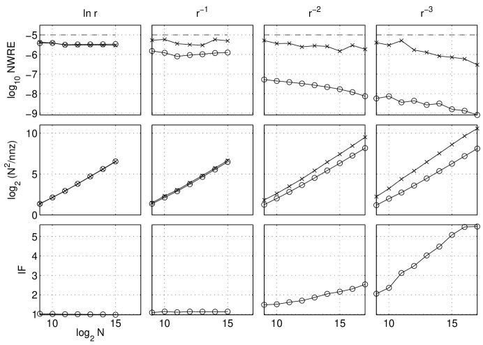
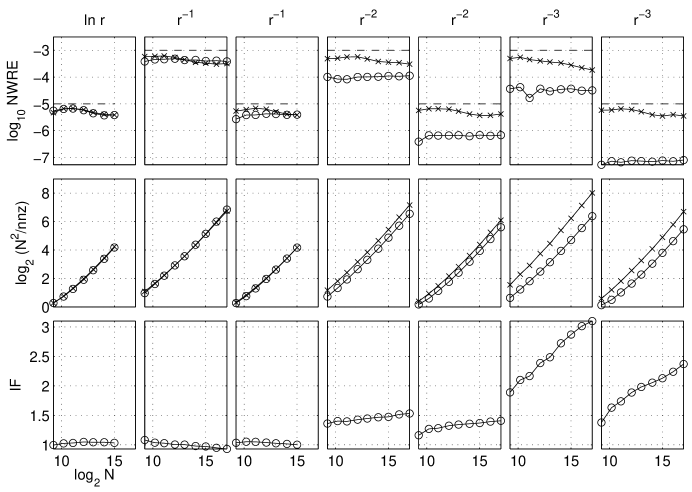
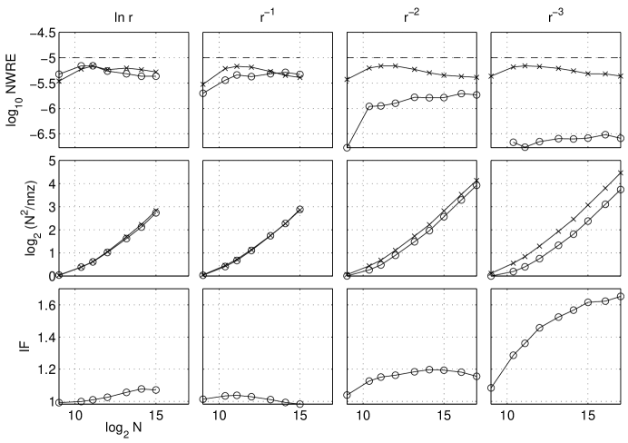
Figures 1, 2, and 3 show results for the three geometries. Each column corresponds to a kernel, which is stated at the top of the column, and tolerance $\varepsilon$, indicated by the dashed horizontal line in the top row. In the top two rows, curves for BREM have circles; for MREM, x’s. All rows plot quantities against problem size $N$. The top row shows the Frobenius-norm-wise relative error achieved; these are estimates for problems having size $N>2^{15}$. The middle row shows the compression factor. The bottom row shows the improvement factor of MREM. Most experiments were carried out to approximately $2^{17}$ particles, though in a few cases the runs were terminated early to save computation time or because of memory size.

Trends accord with our observations in Section 3. The IF increases as the dominance of the (near) diagonal of $B$ increases. In the context of our test problems, the IF increases with increasing order $p$ and sparser geometry. The IF rarely is below 1, and then by only an extremely small amount and only on problems whose singularity is of order $1$. For both BREM and MREM, achieved errors are always below the requested tolerance; and MREM’s achieved errors are almost always within a factor of $10$ of it.

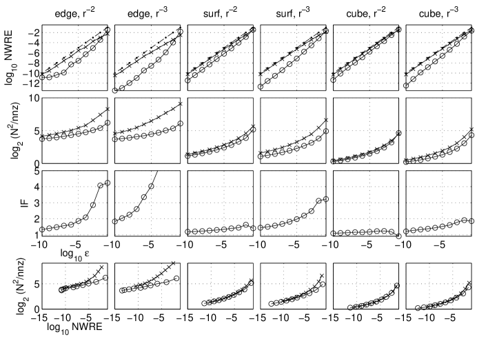
Figure 4 shows the behavior of the two methods for $p=2,3$ and the three geometries when the requested tolerance is varied. The first three rows are as in the earlier figures except that the abscissa is the tolerance rather than problem size. For easy reference, in the first row requested tolerance is also indicated by the line having dots. The fourth row plots compression against achieved error. On these test problems, MREM achieves greater compression than BREM even when the achieved errors are the same.

4.2 A problem in geophysics

The problem that motivated this work is one in geophysics. We are modeling the evolution of slip on a fault in an elastic half space. One part of the computation is a matrix-vector product relating slip on the fault to stress. The fault is discretized by rectangular patches, and stress at the center of all patches due to unit slip on one patch is computed using the rectangular dislocation code of okada92 . The matrix is approximated by an H-matrix. We performed a test on a fault discretized by $156\times 402$ rectangles with a tolerance of $10^{-5}$. For respectively BREM and MREM, the actual errors are $1.28\times 10^{-8}$ and $1.71\times 10^{-6}$; the compression factors are $16.89$ and $75.74$, for an improvement factor of $4.48$.

Fig. 1: Particles are distributed uniformly on the edges of a cube.

Fig. 2: Particles are distributed uniformly on the surface of a cube.

Fig. 3: Particles are distributed uniformly inside a cube.

Fig. 4: The requested tolerance $\varepsilon$ is varied. The number of particles is approximately $N=2^{13}$.

5 Conclusions

For many problems, MREM produces a more efficient approximation than BREM for a requested error tolerance by producing an approximation $\bar{B}$ that is little more accurate than is requested. MREM rarely produces a less efficient approximation, and then only by a small amount. Improvement factors are often between $1.5$ and $5$. The improvement factor increases with the dominance of the diagonal. For problems in which the order of the singularity is $1$, MREM’s results are almost exactly the same as BREM’s. For higher-order problems, MREM is consistently better by a substantial and practically useful amount. MREM is also better than BREM for high-order singularities even when achieved, rather than requested, error is considered.

Using MREM rather than BREM requires the extra work to estimate $\|B\|_{\text{F}}$ if it is not known. In our experiments, $\|B\|_{\text{F}}$ is estimated in a time that is approximately $1\%$ of the total construction time. Because the work to find a block LRA increases with the block tolerance, MREM is faster than BREM on any problem in which the resulting compression is greater by at least a small amount.

The similarity in block tolerances suggests that the compression factors resulting from MREM and MREMmax can be expected to scale with problem size and tolerance similarly. However, SVD recompression is far more efficient when using MREM. We conclude that one should consider using MREM when a problem’s singularity has order greater than $1$.

Acknowledgements. I would like to thank Prof. Eric Darve, Dept. of Mech. Eng., Stanford University, for reading a draft of this paper and a helpful discussion; and Prof. Paul Segall, Dept. of Geophysics, Stanford University, for supporting this research.

References

- (1) M. Bebendorf, Hierarchical Matrices: A Means to Efficiently Solve Elliptic Boundary Value Problems, Springer, 2008.
- (2) M. Bebendorf and S. Rjasanow, Adaptive low-rank approximation of collocation matrices, Computing, 70 (2003), pp. 1–24.
- (3) S. Börm, Adaptive variable-rank approximation of general dense matrices, SIAM J. Sci. Comput., 30 (2007), pp. 148–168.
- (4) S. Börm and L. Grasedyck, Hybrid cross approximation of integral operators, Numerische Mathematik, (2005).
- (5) S. Börm, L. Grasedyck, and W. Hackbusch, Hierarchical matrices. Lecture Notes, 2003.
- (6) Y. Okada, Internal deformation due to shear and tensile faults in a half-space, Bull. Seism. Soc. Am., 82 (1992).
- (7) S. Rjasanow and O. Steinbach, The Fast Solution of Boundary Integral Equations (Mathematical and Analytical Techniques with Applications to Engineering), Springer, 2007.
- (8) S. A. Sauter, Variable order panel clustering, Computing, 64 (2000), pp. 223–261.