Matrix-Free Approximate Equilibration

Abstract

The condition number of a diagonally scaled matrix, for appropriately chosen scaling matrices, is often less than that of the original. Equilibration scales a matrix so that the scaled matrix’s row and column norms are equal. Scaling can be approximate. We develop approximate equilibration algorithms for nonsymmetric and symmetric matrices having signed elements that access a matrix only by matrix-vector products.

1 Introduction

For a square, nonnegative, real, nonsymmetric matrix $B$, equilibration in the 1-norm finds $x,y>0$ such that $XBy=e$ and $YB^{T}x=e$, where $X=\text{diag}(x)$ and similarly for other vectors, and $e$ is the vector of all ones. Hence $XBY$ is doubly stochastic. For a symmetric matrix, symmetric equilibration finds $x>0$ such that $XBx=e$. If $B=A\circ A$ for $A$ a real, possibly signed, matrix, where $\circ$ denotes the element-wise product, then these equations equilibrate $A$ in the 2-norm. Equilibration in the 2-norm is often called binormalization. Approximate equilibration scales a matrix so that its row and column norms are almost equal. Both the exactly and approximately equilibrated matrices often have smaller condition numbers than the original. In this paper we always use the 2-norm condition number. Equilibration is particularly usefully applied to matrices for which simpler diagonal scaling methods fail: for example, to indefinite symmetric matrices. In Section 2, we compare equilibration with Jacobi scaling when applied to symmetric matrices.

In some problems, accessing elements of a matrix is expensive. What are often called matrix-free algorithms access a matrix only by matrix-vector products. If $A$ is a matrix having nonnegative elements, then many algorithms already exist to equilibrate $A$ using only matrix-vector products: for example, the Sinkhorn-Knopp iteration. But if $A$ has signed elements, then one must obtain $|A|$ to use these algorithms, which requires accessing the elements of $A$. In Section 3, we develop matrix-free approximate equilibration algorithms for square nonsymmetric and symmetric matrices having signed elements, and we report the results of numerical experiments with these algorithms in Section 4.

2 Diagonal scaling of symmetric matrices

Fig. 1: Numerical study of conditioning of symmetric matrices. The four plots show condition number of the Jacobi-scaled (top) and binormalized (bottom) symmetric positive definite (left) and indefinite (right) matrix as a function of the condition number of the unscaled matrix.

Jacobi scaling pre- and post-multiplies a square, usually symmetric positive definite (spd) matrix by a diagonal matrix such that the scaled matrix has unit diagonal elements.

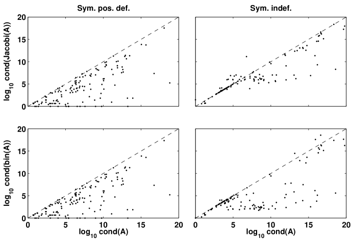
Numerical experiments show that the condition number of the equilibrated or Jacobi-scaled matrix is often considerably less than that of the original matrix. Figure 1 shows the results of a numerical experiment using 323 symmetric matrices from the University of Florida Sparse Matrix Collection [7]; see Section 4 for further details on the data set. The matrices used in this experiment have sizes 10 to 36441, with a median size of 5000. Figure 1 shows the condition number of the scaled matrix as a function of that of the unscaled matrix. Two diagonal scaling methods are used: Jacobi (top) and binormalization (bottom). Matrices are divided into positive definite (left) and indefinite (right).

This experiment shows that if a matrix is spd, then equilibration and Jacobi scaling reduce the condition number by about the same amount; indeed, the two corresponding plots are almost identical. It also shows that when the two methods are applied to an indefinite matrix—in the case of Jacobi scaling, replacing a zero diagonal element with a one—the condition number of the Jacobi-scaled matrix is likely to be substantially greater than that of the equilibrated matrix. For these reasons, equilibration of symmetric indefinite matrices can be thought of as a generalization of Jacobi scaling of spd matrices, raising the question of the relationship between the two scaling methods when applied to spd matrices.

Let $A$ be an $n\times n$ spd matrix whose diagonal elements are all one. Let $\kappa(\cdot)$ denote the 2-norm condition number of a matrix. Van der Sluis showed that $\kappa(A)\leq n\min_{d}\kappa(DAD)$ (Theorem 4.1 of [21]) and that if $A$ has at most $q$ nonzero elements in any row, then $\kappa(A)\leq q\min_{d}\kappa(DAD)$ (Theorem 4.3 of [21]). A matrix $C$ has Young’s property A if there exists a permutation matrix $P$ such that

$$PCP^{T}=\begin{pmatrix}D_{1}&C_{1}\\ C_{2}&D_{2}\end{pmatrix}$$

and $D_{1}$ and $D_{2}$ are square diagonal matrices. Forsthye and Straus showed that if the matrix $A$ has in addition Young’s property A, then $\kappa(A)=\min_{d}\kappa(DAD)$ (Theorem 4 of [9]). In summary, these three theorems state that Jacobi scaling is within a factor of $n$, $q$, or 1 of optimal among all diagonal scaling matrices.

If $A$ is spd, then so is $B\equiv A\circ A$ by the Schur Product Theorem (see, for example, Theorem 7.5.3 of [10]). Suppose $A$ has unit diagonal elements. Then so does $B$. Moreover, $B_{ij}<1$ for $i\neq j$. Suppose Jacobi scaling—replacing a zero diagonal element with a one—has been applied to an $n\times n$ symmetric matrix $\bar{A}$ to yield the matrix $A$, and again let $B\equiv A\circ A$. Consider the vector of row sums $s\equiv Be$. If $\bar{A}$ is indefinite, $0\leq s_{i}<\infty$. If $\bar{A}$ is spd, as every diagonal element of $B$ is 1, $s_{i}\geq 1$; and as every off-diagonal element $B_{ij}<1$, $s_{i}<n$.

Let $\mu(v)$ be the mean of the elements of an $n$-vector $v$ and $\text{var}(v)$ the variance: $\text{var}(v)\equiv n^{-1}\sum_{i}(v_{i}-\mu(v))^{2}$. If a matrix is binormalized, then the variance of the vector of its row 2-norms is 0. If $\bar{A}$ is indefinite, $\text{var}(s)$ can be arbitrarily large. But if $A$ is spd, then $\text{var}(s)<(n-1)^{2}$. For as each $1\leq s_{i}<n$, $(s_{i}-\mu(s))^{2}<(n-1)^{2}$, and so $n^{-1}\sum_{i}(s_{i}-\mu(s))^{2}<n^{-1}\sum_{i}(n-1)^{2}=(n-1)^{2}$.

From the other direction, an immediate corollary of inequality 2 in [15] is that if an spd matrix $\bar{A}$ is equilibrated in the 2-norm to form $\tilde{A}$, then $n^{-1/2}<\tilde{A}_{ii}\leq 1$ (the upper bound follows immediately from equilibration to unit row and column 1-norms); if $\bar{A}$ is indefinite, then of course $-1\leq\tilde{A}_{ii}\leq 1$.

In summary, if a matrix is spd, Jacobi scaling produces a matrix that is not arbitrarily far from being binormalized, and binormalization produces a matrix whose diagonal elements are bounded below and above by positive numbers. The bounds depend on the size of the matrix. If a matrix is symmetric indefinite, then neither statement holds.

3 Algorithms

Sinkhorn and Knopp analyzed the convergence properties of the iteration (1):

$$r^{k+1}=(Bc^{k})^{-1},\quad c^{k+1}=(B^{T}r^{k+1})^{-1}.$$ (1)

The reciprocal is applied by element. $c^{0}$ is a vector whose elements are all positive. According to Knight [12], the iteration was used as early as the 1930s.

Parlett and Landis [17] generalized Sinkhorn and Knopp’s convergence analysis and developed several new algorithms, one of which, EQ, substantially outperformed the Sinkhorn-Knopp iteration on a test set. Khachiyan and Kalantari [11] used Newton’s method to scale positive semidefinite symmetric matrices. Livne and Golub [16] developed algorithms for symmetric and nonsymmetric matrices based on the Gauss-Seidel-Newton method. Knight and Ruiz [13] devised an algorithm based on an inexact Newton method that uses the conjugate gradients iteration.

Nonuniqueness of equilibration in the infinity norm motivates multiple algorithms that consider both efficiency and quality of the scaling under criteria other than the infinity norms of the rows and columns. A matrix can be scaled in the infinity norm if it has no zero rows or columns. The simplest nonsymmetric algorithm is first to scale the rows (columns), then to scale the columns (rows). After the first scaling, the largest number in the matrix is 1, and the second scaling cannot produce numbers that are larger than 1. Therefore, scaling is achieved after one iteration. Bunch [4] developed an algorithm that equilibrates any symmetric matrix in the infinity norm. More recently, Ruiz [19] developed another iteration that compares favorably with Bunch’s algorithm. He extended the method to 1- and 2-norms and showed convergence results for these algorithms as strong as, and based on, those by Parlett and Landis [17] for their algorithms.

Each of these algorithms is iterative and yields a sequence of matrices converging to a doubly stochastic matrix. A user can terminate the iteration early to yield an approximately equilibrated matrix; hence these algorithms may be viewed as approximate equilibration algorithms.

To date, it appears that all scaling algorithms for matrices having signed elements require access to the elements of the matrix. If $A$ is nonnegative, the situation is much different; for example, the Sinkhorn-Knopp algorithm requires only the matrix-vector products (mvp) $Ax$ and $A^{T}x$. For general matrices, algorithms need at least mvp of the form $|A|x$ (1-norm), $(A\circ A)x$ (2-norm), or similar expressions, and their transposes. We introduce approximate scaling algorithms for equilibration in the 2-norm that require only the mvp $Ax$ and $A^{T}x$, where $x$ is a random vector. Algorithms that compute the mvp with a random vector have been developed to solve other problems. For example, Bekas, Kokiopoulou, and Saad [1] developed a method to estimate the diagonal elements of a matrix; and Chen and Demmel [5], to balance a matrix prior to computing its eigenvalues. Our algorithms also have a connection to the methods of stochastic approximation [14].

We want to emphasize that because the algorithms we propose access a matrix having signed elements only through a sequence of mvp, we cannot expect them to be faster than, or even as fast as, algorithms that access the elements directly when applied to matrices for which direct access to the elements is possible and efficient. Our algorithms are useful only if a matrix has signed elements that are impossible or inefficient to access directly; it appears there are not algorithms already available to solve this problem. It is also desirable that only a small number, relative to the size of the matrix, of mvp are required.

3.1 Existence and uniqueness

A matrix has support if a positive main diagonal exists under a column permutation; a matrix having this property is equivalently said to be structurally nonsingular [8]. A square matrix has total support if every nonzero element occurs in the positive main diagonal under a column permutation. A matrix has total support if and only if there exists a doubly stochastic matrix having the same zero pattern [18]. A matrix $A$ is partly decomposable if there exist permutation matrices $P$ and $Q$ such that

$$PAQ=\begin{pmatrix}E&0\\ C&D\end{pmatrix},$$ (2)

where $E$ and $D$ are square matrices. A square matrix is fully indecomposable if it is not partly decomposable. A fully indecomposable matrix has total support [2]. A matrix $A$ is reducible if there exists a permutation matrix $P$ such that $PAP^{T}$ has the matrix structure in (2); otherwise, $A$ is irreducible. For convenience, a matrix is said to be scalable if it can be equilibrated.

Theorem 1 (Sinkhorn and Knopp [20]).

Let $B$ be a nonnegative square matrix.

1. There exist positive diagonal matrices $R$ and $C$ such that $F\equiv RBC$ is doubly stochastic—briefly, $B$ is scalable—if and only if $B$ has total support.

2. If $B$ is scalable, then $F$ is unique.

3. $R$ and $C$ are unique up to a scalar multiple if and only if $B$ is fully indecomposable.

4. The Sinkhorn-Knopp iteration yields a sequence of matrices that converges to a unique doubly stochastic matrix, for all initial $r,c>0$, if and only if $B$ has support. If $B$ has support that is not total, then $R$ and $C$ have elements that diverge.

Parts 1–3 were independently discovered in [3].

Theorem 2 (Csima and Datta [6]).

A symmetric matrix is symmetrically scalable if and only if it has total support.

The necessary and sufficient condition of total support in Theorem 2 is identical to that in part 1 of Theorem 1. The necessary part follows directly from part 1, but proving the sufficiency part requires several steps not needed in the nonsymmetric case.

Section 3 of [12] discusses the symmetric iteration

$$x^{k+1}=(Bx^{k})^{-1}$$ (3)

for symmetric $B$ and sketches a proof of convergence. Not directly addressed is that the iterates $x^{k}$ can oscillate and reducible $B$.

If $B$ is irreducible, this oscillation is straightforward and benign. The resulting scaled matrix is a scalar multiple of a doubly stochastic one. For example, suppose $\bar{B}=1$ and $x^{0}=2$. Then for $k$ even, $x^{k}=2$, and for $k$ odd, $x^{k}=1/2$. In general, if symmetric $B$ is irreducible, $X^{k}BX^{k+1}$ converges to a doubly stochastic matrix, while $X^{2k}BX^{2k}$ and $X^{2k+1}BX^{2k+1}$ converge to scalar multiples of a doubly stochastic matrix, and these scalars are reciprocals of each other.

Somewhat more complicated is reducible $B$. For example, consider the matrix $\bar{B}=\text{diag}(1\ 2)^{T}$. If $x^{0}=e$, the even iterates remain $e$ while the odd iterates are $v\equiv(1\ 1/2)^{T}$. $I\bar{B}V$ is doubly stochastic, but $v$ is not proportional to $e$. Moreover, $V\bar{B}V$ is not simply a scalar multiple of a doubly stochastic matrix. This nonconvergence is also benign. A reducible symmetric matrix $B$ can be symmetrically permuted to be block diagonal with each block irreducible. Hence the equilibration problem is decoupled into as many smaller problems. We can construct a symmetric equilibrating vector $x$ from the nonsymmetric equilibrating vectors $r$ and $c$ by setting $x=\sqrt{rc}$. For suppose $r$ and $c$ equilibrate $B$ by $RBC$. Let ${\cal I}$ be the indices corresponding to an irreducible block. Then $r({\cal I})\propto c({\cal I})$ and the block $X({\cal I},{\cal I})B({\cal I},{\cal I})X({\cal I},{\cal I})$ is doubly stochastic. For $\bar{B}$, the symmetric equilibration vector is $\sqrt{ev}=(1\ 1/\sqrt{2})^{T}$.

These observations suggest that we should write the symmetric Sinkhorn-Knopp iteration as

$$y^{k+1}=(By^{k})^{-1},\quad x^{k+1}=\sqrt{y^{k+1}y^{k}}.$$ (4)

Since $x^{k}$ does not actually play a role in the iteration, in practice, the square root operation needs to be applied only after the final iteration to yield the scaling matrix.

3.2 Stochastic equilibration

Our algorithms are based on the Sinkhorn-Knopp iteration. The Sinkhorn-Knopp iteration performs the mvp $Bx$ and $B^{T}x$ for a nonnegative matrix $B$. If $A$ is a matrix having signed elements, then $B_{ij}=|A_{ij}|^{p}$ for $p\geq 1$ for equilibration in the $p$-norm, and so $B$ is not available if one does not have access to the elements of $A$. The key idea, similar to that in [5], in our algorithms is to compute $Bx$ approximately by using an mvp with $A$ rather than $B$, where $B\equiv A\circ A$, and similarly for $B^{T}x$.

Let $a\in\mathbb{R}^{n}$. If the elements of the random vector $u\in\mathbb{R}^{n}$ have zero mean, positive and finite variance, and are iid, then $\text{E}\,(a^{T}u)^{2}=\eta\text{E}\,a^{T}a$ for finite $\eta>0$, where E denotes expectation. For as $\text{E}\,u_{i}u_{j}=0$ if $i\neq j$, $\text{E}\,(\sum_{j}a_{j}u_{j})^{2}=\text{E}\,\sum_{j}a_{j}^{2}u_{j}^{2}=\eta\sum_{j}a_{j}^{2}$, where $\eta=\text{E}\,u_{j}^{2}>0$ is finite. See [5] for more on this and related expectations. We use this fact to approximate $Bx$ by computing the mvp $AX^{1/2}u$:

$$\text{E}\,(AX^{1/2}u)^{2}=\eta((AX^{1/2})\circ(AX^{1/2}))e=\eta(A\circ A)Xe=\eta Bx.$$ (5)

To increase the accuracy of the approximation to $Bx$, one could compute the mean of multiple mvp $AX^{1/2}u$. Then one could construct an approximate scaling algorithm by replacing the exact computation $Bx$ with this estimate, and similarly for $B^{T}x$, in the Sinkhorn-Knopp algorithm. However, the method of stochastic approximation [14] suggests a better approach. In stochastic approximation, the exact iteration $x^{k+1}=x^{k}+\omega^{k}f(x^{k})$ is replaced by the stochastic iteration $x^{k+1}=x^{k}+\omega^{k}\tilde{f}(x^{k})$, where $\text{E}\,\tilde{f}(x^{k})=f(x^{k})$ and $x$ is sought such that $f(x)=0$. Rather than explicitly average multiple realizations of $\hat{f}(x^{k})$ at each iteration, the stochastic approximation iteration controls the relative weight of $\hat{f}$ through $\omega^{k}$ and alters the iterate $x^{k}$ at each evaluation of $\hat{f}$.

Let $\rho\equiv r^{-1}$, $\gamma\equiv c^{-1}$, and $0<\omega^{k}<1$. Consider the iteration

$$\rho^{k+1} =(1-\omega^{k})\frac{\rho^{k}}{\|\rho^{k}\|_{1}}+\omega^{k}\frac{Bc^{k}}{\|Bc^{k}\|_{1}}$$ (6)

$$\gamma^{k+1} =(1-\omega^{k})\frac{\gamma^{k}}{\|\gamma^{k}\|_{1}}+\omega^{k}\frac{B^{T}r^{k+1}}{\|B^{T}r^{k+1}\|_{1}}.$$

This iteration takes a convex combination of the reciprocal of an iterate and the Sinkhorn-Knopp update when each is normalized by its 1-norm. Let $u^{k}$ and $v^{k}$ be random vectors as before. For the vector $x$, $(x)^{2}$ is the element-wise square. Substituting (5) into this iteration, we obtain the stochastic iteration

$$y^{k} =(A(C^{k})^{1/2}u^{k})^{2}$$

$$\rho^{k+1} =(1-\omega^{k})\frac{\rho^{k}}{\|\rho^{k}\|_{1}}+\omega^{k}\frac{y^{k}}{\|y^{k}\|_{1}}$$ (7)

$$z^{k} =(A^{T}(R^{k+1})^{1/2}v^{k})^{2}$$

$$\gamma^{k+1} =(1-\omega^{k})\frac{\gamma^{k}}{\|\gamma^{k}\|_{1}}+\omega^{k}\frac{z^{k}}{\|z^{k}\|_{1}}.$$

We implement this iteration in the Matlab function snbin.

⬇

function [r c] = snbin(A,nmv,m,n)

% Stochastic matrix-free binormalization for nonsymmetric real A.

% A is a matrix or function handle. If it is a function handle,

% then v = A(x) returns A*x and v = A(x,‘trans’) returns A’*x.

% nmv is the number of forward and transpose matrix-vector

% product pairs to perform.

% m,n is the size of the matrix. It is necessary to specify

% these only if A is a function handle.

% diag(r) A diag(c) is approximately binormalized (to a scalar).

op = isa(A,‘function_handle’);

␣␣␣␣␣␣␣if(~op)␣[m␣n]␣=␣size(A);␣end

␣␣␣␣␣␣␣r␣=␣ones(m,1);␣c␣=␣ones(n,1);

␣␣␣␣␣␣␣for(k␣=␣1:nmv)

␣␣␣␣␣␣␣␣␣%␣omega^k

␣␣␣␣␣␣␣␣␣alpha␣=␣(k␣-␣1)/nmv;

␣␣␣␣␣␣␣␣␣omega␣=␣(1␣-␣alpha)*1/2␣+␣alpha*1/nmv;

␣␣␣␣␣␣␣␣␣%␣rows

␣␣␣␣␣␣␣␣␣s␣=␣randn(n,1)./sqrt(c);

␣␣␣␣␣␣␣␣␣if(op)␣y␣=␣A(s);␣else␣y␣=␣A*s;␣end

␣␣␣␣␣␣␣␣␣r␣=␣(1-omega)*r/sum(r)␣+␣omega*y.^2/sum(y.^2);

␣␣␣␣␣␣␣␣␣%␣columns

␣␣␣␣␣␣␣␣␣s␣=␣randn(m,1)./sqrt(r);

␣␣␣␣␣␣␣␣␣if(op)␣y␣=␣A(s,‘trans’);␣else␣y␣=␣(s’*A)’;␣end

␣␣␣␣␣␣␣␣␣c␣=␣(1-omega)*c/sum(c)␣+␣omega*y.^2/sum(y.^2);

␣␣␣␣␣␣␣end

␣␣␣␣␣␣␣r␣=␣1./sqrt(r);␣c␣=␣1./sqrt(c);

Our choice of the sequence $\omega^{k}$ is based on numerical experiments; the sequence encourages large changes in $d/\|d\|_{1}$ when $k$ is small and smaller changes when $k$ is large.

Iteration (6) forms a linear combination of $\rho^{k}$ and $Bc^{k}$. One might consider instead forming a linear combination of $r^{k}$ and $(Bc^{k})^{-1}$. In the iteration we use, a reciprocal is taken after forming a linear combination of the iterate and a random quantity; in contrast, in this alternative, it is taken before, and of the random quantity. Consequently, the stochastic iteration corresponding to this alternative iteration is less stable than (7).

A straightforward algorithm for the symmetric problem applies snbin to the symmetric matrix $B$ and then returns $\sqrt{rc}$. But numerical experiments suggest we can do better. For irreducible matrices, the denominators $\|d^{k}\|_{1}$ and $\|Bx^{k}\|_{1}$ in the iteration

$$d^{k+1}=(1-\omega^{k})\frac{d^{k}}{\|d^{k}\|_{1}}+\omega^{k}\frac{Bx^{k}}{\|Bx^{k}\|_{1}}$$

remove the benign oscillation we observed in Section 3.1; therefore, adjacent iterates, rather than every other one as in (6), can be combined in a convex sum. This second approach speeds convergence. But it is not sufficient when applied to reducible matrices. Numerical experiments support using the second approach for early iterations, when making progress quickly is important, and then switching to the first approach to refine the scaling matrix. We implement this strategy in ssbin.

⬇

function x = ssbin(A,nmv,n)

% Stochastic matrix-free binormalization for symmetric real A.

% A is a symmetric real matrix or function handle. If it is a

% function handle, then v = A(x) returns A*x.

% nmv is the number of matrix-vector products to perform.

% [n] is the size of the matrix. It is necessary to specify n

% only if A is a function handle.

% diag(x) A diag(x) is approximately binormalized (to a scalar).

op = isa(A,’function_handle’);

␣␣␣␣␣␣␣if(~op)␣n␣=␣size(A,1);␣end

␣␣␣␣␣␣␣d␣=␣ones(n,1);␣dp␣=␣d;

␣␣␣␣␣␣␣for(k␣=␣1:nmv)

␣␣␣␣␣␣␣␣␣%␣Approximate␣matrix-vector␣product

␣␣␣␣␣␣␣␣␣u␣=␣randn(n,1);

␣␣␣␣␣␣␣␣␣s␣=␣u./sqrt(dp);

␣␣␣␣␣␣␣␣␣if(op)␣y␣=␣A(s);␣else␣y␣=␣A*s;␣end

␣␣␣␣␣␣␣␣␣%␣omega^k

␣␣␣␣␣␣␣␣␣alpha␣=␣(k␣-␣1)/nmv;

␣␣␣␣␣␣␣␣␣omega␣=␣(1␣-␣alpha)*1/2␣+␣alpha*1/nmv;

␣␣␣␣␣␣␣␣␣%␣Iteration

␣␣␣␣␣␣␣␣␣d␣=␣(1-omega)*d/sum(d)␣+␣omega*y.^2/sum(y.^2);

␣␣␣␣␣␣␣␣␣if␣(k␣<␣min(32,floor(nmv/2)))␣%␣Ignore␣reducibility.

␣␣␣␣␣␣␣␣␣␣␣dp␣=␣d;

␣␣␣␣␣␣␣␣␣else␣␣␣␣␣%␣This␣block␣makes␣ssbin␣behave␣like␣snbin.

␣␣␣␣␣␣␣␣␣␣␣tmp␣=␣dp;␣dp␣=␣d;␣d␣=␣tmp;␣␣␣␣␣␣␣␣%␣Swap␣dp␣and␣d.

␣␣␣␣␣␣␣␣␣end

␣␣␣␣␣␣␣end

␣␣␣␣␣␣␣x␣=␣1./(d.*dp).^(1/4);␣␣␣␣␣␣␣␣%␣In␣case␣B␣is␣reducible

The final line implements the square root in (4).

In most iterative algorithms, a measure of the merit of an iterate that requires little work to evaluate relative to the work in an iteration influences the behavior of the algorithm. In our algorithms, any procedure to assess the merit of an iterate would require additional mvp, likely wasting work. Hence the parameter values in the loop of each algorithm are fixed independent of problem.

4 Numerical experiments

Fig. 2: Convergence histories for two symmetric problems having sizes 3564 (left) and 226340 (right). Ten solid lines show individual realizations of the algorithm. The dashed line corresponds to snbin. The dotted line corresponds to not switching to snbin-like behavior.

Fig. 3: Ratio for the original and scaled nonsymmetric matrix vs. matrix size $N$, after the indicated number of iterations, for 741 matrices.

Fig. 4: Condition number of the scaled nonsymmetric matrix vs. condition number of the original matrix for 519 matrices (matrices having $N\leq 2\times 10^{4}$).

Fig. 5: Ratios for 466 symmetric matrices. Results for only $K=128$ are shown; trends in $K$ follow those for the nonsymmetric problems.

Fig. 6: Condition numbers for 221 symmetric matrices (matrices having $N\leq 2\times 10^{4}$).

Fig. 7: A closer look at the ratio as a function of $N$ for $K=128$ iterations for nonsymmetric (left) and symmetric (right) matrices.

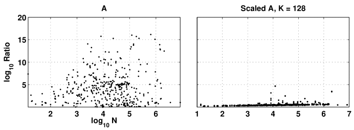
In our numerical experiments, two quantities of the scaled matrices are measured: condition number if the matrix is not too large; and the ratio of the largest to smallest row 2-norms (in the nonsymmetric case, row or column, depending on which gives a larger number), hereafter designated as the ratio.

We test snbin and ssbin in Matlab on matrices in the University of Florida Sparse Matrix Collection [7]; these are obtained by the following queries:

⬇

index = UFget(‘refresh’);

␣␣␣␣␣%␣Symmetric

␣␣␣␣␣sids␣=␣find(~index.isBinary␣&␣index.numerical_symmetry␣==␣1␣&…

␣␣␣␣␣␣␣␣␣␣␣␣␣␣␣␣␣index.sprank␣==␣index.nrows␣&␣index.isReal);

␣␣␣␣␣%␣Square␣nonsymmetric

␣␣␣␣␣nids␣=␣find(~index.isBinary␣&␣index.numerical_symmetry␣<␣1␣&…

␣␣␣␣␣␣␣␣␣␣␣␣␣␣␣␣␣index.nrows␣==␣index.ncols␣&…

␣␣␣␣␣␣␣␣␣␣␣␣␣␣␣␣␣index.sprank␣==␣index.nrows␣&␣index.isReal);

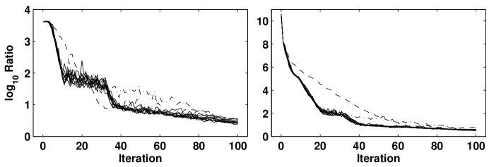
First we investigate the behavior of ssbin on two problems. Figure 2 shows the convergence history, starting with the unaltered matrix, for 12 runs of ssbin on two symmetric problems. The smaller has size 3564; the larger has size 226340. $\log_{10}$ ratio is used to measure convergence. The ten closely clustered solid curves correspond to the nominal algorithm. The dashed curve indicates the slower convergence of simply applying snbin. The dotted curve shows the problem with not eventually switching to snbin-like behavior to address reducibility. The plateau in the solid curves ends at iteration 32, when the switch is made. The ten solid curves are closely clustered, indicating the variance in the algorithm’s output is small for any number of requested mvp.

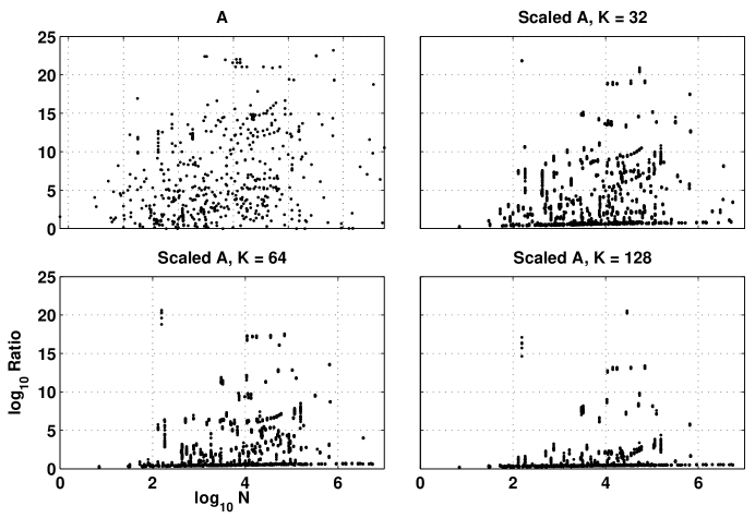
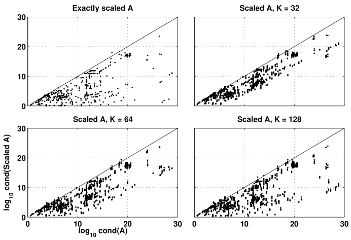
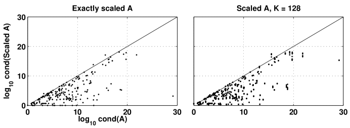
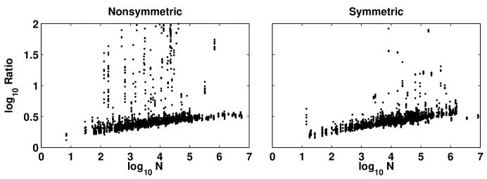
In the performance experiments, for each matrix, the algorithm is run five times for $K=32$, $64$, and $128$ iterations. Results are shown in Figures 3 and 4 for nonsymmetric matrices and 5 and 6 for symmetric matrices. Figure 3 shows that the ratio tends to decrease with $K$, as one expects. The ratio for the scaled problem, given fixed $K$, grows slowly with problem size $N$. Figure 7 investigates this aspect more closely. It shows details for the case of $K=128$ iterations for nonsymmetric (left) and symmetric (right) matrices. Over a range of matrix sizes of more than six orders of magnitude, the final ratio often ranges from between $1.5$ and $6$. Figures 4 and 6 show that the condition number of the scaled matrix is almost always, and often substantially, smaller than that of the original matrix: any point that falls below the diagonal line corresponds to a reduction in condition number. The top-left plots of Figures 4 and 6 show the condition numbers of the exactly scaled matrices; the ratios are 1, of course. In the plots corresponding to the stochastic algorithms, what appears to be a point is in fact a cluster of the five points resulting from the five separate runs. The tightness of these clusters again implies that the variance of the outputs of these algorithms is quite small.

These experiments suggest that ssbin and snbin are effective matrix-free approximate equilibration algorithms: a small number—relative to the size of the matrix—of matrix-vector products is sufficient to approximately equilibrate the matrix. One application is to scale a matrix whose elements require too much work to access directly prior to using a Krylov-subspace iteration to solve a linear system. We recommend performing approximately 100 iterations, which corresponds to 100 matrix-vector products in the symmetric case and 200 in the nonsymmetric.

References

- [1] C. Bekas, E. Kokiopoulou, and Y. Saad, An estimator for the diagonal of a matrix, Appl. Num. Math., 57 (2007), pp. 1214–1229.
- [2] R. A. Brualdi, Matrices of 0’s and 1’s with total support, J. of Comb. Theory, 28 (1980), pp. 249–256.
- [3] R. A. Brualdi, S. V. Parter, and H. Schneider, The diagonal equivalence of a nonnegative matrix to a stochastic matrix, J. Math. Anal. Appl., 16 (1966), pp. 31–50.
- [4] J. R. Bunch, Equilibration of symmetric matrices in the max-norm, JACM, 18 (1971), pp. 566–572.
- [5] T.-Y. Chen and J. W. Demmel, Balancing sparse matrices for computing eigenvalues, Lin. Alg. Appl., 309 (2000), pp. 261–287.
- [6] J. Csima and B. N. Datta, The DAD theorem for symmetric non-negative matrices, J. Comb. Theory, 12 (1972), pp. 147–152.
-
[7]
T. A. Davis, The University of Florida sparse matrix
collection.
http://www.cise.ufl.edu/research/sparse/matrices. - [8] , Direct Methods for Sparse Linear Systems, SIAM, 2006.
- [9] G. E. Forsythe and E. G. Straus, On best conditioned matrices, Proc. Amer. Math. Soc., 6 (1955), pp. 340–345.
- [10] R. A. Horn and C. R. Johnson, Matrix Analysis, Cambridge, U.K.: Cambridge Univ. Press, 1985.
- [11] L. Khachiyan and B. Kalantari, Diagonal matrix scaling and linear programming, SIAM J. on Optim., 2 (1992), pp. 668–672.
- [12] P. A. Knight, The Sinkhorn-Knopp algorithm: Convergence and applications, SIMAX, 30 (2008), pp. 261–275.
- [13] P. A. Knight and D. Ruiz, A fast algorithm for matrix balancing, in Web Information Retrieval and Linear Algebra Algorithms, 2007.
- [14] H. J. Kushner and G. Yin, Stochastic approximation and recursive algorithms and applications, (2003).
- [15] O. E. Livne, Diagonal dominance of SPD matrices, tech. report, Stanford University, 2004.
- [16] O. E. Livne and G. H. Golub, Scaling by binormalization, Numer. Alg., 35 (2004), pp. 97–120.
- [17] B. N. Parlett and T. L. Landis, Methods for scaling to double stochastic form, Lin. Alg. Appl., 48 (1982), pp. 53–79.
- [18] L. Perfect and L. Mirsky, The distribution of positive elements in doubly stochastic matrices, J. London Math. Soc., 40 (1965), pp. 689–698.
- [19] D. Ruiz, A scaling algorithm to equilibrate both rows and column norms in matrices, Tech. Report RT/APO/01/4, ENSEEIHT-IRIT, 2001.
- [20] R. Sinkhorn and P. Knopp, Concerning nonnegative matrices and doubly stochastic matrices, Pacific J. Math., 21 (1967), pp. 343–348.
- [21] A. van der Sluis, Condition numbers and equilibration of matrices, Numer. Math., 14 (1969), pp. 14–23.