CERN-PH-TH/2011-225
Edinburgh 2011/29
FR-PHENO-2011-018
IFUM-985-FT
TTK-11-50
Precision NNLO determination of
using an unbiased global parton set
The NNPDF Collaboration: Richard D. Ball1, Valerio Bertone2, Luigi Del Debbio1,
Stefano Forte3,4, Alberto Guffanti5, José I. Latorre6, Simone Lionetti3, Juan Rojo7 and Maria Ubiali8.
1 Tait Institute, University of Edinburgh,
JCMB, KB, Mayfield Rd, Edinburgh EH9 3JZ, Scotland
2 Physikalisches Institut, Albert-Ludwigs-Universität Freiburg,
Hermann-Herder-Straße 3, D-79104 Freiburg i. B., Germany
3 Dipartimento di Fisica, Università di Milano and
4 INFN, Sezione di Milano,
Via Celoria 16, I-20133 Milano,
Italy
5 The Niels Bohr International Academy and Discovery Center,
The Niels Bohr Institute, Blegdamsvej 17, DK-2100 Copenhagen, Denmark
6 Departament d’Estructura i Constituents de la Matèria,
Universitat de Barcelona,
Diagonal 647, E-08028 Barcelona, Spain
7 PH Department, TH Unit, CERN, CH-1211 Geneva 23, Switzerland
8 Institut für Theoretische Teilchenphysik und Kosmologie, RWTH Aachen University,
D-52056 Aachen, Germany
Abstract:
We determine the strong coupling at NNLO in perturbative QCD using the global dataset input to the NNPDF2.1 NNLO parton fit: data from neutral and charged current deep-inelastic scattering, Drell-Yan, vector boson production and inclusive jets. We find , where the statistical uncertainty comes from the underlying data and uncertainties due to the analysis procedure are negligible. We show that the distribution of values preferred by different experiments in the global fit is statistically consistent, without need for rescaling uncertainties by a “tolerance” factor. We show that if deep-inelastic data only are used, the best-fit value of is somewhat lower, but consistent within one sigma with the global determination. We find that the shift between the NLO and NNLO values of is , and we estimate the uncertainty from higher-order corrections to be .
We have recently shown [1] that a surprisingly precise determination of using next-to-leading order perturbative QCD can be obtained from the dependence on the value of the strong coupling of the quality of a global unbiased fit [2] of parton distributions to deep-inelastic, Drell-Yan and inclusive jet data. This result was somewhat unexpected. Indeed, previous determinations of from global parton fits based on the idea of treating as a fit parameter [3, 4, 5] obtained larger uncertainties, and the precision of Ref. [1] is achieved even though the underlying PDF parametrization [2] adopted there is so general that the concept of a global best fit is no longer useful, and one must instead consider the fit quality (as measured by the ) as a Monte Carlo random variable which only stabilizes in the limit of very large Monte Carlo sample size.
Given the great interest of an accurate determination of , in particular for Higgs searches at the LHC [6], it is important to repeat the analysis of Ref. [1] at NNLO, i.e. using the most accurate available QCD theory. This is the purpose of this study: besides determining and providing a detailed assessment of statistical and procedural uncertainties, and a general discussion of its reliability, we will provide an estimate of residual theoretical uncertainties.
Our methodology is the same as in Ref. [1], to which we refer for a more detailed discussion. Here, it will be sufficient to recall that our determination is based on exploiting the fact that parton distributions determined with the NNPDF methodology [7, 8, 9, 10, 11, 12] are delivered for several values of , with all other aspects of the analysis being kept fixed. The quality of the fit of the data, as measured by its , can then be determined for each value of . Because NNPDF parton distributions are delivered as a set of Monte Carlo replicas, the is a random variable, whose fluctuations only tend to zero in the limit of large sample size (as explicitly verified in Ref. [1]). The expected standard deviation of the for given sample size can be determined using the bootstrap method, as discussed in Ref. [1]. We thus arrive at a determination of the curve as a function of for a discrete set of values of and with an accuracy which depends on the size of the Monte Carlo replica sample. Both the set of values of and the sample size can then be enlarged, until satisfactory accuracy is reached.
| Values of | |
|---|---|
| 0.114,0.115,0.116,0.117,0.118,0.119 | 1000 |
| 0.112,0.113,0.120,0.121 | 500 |
| 0.110,0.111,0.122,0.123,0.124 | 100 |
In Ref. [1] this was done by suitably enlarging both the number of values of and number of replicas of the available NNPDF2.1 NLO parton distribution sets [13]. Here, we start with the NNPDF2.1 NNLO parton distributions [2], which are available for in the range from 0.114 to 0.124 in steps of 0.001, with replicas for , and replicas for all other values. We have extended this range down to 0.110, and we have considerably increased the number of available replicas: we eventually end up with the number of replicas and values of summarized in Table 1.
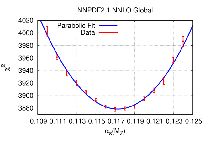
The values obtained for each value of are shown in Fig. 1; the total number of data points is [2], and at the minimum . The error bar shown on each point is the standard deviation determined using the bootstrap method as described in Ref. [1]. A parabolic fit leads to
| (1) |
where the statistical uncertainty corresponds to a shift by one from the minimum of the parabola, while the procedural uncertainty is propagated from the finite-size uncertainty on the values, and it is clearly completely negligible. The per degree of freedom of the parabolic fit shown in Fig. 1 is . This value remains unchanged if the outer two or four points are removed from the parabolic fit: this means that the behaviour of the curve shown is parabolic to within the accuracy of the individual points.
Equation (1) is the main result of this paper. It is interesting to compare this to the NLO result of Ref. [1], namely
| (2) |
which was obtained using exactly the same methodology, from PDFs in turn determined using the same methodology and the same data 111The number of datapoints for the NLO fit of Ref. [1] is [13]: the slightly lower number of datapoints in the NLO case is due to the fact that the kinematic cuts on charm structure function data must be more stringent at NLO in order to exclude data for which NNLO corrections are very large, as discussed in more detail in Ref. [2].; the value of the per data point at the minimum at NLO is also the same, namely . The result appears to be perturbatively quite stable. The small difference in statistical error between the NLO and NNLO fits indicates that the NLO fit quality deteriorates slightly faster when moving away from the minimum. However, this difference does not appear to be statistically significant: the gaussian uncertainty on the uncertainty is , which in our case, with and (the number of degrees of freedom of the parabolic fit) is .
The statistical uncertainty on the determination of Eq. (1) is very small when compared to the uncertainty on other existing determinations of : for example, the statistical uncertainty on the NNLO MSTW determination [3], which is also based on a PDF fit to a similar set of data, is twice as large. The size of the uncertainty on the MSTW08 result is significantly affected by the fact that a tolerance [14] criterion is used to obtain 68% confidence levels. This means that uncertainty ranges in parameter space are rescaled by an amount which is determined by requiring a reasonable behaviour of the distribution of best-fit results for the various parameters among the different experiments that enter the global fit, whose fluctuations may be significantly larger than expected on the basis of unrescaled uncertainties. It is thus important to establish whether such a rescaling is also necessary in our case.
We do this (as in Ref.[1]) using a variant of the method suggested in Ref. [15]. Namely, we determine that the distribution of results obtained from individual datasets follows a Gaussian distribution. A possible deviation from unity of the width of this distribution would then indicate the need for tolerance rescaling. Of course care should be taken that values obtained from individual experiments in a global fit are correlated by the underlying global fit; these correlations could in principle lead to spurious minima in the profile which would be absent if was fitted from that experiment only, and thus would be of no significance.
| Experiment | ||||||
|---|---|---|---|---|---|---|
| NMCpd | 0.1146 | 0.0105 | 0.0019 | 0.0107 | -0.25 | 0.5 |
| NMCp | 0.1150 | 0.0020 | 0.0003 | 0.0020 | -1.06 | 1.6 |
| BCDMS | 0.1158 | 0.0014 | 0.0002 | 0.0015 | -0.92 | 1.2 |
| HERA-I | 0.1199 | 0.0019 | 0.0002 | 0.0019 | 1.31 | 1.0 |
| ZEUS-H2 | 0.1231 | 0.0030 | 0.0002 | 0.0030 | 1.89 | 0.9 |
| NuTeV | 0.1177 | 0.0038 | 0.0004 | 0.0039 | 0.10 | 1.2 |
| CDFZRAP | 0.1205 | 0.0074 | 0.0033 | 0.0081 | 0.40 | 1.2 |
| CDFR2KT | 0.1225 | 0.0021 | 0.0003 | 0.0021 | 2.35 | 1.8 |
| D0R2CON | 0.1111 | 0.0028 | 0.0004 | 0.0029 | -2.10 | 0.5 |
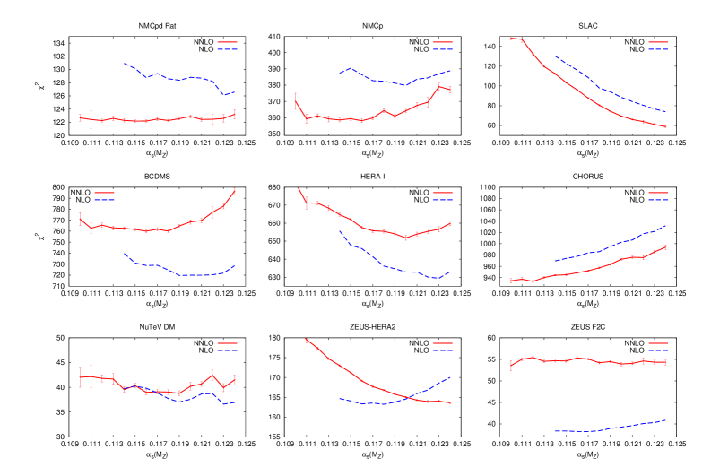
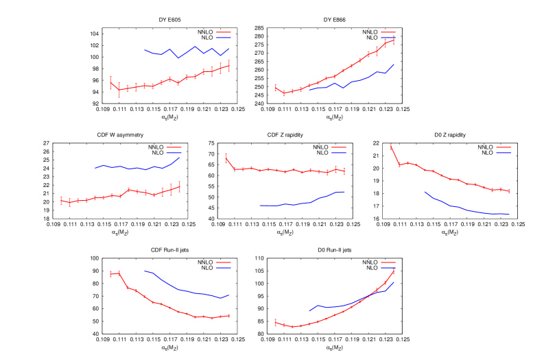
We have thus determined the profile of the contribution to the of the global fit from each experiment entering the global NNPDF2.1 NNLO determination: all profiles are displayed in Fig. 2, along with their NLO counterparts of Ref. [1]. We have then determined and its uncertainty from a parabolic fit to each profile. For each experiment whose parabola has a minimum in the fitted range we have determined the pull, defined as
| (3) |
where is the global best-fit value Eq. (1) and the uncertainty on it determined from the statistical and procedural uncertainties also of Eq. (1), while and are the corresponding values for the -th experiment. The best-fit value, statistical and procedural uncertainty for the -th experiment are determined by applying to the profile for the contribution of the -th experiment to the global fit exactly the same procedure used for the determination of the corresponding quantities in the global fit, and they are thus subject to the caveat that correlations with other experiments are neglected (for example, procedural uncertainties in each individual experiment will now have point-by-point correlation due to other experiments included in the global fit).
The best-fit values of , uncertainties and pulls are collected in Table 2, along with the of the parabolic fit to each individual profile.222Note that the definition of pull Eq. (3) is the same as in Eq. (3) of Ref.[1], however all pulls were incorrectly given in Table 3 of that reference with the opposite sign convention. Clearly for some datasets (such as NMCpd or CDFZRAP) the minimum is actually quite shallow, as apparent from Figure 2, and the uncertainty in Table 2 is correspondingly large: these data would not by themselves provide a determination of . However, note that here we are not determining the best-fit from each dataset, but rather studying the compatibility of different data sets within the global fit: from this point of view, data with a shallow minimum or no minimum are certainly compatible, and thus not problematic.
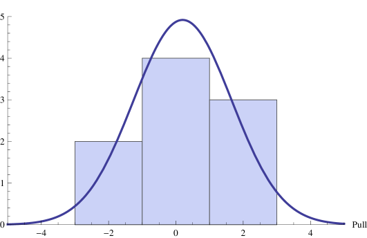
The pull distribution has mean and standard deviation
| (4) |
where the uncertainties on the mean and standard deviation are computed assuming that the population of nine pulls is extracted from a univariate Gaussian distribution. In Fig. 3 the histogram of the pull distribution is compared to a Gaussian normalized to the area under the histogram, and with mean and width given by Eq. (4). We conclude that the pull distribution is consistent, with either no need or minimal need for tolerance rescaling. Even if one were to rescale the statistical uncertainty on by the pull, one would end up with a statistical uncertainty of 0.0010 instead of 0.0007.
Having established that the estimate of the statistical uncertainty in our main result Eq. (1) is robust, we now turn to the issue of theoretical uncertainties. The main theoretical uncertainty comes from higher order QCD corrections. An indication of its size can be obtained by comparing results obtained at subsequent perturbative orders. Our NNLO and NLO results, Eqs. (1) and (2) respectively, differ by
| (5) |
This is likely to provide an upper bound to the uncertainty on the NNLO determination from higher order corrections. Hence, the perturbative stability of our result suggests that the higher order uncertainty on it is quite small.
A somewhat less crude estimate can be obtained using a method recently proposed in Ref. [16], based on the idea that a Bayesian estimate of the behaviour of unknown higher orders of a perturbative series can be obtained from the behaviour of the known orders. The 68% confidence level (i.e. one sigma) uncertainty due to higher order corrections to the -th order result
| (6) |
under the assumptions of the model in Ref. [16] is then given by
| (7) |
with the number of known perturbative coefficients.
In our case, the output value of in our analysis is not determined from the perturbative expansion of a single quantity, but rather from the expansion for all processes which enter the global PDF fit. However, we can obtain an estimate for its perturbative behaviour by letting
| (8) |
where is the result of our determination at a given perturbative order, while is some underlying input “true” value of the strong coupling. We then know the values of at NLO and NNLO, but we do not know the value of at LO, nor the input value . We obtain our estimate by varying both in a wide range: we take and and then we use Eq. (7), with Eq. (8) evaluated at NLO or NNLO, and take in each case the largest output value for as the input parameters are varied.
We then get
| (9) | |||
| (10) |
so that in particular the NNLO uncertainty is about half the shift between the NLO and NNLO values. Clearly, results depend significantly on the range of variation of : for example, if we restricted it to we would get and . We have chosen a very broad range in order to obtain a conservative estimate. A more careful assessment could be obtained by performing a similar analysis (or factorization and renormalization scale variation) for each of the processes which enters the global fit, and then combining the ensuing uncertainties, while the analysis given here should be viewed as a semi-quantitative way of putting on a firmer footing the expectation that the uncertainty on at a given order due to higher-order corrections should be a fraction of the shift of the best-fit value of from the previous to the given order.
We thus see that while at NLO theoretical uncertainties arising from higher perturbative orders are dominant over statistical uncertainties, at NNLO the two uncertainties are of similar size, and thus our determination of appears to remain quite accurate even when this uncertainty is included. Of the further sources of theoretical uncertainty, the largest is likely to be related to the treatment of heavy quarks, though such uncertainty is typically [17] smaller than that related to higher order corrections.
A sizable fraction of the data which are used for the NNPDF2.1 PDF determination comes from deep-inelastic scattering experiments. There is a widespread perception (see e.g. [18, 19]) that determinations based on deep-inelastic data lead to a value which is somewhat smaller than the global average. In Ref. [1], we have shown that in a DIS-only fit the BCDMS data (which have been long known [20] to favor a low ) have a minimum of the at rather low . However, this is no longer the case if the BCDMS data are included in a global fit along with Drell-Yan and jet data. We have traced this to the fact that at low DIS data and jet data pull the gluon in opposite directions, so the fit quality can be improved using DIS data only in a way which is forbidden when jet data are present. Similar results have been obtained in Refs. [21, 22], where it was further argued that this effect is stronger if the gluon parametrization is too restrictive, and it was in fact shown explicitly that within the MSTW fitting framework low NNLO best-fit values (similar or lower to the values obtained at NNLO in Ref. [4]) are obtained if either the gluon parametrization is more restrictive, or jet data are excluded from the fit. In Ref. [1] we found that in the NNPDF framework (where an extremely flexible PDF parametrization is used) the effect of the BCDMS data on the DIS fit remains moderate: though the BCDMS data favor a low value of , the DIS-only best fit is still , consistent with the global NLO best fit. However, the analysis of Ref. [1] is only performed at NLO, so one is immediately led to ask what happens at NNLO.
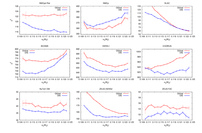
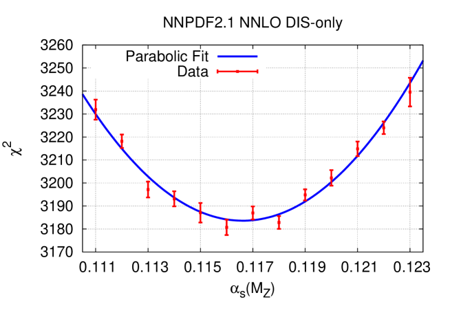
We have thus repeated our NNLO determination of , but now only including deep-inelastic scattering data in the computation of the . Starting with the NNPDF2.1 NNLO DIS-only fit of Ref. [2], we have generated replicas for all values of in the range from 0.110 to 0.124 in steps of 0.001. The values and finite-size uncertainties that we get are shown in Fig. 4, to be compared to Fig. 1 of the global fit; the number of data points now is [2], and at the minimum . A parabolic fit has a , and leads to
| (11) |
Note that the outer two points at have not been used, because the quality of the parabolic fit would considerably deteriorate. The profiles from individual datasets in the global and DIS-only fit are compared in Fig. 5.
Comparing our global and DIS-only determinations of Eqs. (1) and (11) we see that, like at NLO [1], also at NNLO the DIS-only value, though somewhat smaller than the global one, agrees with it within the (small) statistical uncertainty at the one sigma level. The pattern of profiles for individual experiments is also similar at NLO and NNLO: the BCDMS data have a minimum for much lower in the DIS only fit than in the global fit. Note however that the overall DIS-only best-fit value of Eq. (11) remains quite close to the global one, unlike in the MSTW08 case where the NNLO DIS-only value ends up being quite low (0.1139, to be compared to 0.1171 for the global fit) — perhaps because of our especially flexible PDF parametrization. In this respect, it is interesting to observe that MSTW find [21] that their DIS-only result depends strongly on whether the parametrization allows the gluon to become negative or not; in the NNPDF determination positivity is imposed at the level of physical observables, thus leading to a milder constraint on the PDF itself.
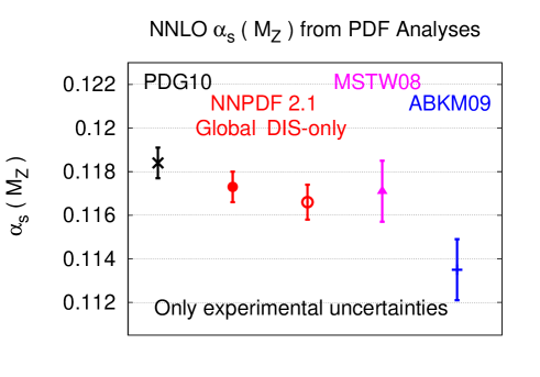
Our results for the NNLO determinations, both from the global data set and from DIS data only, are displayed graphically in Fig. 6, where they are also compared to the other recent NNLO ABKM09 [4] and MSTW08 [3] determinations. Our results are in good agreement with MSTW, but with smaller uncertainties. The ABKM result is rather lower, but it should be kept in mind that ABKM only use DIS data and a smaller set of fixed-target Drell-Yan data, with a parton parametrization which is more restrictive than the MSTW one, so it is subject to the caveats mentioned above and discussed in Ref. [21].
In summary, we have presented the most accurate available NNLO determination from a global parton fit. The greater statistical accuracy of our result in comparison to other available determinations of along with PDFs [3, 4] is due both to the use of the particularly flexible and reliable NNPDF approach to PDF parametrization and fitting, and to the use of a wide and up-to-date dataset (in particular the recent combined HERA data [23] which are not used in Refs. [3, 4]). The theoretical uncertainty on our determination is likely to be dominated by higher-order perturbative QCD corrections, and thus there is no reason why it should be different from any other analogous determination (such as Refs. [3, 4]). This uncertainty has not been determined accurately so far. However, the considerable perturbative stability we find, demonstrated by the moderate shift between our NLO and NNLO results, suggests that it might be smaller than hitherto expected: in particular, our estimate for it is less than half than that provided in Ref. [3]. It will be interesting to repeat this analysis once the very accurate data on standard candle processes from the LHC become available.
Acknowledgments
S.F. thanks A. Martin for communicating Ref. [22] prior to
publication, and G. Altarelli and R. Thorne for illuminating discussions.
J. R. is supported by a Marie Curie
Intra–European Fellowship of the European Community’s 7th Framework
Programme under contract number PIEF-GA-2010-272515.
M.U. is supported by the Bundesministerium für Bildung and Forschung (BmBF) of the Federal
Republic of Germany (project code 05H09PAE).
This work was
partly supported by the Spanish
MEC FIS2007-60350 grant.
We would like to acknowledge the use of the computing resources provided
by the Black Forest Grid Initiative in Freiburg and by the Edinburgh Compute
and Data Facility (ECDF) (http://www.ecdf.ed.ac.uk/). The ECDF is partially
supported by the eDIKT initiative (http://www.edikt.org.uk).
References
- [1] S. Lionetti et al., Phys. Lett. B701 (2011) 346, 1103.2369.
- [2] The NNPDF Collaboration, R.D. Ball et al., Nucl.Phys. B855 (2012) 153, 1107.2652.
- [3] A.D. Martin et al., Eur. Phys. J. C64 (2009) 653, 0905.3531.
- [4] S. Alekhin et al., Phys. Rev. D81 (2010) 014032, 0908.2766.
- [5] H.L. Lai et al., Phys.Rev. D82 (2010) 054021, 1004.4624.
- [6] LHC Higgs Cross Section Working Group, S. Dittmaier et al., (2011), 1101.0593.
- [7] The NNPDF collaboration, L. Del Debbio et al., JHEP 03 (2005) 080, hep-ph/0501067.
- [8] The NNPDF collaboration, L. Del Debbio et al., JHEP 03 (2007) 039, hep-ph/0701127.
- [9] The NNPDF Collaboration, R.D. Ball et al., Nucl. Phys. B809 (2009) 1, 0808.1231.
- [10] The NNPDF collaboration, R.D. Ball et al., Nucl. Phys. B823 (2009) 195, 0906.1958.
- [11] The NNPDF collaboration, R.D. Ball et al., Nucl. Phys. B838 (2010) 136, 1002.4407.
- [12] The NNPDF Collaboration, R.D. Ball et al., (2011), 1108.1758.
- [13] The NNPDF Collaboration, R.D. Ball et al., Nucl. Phys. B849 (2011) 296, 1101.1300.
- [14] J. Pumplin et al., Phys.Rev. D65 (2001) 014013, hep-ph/0101032.
- [15] J. Pumplin, Phys. Rev. D81 (2010) 074010, 0909.0268.
- [16] M. Cacciari and N. Houdeau, JHEP 1109 (2011) 039, 1105.5152.
- [17] R.D. Ball and S. Forte, Phys.Lett. B358 (1995) 365, hep-ph/9506233.
- [18] S. Bethke, Eur. Phys. J. C64 (2009) 689, 0908.1135.
- [19] S. Bethke et al., (2011), 1110.0016.
- [20] M. Virchaux and A. Milsztajn, Phys. Lett. B274 (1992) 221.
- [21] R. Thorne and G. Watt, JHEP 1108 (2011) 100, 1106.5789.
- [22] A.D. Martin et al., in MSTW analyses, in: S. Bethke et al, ”Workshop on Precision Measurements of alphas”, arXiv:1110.0016, 2011.
- [23] H1 and ZEUS Collaboration, F. Aaron et al., JHEP 1001 (2010) 109, 0911.0884.