The Generalized A* Architecture

Abstract

We consider the problem of computing a lightest derivation of a global structure using a set of weighted rules. A large variety of inference problems in AI can be formulated in this framework. We generalize A* search and heuristics derived from abstractions to a broad class of lightest derivation problems. We also describe a new algorithm that searches for lightest derivations using a hierarchy of abstractions. Our generalization of A* gives a new algorithm for searching AND/OR graphs in a bottom-up fashion.

We discuss how the algorithms described here provide a general architecture for addressing the pipeline problem — the problem of passing information back and forth between various stages of processing in a perceptual system. We consider examples in computer vision and natural language processing. We apply the hierarchical search algorithm to the problem of estimating the boundaries of convex objects in grayscale images and compare it to other search methods. A second set of experiments demonstrate the use of a new compositional model for finding salient curves in images.

1 Introduction

We consider a class of problems defined by a set of weighted rules for composing structures into larger structures. The goal in such problems is to find a lightest (least cost) derivation of a global structure derivable with the given rules. A large variety of classical inference problems in AI can be expressed within this framework. For example the global structure might be a parse tree, a match of a deformable object model to an image, or an assignment of values to variables in a Markov random field.

We define a lightest derivation problem in terms of a set of statements, a set of weighted rules for deriving statements using other statements and a special goal statement. In each case we are looking for the lightest derivation of the goal statement. We usually express a lightest derivation problem using rule “schemas” that implicitly represent a very large set of rules in terms of a small number of rules with variables. Lightest derivation problems are formally equivalent to search in AND/OR graphs (?), but we find that our formulation is more natural for the applications we are interested in.

One of the goals of this research is the construction of algorithms for global optimization across many levels of processing in a perceptual system. As described below our algorithms can be used to integrate multiple stages of a processing pipeline into a single global optimization problem that can be solved efficiently.

Dynamic programming is a fundamental technique for designing efficient inference algorithms. Good examples are the Viterbi algorithm for hidden Markov models (?) and chart parsing methods for stochastic context free grammars (?). The algorithms described here can be used to speed up the solution of problems normally solved using dynamic programming. We demonstrate this for a specific problem, where the goal is to estimate the boundary of a convex object in a cluttered image. In a second set of experiments we show how our algorithms can be used to find salient curves in images. We describe a new model for salient curves based on a compositional rule that enforces long range shape constraints. This leads to a problem that is too large to be solved using classical dynamic programming methods.

The algorithms we consider are all related to Dijkstra’s shortest paths algorithm (DSP) (?) and A* search (?). Both DSP and A* can be used to find a shortest path in a cyclic graph. They use a priority queue to define an order in which nodes are expanded and have a worst case running time of $O(M\log N)$ where $N$ is the number of nodes in the graph and $M$ is the number of edges. In DSP and A* the expansion of a node $v$ involves generating all nodes $u$ such that there is an edge from $v$ to $u$. The only difference between the two methods is that A* uses a heuristic function to avoid expanding non-promising nodes.

Knuth gave a generalization of DSP that can be used to solve a lightest derivation problem with cyclic rules (?). We call this Knuth’s lightest derivation algorithm (KLD). In analogy to Dijkstra’s algorithm, KLD uses a priority queue to define an order in which statements are expanded. Here the expansion of a statement $v$ involves generating all conclusions that can be derived in a single step using $v$ and other statements already expanded. As long as each rule has a bounded number of antecedents KLD also has a worst case running time of $O(M\log N)$ where $N$ is the number of statements in the problem and $M$ is the number of rules. Nilsson’s AO* algorithm (?) can also be used to solve lightest derivation problems. Although AO* can use a heuristic function, it is not a true generalization of A* — it does not use a priority queue, only handles acyclic rules, and can require $O(MN)$ time even when applied to a shortest path problem. In particular, AO* and its variants use a backward chaining technique that starts at the goal and repeatedly refines subgoals, while A* is a forward chaining algorithm.

? (?) described an A* parsing algorithm that is similar to KLD but can use a heuristic function. One of our contributions is a generalization of this algorithm to arbitrary lightest derivation problems. We call this algorithm A* lightest derivation (A*LD). The method is forward chaining, uses a priority queue to control the order in which statements are expanded, handles cyclic rules and has a worst case running time of $O(M\log N)$ for problems where each rule has a small number of antecedents. A*LD can be seen as a true generalization of A* to lightest derivation problems. For a lightest derivation problem that comes from a shortest path problem A*LD is identical to A*.

Of course the running times seen in practice are often not well predicted by worst case analysis. This is specially true for problems that are very large and defined implicitly. For example, we can use dynamic programming to solve a shortest path problem in an acyclic graph in $O(M)$ time. This is better than the $O(M\log N)$ bound for DSP, but for implicit graphs DSP can be much more efficient since it expands nodes in a best-first order. When searching for a shortest path from a source to a goal, DSP will only expand nodes $v$ with $d(v)\leq w^{*}$. Here $d(v)$ is the length of a shortest path from the source to $v$, and $w^{*}$ is the length of a shortest path from the source to the goal. In the case of A* with a monotone and admissible heuristic function, $h(v)$, it is possible to obtain a similar bound when searching implicit graphs. A* will only expand nodes $v$ with $d(v)+h(v)\leq w^{*}$.

The running time of KLD and A*LD can be expressed in a similar way. When solving a lightest derivation problem, KLD will only expand statements $v$ with $d(v)\leq w^{*}$. Here $d(v)$ is the weight of a lightest derivation for $v$, and $w^{*}$ is the weight of a lightest derivation of the goal statement. Furthermore, A*LD will only expand statements $v$ with $d(v)+h(v)\leq w^{*}$. Here the heuristic function, $h(v)$, gives an estimate of the additional weight necessary for deriving the goal statement using a derivation of $v$. The heuristic values used by A*LD are analogous to the distance from a node to the goal in a graph search problem (the notion used by A*). We note that these heuristic values are significantly different from the ones used by AO*. In the case of AO* the heuristic function, $h(v)$, would estimate the weight of a lightest derivation for $v$.

An important difference between A*LD and AO* is that A*LD computes derivations in a bottom-up fashion, while AO* uses a top-down approach. Each method has advantages, depending on the type of problem being solved. For example, a classical problem in computer vision involves grouping pixels into long and smooth curves. We can formulate the problem in terms of finding smooth curves between pairs of pixels that are far apart. For an image with $n$ pixels there are $\Omega(n^{2})$ such pairs. A straight forward implementation of a top-down algorithm would start by considering these $\Omega(n^{2})$ possibilities. A bottom-up algorithm would start with $O(n)$ pairs of nearby pixels. In this case we expect that a bottom-up grouping method would be more efficient than a top-down method.

The classical AO* algorithm requires the set of rules to be acyclic. ? (?) extended the method to handle cyclic rules. Another top-down algorithm that can handle cyclic rules is described by ? (?). ? (?) described a search algorithm for problems where the optimal solutions themselves can be cyclic. The algorithms described in this paper can handle problems with cyclic rules but require that the optimal solutions be acyclic. We also note that AO* can handle rules with non-superior weight functions (as defined in Section 3) while KLD requires superior weight functions. A*LD replaces this requirement by a requirement on the heuristic function.

A well known method for defining heuristics for A* is to consider an abstract or relaxed search problem. For example, consider the problem of solving a Rubik’s cube in a small number of moves. Suppose we ignore the edge and center pieces and solve only the corners. This is an example of a problem abstraction. The number of moves necessary to put the corners in a good configuration is a lower bound on the number of moves necessary to solve the original problem. There are fewer corner configurations than there are full configurations and that makes it easier to solve the abstract problem. In general, shortest paths to the goal in an abstract problem can be used to define an admissible and monotone heuristic function for solving the original problem with A*.

Here we show that abstractions can also be used to define heuristic functions for A*LD. In a lightest derivation problem the notion of a shortest path to the goal is replaced by the notion of a lightest context, where a context for a statement $v$ is a derivation of the goal with a “hole” that can be filled in by a derivation of $v$. The computation of lightest abstract contexts is itself a lightest derivation problem.

Abstractions are related to problem relaxations defined by ? (?). While abstractions often lead to small problems that are solved through search, relaxations can lead to problems that still have a large state space but may be simple enough to be solved in closed form. The definition of abstractions that we use for lightest derivation problems includes relaxations as a special case.

Another contribution of our work is a hierarchical search method that we call HA*LD. This algorithm can effectively use a hierarchy of abstractions to solve a lightest derivation problem. The algorithm is novel even in the case of classical search (shortest paths) problem. HA*LD searches for lightest derivations and contexts at every level of abstraction simultaneously. More specifically, each level of abstraction has its own set of statements and rules. The search for lightest derivations and contexts at each level is controlled by a single priority queue. To understand the running time of HA*LD, let $w^{*}$ be the weight of a lightest derivation of the goal in the original (not abstracted) problem. For a statement $v$ in the abstraction hierarchy let $d(v)$ be the weight of a lightest derivation for $v$ at its level of abstraction. Let $h(v)$ be the weight of a lightest context for the abstraction of $v$ (defined at one level above $v$ in the hierarchy). Let $K$ be the total number of statements in the hierarchy with $d(v)+h(v)\leq w^{*}$. HAL*D expands at most $2K$ statements before solving the original problem. The factor of two comes from the fact that the algorithm computes both derivations and contexts at each level of abstraction.

Previous algorithms that use abstractions for solving search problems include methods based on pattern databases (?, ?, ?), Hierarchical A* (HA*, HIDA*) (?, ?) and coarse-to-fine dynamic programming (CFDP) (?). Pattern databases have made it possible to compute solutions to impressively large search problems. These methods construct a lookup table of shortest paths from a node to the goal at all abstract states. In practice the approach is limited to tables that remain fixed over different problem instances, or relatively small tables if the heuristic must be recomputed for each instance. For example, for the Rubik’s cube we can precompute the number of moves necessary to solve every corner configuration. This table can be used to define a heuristic function when solving any full configuration of the Rubik’s cube. Both HA* and HIDA* use a hierarchy of abstractions and can avoid searching over all nodes at any level of the hierarchy. On the other hand, in directed graphs these methods may still expand abstract nodes with arbitrarily large heuristic values. It is also not clear how to generalize HA* and HIDA* to lightest derivation problems that have rules with more than one antecedent. Finally, CFDP is related to AO* in that it repeatedly solves ever more refined problems using dynamic programming. This leads to a worst case running time of $O(NM)$. We will discuss the relationships between HA*LD and these other hierarchical methods in more detail in Section 8.

We note that both A* search and related algorithms have been previously used to solve a number of problems that are not classical state space search problems. This includes the traveling salesman problem (?), planning (?), multiple sequence alignment (?), combinatorial problems on graphs (?) and parsing using context-free-grammars (?). The work by ? (?) uses a hierarchy of state-space abstractions for real-time search.

1.1 The Pipeline Problem

A major problem in artificial intelligence is the integration of multiple processing stages to form a complete perceptual system. We call this the pipeline problem. In general we have a concatenation of systems where each stage feeds information to the next. In vision, for example, we might have an edge detector feeding information to a boundary finding system, which in turn feeds information to an object recognition system.

Because of computational constraints and the need to build modules with clean interfaces pipelines often make hard decisions at module boundaries. For example, an edge detector typically constructs a Boolean array that indicates weather or not an edge was detected at each image location. But there is general recognition that the presence of an edge at a certain location can depend on the context around it. People often see edges at places where the image gradient is small if, at higher cognitive level, it is clear that there is actually an object boundary at that location. Speech recognition systems try to address this problem by returning n-best lists, but these may or may not contain the actual utterance. We would like the speech recognition system to be able to take high-level information into account and avoid the hard decision of exactly what strings to output in its n-best list.

A processing pipeline can be specified by describing each of its stages in terms of rules for constructing structures using structures produced from a previous stage. In a vision system one stage could have rules for grouping edges into smooth curves while the next stage could have rules for grouping smooth curves into objects. In this case we can construct a single lightest derivation problem representing the entire system. Moreover, a hierarchical set of abstractions can be applied to the entire pipeline. By using HA*LD to compute lightest derivations a complete scene interpretation derived at one level of abstraction guides all processing stages at a more concrete level. This provides a mechanism that enables coarse high-level processing to guide low-level computation. We believe that this is an important property for implementing efficient perceptual pipelines that avoid making hard decisions between processing stages.

We note that the formulation of a complete computer vision system as a lightest derivation problem is related to the work by ? (?), ? (?) and ? (?). In these papers image understanding is posed as a parsing problem, where the goal is to explain the image in terms of a set of objects that are formed by the (possibly recursive) composition of generic parts. ? (?) use data driven MCMC to compute “optimal” parses while ? (?) and ? (?) use a bottom-up algorithm for building compositions in a greedy fashion. Neither of these methods are guaranteed to compute an optimal scene interpretation. We hope that HA*LD will provide a more principled computational technique for solving large parsing problems defined by compositional models.

1.2 Overview

We begin by formally defining lightest derivation problems in Section 2. That section also discusses dynamic programming and the relationship between lightest derivation problems and AND/OR graphs. In Section 3 we describe Knuth’s lightest derivation algorithm. In Section 4 we describe A*LD and prove its correctness. Section 5 shows how abstractions can be used to define mechanically constructed heuristic functions for A*LD. We describe HA*LD in Section 6 and discuss its use in solving the pipeline problem in Section 7. Section 8 discusses the relationship between HA*LD and other hierarchical search methods. In Sections 9 and 10 we present some experimental results. We conclude in Section 11.

2 Lightest Derivation Problems

Let $\Sigma$ be a set of statements and $R$ be a set of inference rules of the following form,

$A_{1}=w_{1}$

$\vdots$

$A_{n}=w_{n}$

$C=g(w_{1},\ldots,w_{n})$

Here the antecedents $A_{i}$ and the conclusion $C$ are statements in $\Sigma$, the weights $w_{i}$ are non-negative real valued variables and $g$ is a non-negative real valued weight function. For a rule with no antecedents the function $g$ is simply a non-negative real value. Throughout the paper we also use $A_{1},\ldots,A_{n}\rightarrow_{g}C$ to denote an inference rule of this type.

A derivation of $C$ is a finite tree rooted at a rule $A_{1},\ldots,A_{n}\rightarrow_{g}C$ with $n$ children, where the $i$-th child is a derivation of $A_{i}$. The leaves of this tree are rules with no antecedents. Every derivation has a weight that is the value obtained by recursive application of the functions $g$ along the derivation tree. Figure 1 illustrates a derivation tree.

Figure 1: A derivation of $C$ is a tree of rules rooted at a rule $r$ with conclusion $C$. The children of the root are derivations of the antecedents in $r$. The leafs of the tree are rules with no antecedents.

Intuitively a rule $A_{1},\ldots,A_{n}\rightarrow_{g}C$ says that if we can derive the antecedents $A_{i}$ with weights $w_{i}$ then we can derive the conclusion $C$ with weight $g(w_{1},\ldots,w_{n})$. The problem we are interested in is to compute a lightest derivation of a special goal statement.

All of the algorithms discussed in this paper assume that the weight functions $g$ associated with a lightest derivation problem are non-decreasing in each variable. This is a fundamental property ensuring that lightest derivations have an optimal substructure property. In this case lightest derivations can be constructed from other lightest derivations.

To facilitate the runtime analysis of algorithms we assume that every rule has a small number of antecedents. We use $N$ to denote the number of statements in a lightest derivation problem, while $M$ denotes the number of rules. For most of the problems we are interested in $N$ and $M$ are very large but the problem can be implicitly defined in a compact way, by using a small number of rules with variables as in the examples below. We also assume that $N\leq M$ since statements that are not in the conclusion of some rule are clearly not derivable and can be ignored.

2.1 Dynamic Programming

We say that a set of rules is acyclic if there is an ordering $O$ of the statements in $\Sigma$ such that for any rule with conclusion $C$ the antecedents are statements that come before $C$ in the ordering. Dynamic programming can be used to solve a lightest derivation problem if the functions $g$ in each rule are non-decreasing and the set of rules is acyclic. In this case lightest derivations can be computed sequentially in terms of an acyclic ordering $O$. At the $i$-th step a lightest derivation of the $i$-th statement is obtained by minimizing over all rules that can be used to derive that statement. This method takes $O(M)$ time to compute a lightest derivation for each statement in $\Sigma$.

We note that for cyclic rules it is sometimes possible to compute lightest derivations by taking multiple passes over the statements. We also note that some authors would refer to Dijkstra’s algorithm (and KLD) as a dynamic programming method. In this paper we only use the term when referring to algorithms that compute lightest derivations in a fixed order that is independent of the solutions computed along the way (this includes recursive implementations that use memoization).

2.2 Examples

Rules for computing shortest paths from a single source in a weighted graph are shown in Figure 2.2. We assume that we are given a weighted graph $G=(V,E)$, where $w_{xy}$ is a non-negative weight for each edge $(x,y)\in E$ and $s$ is a distinguished start node. The first rule states that there is a path of weight zero to the start node $s$. The second set of rules state that if there is a path to a node $x$ we can extend that path with an edge from $x$ to $y$ to obtain an appropriately weighted path to a node $y$. There is a rule of this type for each edge in the graph. A lightest derivation of $\text{\emph{path}}(x)$ corresponds to shortest path from $s$ to $x$. Note that for general graphs these rules can be cyclic. Figure 3 illustrates a graph and two different derivations of $\text{\emph{path}}(b)$ using the rules just described. These corresponds to two different paths from $s$ to $b$.

(1)

$\text{\emph{path}}(s)=0$

(2) for each $(x,y)\in E$,

$\text{\emph{path}}(x)=w$

$\text{\emph{path}}(y)=w+w_{xy}$

Figure 2: Rules for computing shortest paths in a graph.

Figure 3: A graph with two highlighted paths from $s$ to $b$ and the corresponding derivations using rules from Figure 2.2.

Rules for chart parsing are shown in Figure 2.2. We assume that we are given a weighted context free grammar in Chomsky normal form (?), i.e., a weighted set of productions of the form $X\rightarrow s$ and $X\rightarrow YZ$ where $X$, $Y$ and $Z$ are nonterminal symbols and $s$ is a terminal symbol. The input string is given by a sequence of terminals $(s_{1},\ldots,s_{n})$. The first set of rules state that if the grammar contains a production $X\rightarrow s_{i}$ then there is a phrase of type $X$ generating the $i$-th entry of the input with weight $w(X\rightarrow s_{i})$. The second set of rules state that if the grammar contains a production $X\rightarrow YZ$ and there is a phrase of type $Y$ from $i$ to $j$ and a phrase of type $Z$ from $j$ to $k$ then there is an, appropriately weighted, phrase of type $X$ from $i$ to $k$. Let $S$ be the start symbol of the grammar. The goal of parsing is to find a lightest derivation of $\text{\emph{phrase}}(S,1,n+1)$. These rules are acyclic because when phrases are composed together they form longer phrases.

(1) for each production $X\rightarrow s_{i}$,

$\text{\emph{phrase}}(X,i,i+1)=w(X\rightarrow s_{i})$

(2) for each production $X\rightarrow YZ$ and $1\leq i<j<k\leq n+1$,

$\text{\emph{phrase}}(Y,i,j)=w_{1}$

$\text{\emph{phrase}}(Z,j,k)=w_{2}$

$\text{\emph{phrase}}(X,i,k)=w_{1}+w_{2}+w(X\rightarrow YZ)$

Figure 4: Rules for parsing with a context free grammar.

2.3 AND/OR Graphs

Lightest derivation problems are closely related to AND/OR graphs. Let $\Sigma$ and $R$ be a set of statements and rules defining a lightest derivation problem. To convert the problem to an AND/OR graph representation we can build a graph with a disjunction node for each statement in $\Sigma$ and a conjunction node for each rule in $R$. There is an edge from each statement to each rule deriving that statement, and an edge from each rule to its antecedents. The leaves of the AND/OR graph are rules with no antecedents. Now derivations of a statement using rules in $R$ can be represented by solutions rooted at that statement in the corresponding AND/OR graph. Conversely, it is also possible to represent any AND/OR graph search problem as a lightest derivation problem. In this case we can view each node in the graph as a statement in $\Sigma$ and build an appropriate set of rules $R$.

3 Knuth’s Lightest Derivation

? (?) described a generalization of Dijkstra’s shortest paths algorithm that we call Knuth’s lightest derivation (KLD). Knuth’s algorithm can be used to solve a large class of lightest derivation problems. The algorithm allows the rules to be cyclic but requires that the weight functions associated with each rule be non-decreasing and superior. Specifically we require the following two properties on the weight function $g$ in each rule,

non-decreasing: $$\mbox{if}\;w^{\prime}_{i}\geq w_{i}\;\mbox{then}\;g(w_{1},\ldots,w^{\prime}_{i},\ldots,w_{n})\geq g(w_{1},\ldots,w_{i},\ldots,w_{n})$$

superior: $$g(w_{1},\ldots,w_{n})\geq w_{i}$$

For example,

$$\begin{array}[]{l}g(x_{1},\ldots,x_{n})=x_{1}+\cdots+x_{n}\\ g(x_{1},\ldots,x_{n})=\max(x_{1},\ldots,x_{n})\end{array}$$

are both non-decreasing and superior functions.

Knuth’s algorithm computes lightest derivations in non-decreasing weight order. Since we are only interested in a lightest derivation of a special goal statement we can often stop the algorithm before computing the lightest derivation of every statement.

A weight assignment is an expression of the form $(B=w)$ where $B$ is a statement in $\Sigma$ and $w$ is a non-negative real value. We say that the weight assignment $(B=w)$ is derivable if there is a derivation of $B$ with weight $w$. For any set of rules $R$, statement $B$, and weight $w$ we write $R\vdash(B=w)$ if the rules in $R$ can be used to derive $(B=w)$. Let $\ell(B,R)$ be the infimum of the set of weights derivable for $B$,

$$\ell(B,R)=\inf\{w:\;R\vdash(B=w)\}.$$

Given a set of rules $R$ and a statement $\text{\emph{goal}}\in\Sigma$ we are interested in computing a derivation of goal with weight $\ell(\text{\emph{goal}},R)$.

We define a bottom-up logic programming language in which we can easily express the algorithms we wish to discuss throughout the rest of the paper. Each algorithm is defined by a set of rules with priorities. We encode the priority of a rule by writing it along the line separating the antecedents and the conclusion as follows,

$A_{1}=w_{1}$

$\vdots$

$A_{n}=w_{n}$

$p(w_{1},\ldots,w_{n})$

$C=g(w_{1},\ldots,w_{n})$

We call a rule of this form a prioritized rule. The execution of a set of prioritized rules $P$ is defined by the procedure in Figure 5. The procedure keeps track of a set ${\cal S}$ and a priority queue ${\cal Q}$ of weight assignments of the form $(B=w)$. Initially ${\cal S}$ is empty and ${\cal Q}$ contains weight assignments defined by rules with no antecedents at the priorities given by those rules. We iteratively remove the lowest priority assignment $(B=w)$ from ${\cal Q}$. If $B$ already has an assigned weight in ${\cal S}$ then the new assignment is ignored. Otherwise we add the new assignment to ${\cal S}$ and “expand it” — every assignment derivable from $(B=w)$ and other assignments already in ${\cal S}$ using some rule in $P$ is added to ${\cal Q}$ at the priority specified by the rule. The procedure stops when the queue is empty.

• ${\cal S}\mathrel{\leftarrow}\emptyset$

• Initialize ${\cal Q}$ with assignments defined by rules with no antecedents at their priorities

• while ${\cal Q}$ is not empty

• Remove the lowest priority element $(B=w)$ from ${\cal Q}$

• if $B$ has no assigned weight in ${\cal S}$

• ${\cal S}\mathrel{\leftarrow}{\cal S}\cup\{(B=w)\}$

• Insert assignments derivable from $(B=w)$ and other assignments in ${\cal S}$ using some rule in $P$ into ${\cal Q}$ at the priority specified by the rule

• return ${\cal S}$

Figure 5: Running a set of prioritized rules.

The result of executing a set of prioritized rules is a set of weight assignments. Moreover, the procedure can implicitly keep track of derivations by remembering which assignments were used to derive an item that is inserted in the queue.

Lemma 1.

The execution of a finite set of prioritized rules $P$ derives every statement that is derivable with rules in $P$.

Proof.

Each rule causes at most one item to be inserted in the queue. Thus eventually ${\cal Q}$ is empty and the algorithm terminates. When ${\cal Q}$ is empty every statement derivable by a single rule using antecedents with weight in ${\cal S}$ already has a weight in ${\cal S}$. This implies that every derivable statement has a weight in ${\cal S}$. ∎

Now we are ready to define Knuth’s lightest derivation algorithm. The algorithm is easily described in terms of prioritized rules.

Definition 1 (Knuth’s lightest derivation).

Let $R$ be a finite set of non-decreasing and superior rules. Define a set of prioritized rules ${\cal K}(R)$ by setting the priority of each rule in $R$ to be the weight of the conclusion. KLD is given by the execution of ${\cal K}(R)$.

We can show that while running ${\cal K}(R)$, if $(B=w)$ is added to ${\cal S}$ then $w=\ell(B,R)$. This means that all assignments in ${\cal S}$ represent lightest derivations. We can also show that assignments are inserted into ${\cal S}$ in non-decreasing weight order. If we stop the algorithm as soon as we insert a weight assignment for goal into ${\cal S}$ we will expand all statements $B$ such that $\ell(B,R)<\ell(\text{\emph{goal}},R)$ and some statements $B$ such that $\ell(B,R)=\ell(\text{\emph{goal}},R)$. These properties follow from a more general result described in the next section.

3.1 Implementation

The algorithm in Figure 5 can be implemented to run in $O(M\log N)$ time, where $N$ and $M$ refer to the size of the problem defined by the prioritized rules $P$.

In practice the set of prioritized rules $P$ is often specified implicitly, in terms of a small number of rules with variables. In this case the problem of executing $P$ is closely related to the work on logical algorithms described by ? (?).

The main difficulty in devising an efficient implementation of the procedure in Figure 5 is in step 7. In that step we need to find weight assignments in ${\cal S}$ that can be combined with $(B=w)$ to derive new weight assignments. The logical algorithms work shows how a set of inference rules with variables can be transformed into a new set of rules, such that every rule has at most two antecedents and is in a particularly simple form. Moreover, this transformation does not increase the number of rules too much. Once the rules are transformed their execution can be implemented efficiently using a hashtable to represent ${\cal S}$, a heap to represent ${\cal Q}$ and indexing tables that allow us to perform step 7 quickly.

Consider the second set of rules for parsing in Figure 2.2. These can be represented by a single rule with variables. Moreover the rule has two antecedents. When executing the parsing rules we keep track of a table mapping a value for $j$ to statements $\text{\emph{phrase}}(Y,i,j)$ that have a weight in ${\cal S}$. Using this table we can quickly find statements that have a weight in ${\cal S}$ and can be combined with a statement of the form $\text{\emph{phrase}}(Z,j,k)$. Similarly we keep track of a table mapping a value for $j$ to statements $\text{\emph{phrase}}(Z,j,k)$ that have a weight in ${\cal S}$. The second table lets us quickly find statements that can be combined with a statement of the form $\text{\emph{phrase}}(Y,i,j)$. We refer the reader to (?) for more details.

4 A* Lightest Derivation

Our A* lightest derivation algorithm (A*LD) is a generalization of A* search to lightest derivation problems that subsumes A* parsing. The algorithm is similar to KLD but it can use a heuristic function to speed up computation. Consider a lightest derivation problem with rules $R$ and goal statement goal. Knuth’s algorithm will expand any statement $B$ such that $\ell(B,R)<\ell(\text{\emph{goal}},R)$. By using a heuristic function A*LD can avoid expanding statements that have light derivations but are not part of a light derivation of goal.

Let $R$ be a set of rules with statements in $\Sigma$, and $h$ be a heuristic function assigning a weight to each statement. Here $h(B)$ is an estimate of the additional weight required to derive goal using a derivation of $B$. We note that in the case of a shortest path problem this weight is exactly the distance from a node to the goal. The value $\ell(B,R)+h(B)$ provides a figure of merit for each statement $B$. The A* lightest derivation algorithm expands statements in order of their figure of merit.

We say that a heuristic function is monotone if for every rule $A_{1},\ldots,A_{n}\rightarrow_{g}C$ in $R$ and derivable weight assignments $(A_{i}=w_{i})$ we have,

$$w_{i}+h(A_{i})\leq g(w_{1},\ldots,w_{n})+h(C).$$ (1)

This definition agrees with the standard notion of a monotone heuristic function for rules that come from a shortest path problem. We can show that if $h$ is monotone and $h(\text{\emph{goal}})=0$ then $h$ is admissible under an appropriate notion of admissibility. For the correctness of A*LD, however, it is only required that $h$ be monotone and that $h(\text{\emph{goal}})$ be finite. In this case monotonicity implies that the heuristic value of every statement $C$ that appears in a derivation of goal is finite. Below we assume that $h(C)$ is finite for every statement. If $h(C)$ is not finite we can ignore $C$ and every rule that derives $C$.

Definition 2 (A* lightest derivation).

Let $R$ be a finite set of non-decreasing rules and $h$ be a monotone heuristic function for $R$. Define a set of prioritized rules ${\cal A}(R)$ by setting the priority of each rule in $R$ to be the weight of the conclusion plus the heuristic value, $g(w_{1},\ldots,w_{n})+h(C)$. A*LD is given by the execution of ${\cal A}(R)$.

Now we show that the execution of ${\cal A}(R)$ correctly computes lightest derivations and that it expands statements in order of their figure of merit values.

Theorem 2.

During the execution of ${\cal A}(R)$, if $(B=w)\in{\cal S}$ then $w=\ell(B,R)$.

Proof.

The proof is by induction on the size of ${\cal S}$. The statement is trivial when ${\cal S}=\emptyset$. Suppose the statement was true right before the algorithm removed $(B=w_{b})$ from ${\cal Q}$ and added it to ${\cal S}$. The fact that $(B=w_{b})\in{\cal Q}$ implies that the weight assignment is derivable and thus $w_{b}\geq\ell(B,R)$.

Suppose $T$ is a derivation of $B$ with weight $w_{b}^{\prime}<w_{b}$. Consider the moment right before the algorithm removed $(B=w_{b})$ from ${\cal Q}$ and added it to ${\cal S}$. Let $A_{1},\ldots,A_{n}\rightarrow_{g}C$ be a rule in $T$ such that the antecedents $A_{i}$ have a weight in ${\cal S}$ while the conclusion $C$ does not. Let $w_{c}=g(\ell(A_{1},R),\ldots,\ell(A_{n},R))$. By the induction hypothesis the weight of $A_{i}$ in ${\cal S}$ is $\ell(A_{i},R)$. Thus $(C=w_{c})\in{\cal Q}$ at priority $w_{c}+h(C)$. Let $w_{c}^{\prime}$ be the weight that $T$ assigns to $C$. Since $g$ is non-decreasing we know $w_{c}\leq w_{c}^{\prime}$. Since $h$ is monotone $w_{c}^{\prime}+h(C)\leq w_{b}^{\prime}+h(B)$. This follows by using the monotonicity condition along the path from $C$ to $B$ in $T$. Now note that $w_{c}+h(C)<w_{b}+h(B)$ which in turn implies that $(B=w_{b})$ is not the weight assignment in ${\cal Q}$ with minimum priority. ∎

Theorem 3.

During the execution of ${\cal A}(R)$ statements are expanded in order of the figure of merit value $\ell(B,R)+h(B)$.

Proof.

First we show that the minimum priority of ${\cal Q}$ does not decrease throughout the execution of the algorithm. Suppose $(B=w)$ is an element in ${\cal Q}$ with minimum priority. Removing $(B=w)$ from ${\cal Q}$ does not decrease the minimum priority. Now suppose we add $(B=w)$ to ${\cal S}$ and insert assignments derivable from $(B=w)$ into ${\cal Q}$. Since $h$ is monotone the priority of every assignment derivable from $(B=w)$ is at least the priority of $(B=w)$.

A weight assignment $(B=w)$ is expanded when it is removed from ${\cal Q}$ and added to ${\cal S}$. By the last theorem $w=\ell(B,R)$ and by the definition of ${\cal A}(R)$ this weight assignment was queued at priority $\ell(B,R)+h(B)$. Since we removed $(B=w)$ from ${\cal Q}$ this must be the minimum priority in the queue. The minimum priority does not decrease over time so we must expand statements in order of their figure of merit value. ∎

If we have accurate heuristic functions A*LD can be much more efficient than KLD. Consider a situation where we have a perfect heuristic function. That is, suppose $h(B)$ is exactly the additional weight required to derive goal using a derivation of $B$. Now the figure of merit $\ell(B,R)+h(B)$ equals the weight of a lightest derivation of goal that uses $B$. In this case A*LD will derive goal before expanding any statements that are not part of a lightest derivation of goal.

The correctness KLD follows from the correctness of A*LD. For a set of non-decreasing and superior rules we can consider the trivial heuristic function $h(B)=0$. The fact that the rules are superior imply that this heuristic is monotone. The theorems above imply that Knuth’s algorithm correctly computes lightest derivations and expands statements in order of their lightest derivable weights.

5 Heuristics Derived from Abstractions

Here we consider the case of additive rules — rules where the weight of the conclusion is the sum of the weights of the antecedents plus a non-negative value $v$ called the weight of the rule. We denote such a rule by $A_{1},\ldots,A_{n}\rightarrow_{v}C$. The weight of a derivation using additive rules is the sum of the weights of the rules that appear in the derivation tree.

A context for a statement $B$ is a finite tree of rules such that if we add a derivation of $B$ to the tree we get a derivation of goal. Intuitively a context for $B$ is a derivation of goal with a “hole” that can be filled in by a derivation of $B$ (see Figure 6).

Figure 6: A derivation of goal defines contexts for the statements that appear in the derivation tree. Note how a context for $C$ together with a rule $A_{1},A_{2},A_{3}\rightarrow C$ and derivations of $A_{1}$ and $A_{2}$ define a context for $A_{3}$.

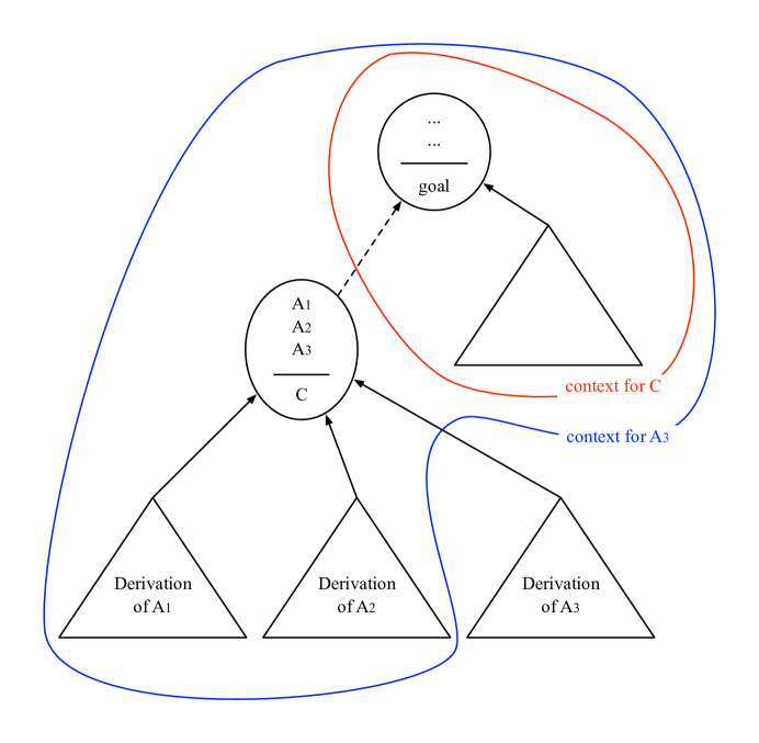
For additive rules, each context has a weight that is the sum of weights of the rules in it. Let $R$ be a set of additive rules with statements in $\Sigma$. For $B\in\Sigma$ we define $\ell(\text{\emph{context}}(B),R)$ to be the weight of a lightest context for $B$. The value $\ell(B,R)+\ell(\text{\emph{context}}(B),R)$ is the weight of a lightest derivation of goal that uses $B$.

Contexts can be derived using rules in $R$ together with context rules $c(R)$ defined as follows. First, $goal$ has an empty context with weight zero. This is captured by a rule with no antecedents $\rightarrow_{0}\text{\emph{context}}(\text{\emph{goal}})$. For each rule $A_{1},\ldots,A_{n}\rightarrow_{v}C$ in $R$ we put $n$ rules in $c(R)$. These rules capture the notion that a context for $C$ and derivations of $A_{j}$ for $j\neq i$ define a context for $A_{i}$,

$$\text{\emph{context}}(C),A_{1},\ldots,A_{i-1},A_{i+1},\ldots,A_{n}\rightarrow_{v}\text{\emph{context}}(A_{i}).$$

Figure 6 illustrates how a context for $C$ together with derivations of $A_{1}$ and $A_{2}$ and a rule $A_{1},A_{2},A_{3}\rightarrow C$ define a context for $A_{3}$.

We say that a heuristic function $h$ is admissible if $h(B)\leq\ell(\text{\emph{context}}(B),R)$. Admissible heuristic functions never over-estimate the weight of deriving goal using a derivation of a particular statement. The heuristic function is perfect if $h(B)=\ell(\text{\emph{context}}(B),R)$. Now we show how to obtain admissible and monotone heuristic functions from abstractions.

5.1 Abstractions

Let $(\Sigma,R)$ be a lightest derivation problem with statements $\Sigma$ and rules $R$. An abstraction of $(\Sigma,R)$ is given by a problem $(\Sigma^{\prime},R^{\prime})$ and a map $\text{\emph{abs}}\!:\!\Sigma\!\rightarrow\!\Sigma^{\prime}$, such that for every rule $A_{1},\ldots,A_{n}\rightarrow_{v}C$ in $R$ there is a rule $abs(A_{1}),\ldots,abs(A_{n})\rightarrow_{v^{\prime}}\text{\emph{abs}}(C)$ in $R^{\prime}$ with $v^{\prime}\leq v$. Below we show how an abstraction can be used to define a monotone and admissible heuristic function for the original problem.

We usually think of abs as defining a coarsening of $\Sigma$ by mapping several statements into the same abstract statement. For example, for a parser abs might map a lexicalized nonterminal $NP_{\mathrm{house}}$ to the nonlexicalized nonterminal $NP$. In this case the abstraction defines a smaller problem on the abstract statements. Abstractions can often be defined in a mechanical way by starting with a map abs from $\Sigma$ into some set of abstract statements $\Sigma^{\prime}$. We can then “project” the rules in $R$ from $\Sigma$ into $\Sigma^{\prime}$ using abs to get a set of abstract rules. Typically several rules in $R$ will map to the same abstract rule. We only need to keep one copy of each abstract rule, with a weight that is a lower bound on the weight of the concrete rules mapping into it.

Every derivation in $(\Sigma,R)$ maps to an abstract derivation so we have $\ell(\text{\emph{abs}}(C),R^{\prime})\leq\ell(C,R)$. If we let the goal of the abstract problem be $\text{\emph{abs}}(\text{\emph{goal}})$ then every context in $(\Sigma,R)$ maps to an abstract context and we see that $\ell(\text{\emph{context}}(\text{\emph{abs}}(C)),R^{\prime})\leq\ell(\text{\emph{context}}(C),R)$. This means that lightest abstract context weights form an admissible heuristic function,

$$h(C)=\ell(\text{\emph{context}}(\text{\emph{abs}}(C)),R^{\prime}).$$

Now we show that this heuristic function is also monotone.

Consider a rule $A_{1},\ldots,A_{n}\rightarrow_{v}C$ in $R$ and let $(A_{i}=w_{i})$ be weight assignments derivable using $R$. In this case there is a rule $\text{\emph{abs}}(A_{1}),\ldots,\text{\emph{abs}}(A_{n})\rightarrow_{v^{\prime}}\text{\emph{abs}}(C)$ in $R^{\prime}$ where $v^{\prime}\leq v$ and $(abs(A_{i})=w_{i}^{\prime})$ is derivable using $R^{\prime}$ where $w_{i}^{\prime}\leq w_{i}$. By definition of contexts (in the abstract problem) we have,

$$\ell(\text{\emph{context}}(\text{\emph{abs}}(A_{i})),R^{\prime})\leq v^{\prime}+\sum_{j\neq i}w_{j}^{\prime}+\ell(\text{\emph{context}}(\text{\emph{abs}}(C)),R^{\prime}).$$

Since $v^{\prime}\leq v$ and $w_{j}^{\prime}\leq w_{j}$ we have,

$$\ell(\text{\emph{context}}(\text{\emph{abs}}(A_{i})),R^{\prime})\leq v+\sum_{j\neq i}w_{j}+\ell(\text{\emph{context}}(\text{\emph{abs}}(C)),R^{\prime}).$$

Plugging in the heuristic function $h$ from above and adding $w_{i}$ to both sides,

$$w_{i}+h(A_{i})\leq v+\sum_{j}w_{j}+h(C),$$

which is exactly the monotonicity condition in equation (1) for an additive rule.

If the abstract problem defined by $(\Sigma^{\prime},R^{\prime})$ is relatively small we can efficiently compute lightest context weights for every statement in $\Sigma^{\prime}$ using dynamic programming or KLD. We can store these weights in a “pattern database” (a lookup table) to serve as a heuristic function for solving the concrete problem using A*LD. This heuristic may be able to stop A*LD from exploring a lot of non-promising structures. This is exactly the approach that was used by ? (?) and ? (?) for solving very large search problems. The results in this section show that pattern databases can be used in the more general setting of lightest derivations problems. The experiments in Section 10 demonstrate the technique in a specific application.

6 Hierarchical A* Lightest Derivation

The main disadvantage of using pattern databases is that we have to precompute context weights for every abstract statement. This can often take a lot of time and space. Here we define a hierarchical algorithm, HA*LD, that searches for lightest derivations and contexts in an entire abstraction hierarchy simultaneously. This algorithm can often solve the most concrete problem without fully computing context weights at any level of abstraction.

At each level of abstraction the behavior HA*LD is similar to the behavior of A*LD when using an abstraction-derived heuristic function. The hierarchical algorithm queues derivations of a statement $C$ at a priority that depends on a lightest abstract context for $C$. But now abstract contexts are not computed in advance. Instead, abstract contexts are computed at the same time we are computing derivations. Until we have an abstract context for $C$, derivations of $C$ are “stalled”. This is captured by the addition of $\text{\emph{context}}(\text{\emph{abs}}(C))$ as an antecedent to each rule that derives $C$.

We define an abstraction hierarchy with $m$ levels to be a sequence of lightest derivation problems with additive rules $(\Sigma_{k},R_{k})$ for $0\leq k\leq m-1$ with a single abstraction function abs. For $0\leq k<m-1$ the abstraction function maps $\Sigma_{k}$ onto $\Sigma_{k+1}$. We require that $(\Sigma_{k+1},R_{k+1})$ be an abstraction of $(\Sigma_{k},R_{k})$ as defined in the previous section: if $A_{1},\ldots,A_{n}\rightarrow_{v}C$ is in $R_{k}$ then there exists a rule $\text{\emph{abs}}(A_{1}),\ldots,\text{\emph{abs}}(A_{n})\rightarrow_{v^{\prime}}\text{\emph{abs}}(C)$ in $R_{k+1}$ with $v^{\prime}\leq v$. The hierarchical algorithm computes lightest derivations of statements in $\Sigma_{k}$ using contexts from $\Sigma_{k+1}$ to define heuristic values. We extend abs so that it maps $\Sigma_{m-1}$ to a most abstract set of statements $\Sigma_{m}$ containing a single element $\bot$. Since abs is onto we have $|\Sigma_{k}|\geq|\Sigma_{k+1}|$. That is, the number of statements decrease as we go up the abstraction hierarchy. We denote by $\text{\emph{abs}}_{k}$ the abstraction function from $\Sigma_{0}$ to $\Sigma_{k}$ obtained by composing abs with itself $k$ times.

We are interested in computing a lightest derivation of a goal statement $\text{\emph{goal}}\in\Sigma_{0}$. Let $\text{\emph{goal}}_{k}=\text{\emph{abs}}_{k}(\text{\emph{goal}})$ be the goal at each level of abstraction. The hierarchical algorithm is defined by the set of prioritized rules ${\cal H}$ in Figure 7. Rules labeled UP compute derivations of statements at one level of abstraction using context weights from the level above to define priorities. Rules labeled BASE and DOWN compute contexts in one level of abstraction using derivation weights at the same level to define priorities. The rules labeled START1 and START2 start the inference by handling the most abstract level.

START1:

$0$

$\bot=0$

START2:

$0$

$\text{\emph{context}}(\bot)=0$

BASE:

$\text{\emph{goal}}_{k}=w$

$w$

$\text{\emph{context}}(\text{\emph{goal}}_{k})=0$

UP:

$\text{\emph{context}}(\text{\emph{abs}}(C))=w_{c}$

$A_{1}=w_{1}$

$\hskip 4.30554pt\vdots$

$A_{n}=w_{n}$

$v+w_{1}+\cdots+w_{n}+w_{c}$

$C=v+w_{1}+\cdots+w_{n}$

DOWN:

$\text{\emph{context}}(C)=w_{c}$

$A_{1}=w_{1}$

$\hskip 4.30554pt\vdots$

$A_{n}=w_{n}$

$v+w_{c}+w_{1}+\cdots+w_{n}$

$\text{\emph{context}}(A_{i})=v+w_{c}+w_{1}+\cdots+w_{n}-w_{i}$

Figure 7: Prioritized rules ${\cal H}$ defining HA*LD. BASE rules are defined for $0\leq k\leq m-1$. UP and DOWN rules are defined for each rule $A_{1},\ldots,A_{n}\rightarrow_{v}C\in R_{k}$ with $0\leq k\leq m-1$.

The execution of ${\cal H}$ starts by computing a derivation and context for $\bot$ with START1 and START2. It continues by deriving statements in $\Sigma_{m-1}$ using UP rules. Once the lightest derivation of $\text{\emph{goal}}_{m-1}$ is found the algorithm derives a context for $\text{\emph{goal}}_{m-1}$ with a BASE rule and starts computing contexts for other statements in $\Sigma_{m-1}$ using DOWN rules. In general HA*LD interleaves the computation of derivations and contexts at each level of abstraction since the execution of ${\cal H}$ uses a single priority queue.

Note that no computation happens at a given level of abstraction until a lightest derivation of the goal has been found at the level above. This means that the structure of the abstraction hierarchy can be defined dynamically. For example, as in the CFDP algorithm, we could define the set of statements at each level of abstraction by refining the statements that appear in a lightest derivation of the goal at the level above. Here we assume a static abstraction hierarchy.

For each statement $C\in\Sigma_{k}$ with $0\leq k\leq m-1$ we use $\ell(C)$ to denote the weight of a lightest derivation for $C$ using $R_{k}$ while $\ell(\text{\emph{context}}(C))$ denotes the weight of a lightest context for $C$ using $R_{k}$. For the most abstract level we define $\ell(\bot)=\ell(\text{\emph{context}}(\bot))=0$.

Below we show that HA*LD correctly computes lightest derivations and lightest contexts at every level of abstraction. Moreover, the order in which derivations and contexts are expanded is controlled by a heuristic function defined as follows. For $C\in\Sigma_{k}$ with $0\leq k\leq m-1$ define a heuristic value for $C$ using contexts at the level above and a heuristic value for $\text{\emph{context}}(C)$ using derivations at the same level,

$$\begin{array}[]{l}h(C)=\ell(\text{\emph{context}}(\text{\emph{abs}}(C))),\\ h(\text{\emph{context}}(C))=\ell(C).\end{array}$$

For the most abstract level we define $h(\bot)=h(\text{\emph{context}}(\bot))=0$. Let a generalized statement $\Phi$ be either an element of $\Sigma_{k}$ for $0\leq k\leq m$ or an expression of the form $\text{\emph{context}}(C)$ for $C\in\Sigma_{k}$. We define an intrinsic priority for $\Phi$ as follows,

$$p(\Phi)=\ell(\Phi)+h(\Phi).$$

For $C\in\Sigma_{k}$, we have that $p(\text{\emph{context}}(C))$ is the weight of a lightest derivation of $\text{\emph{goal}}_{k}$ that uses $C$, while $p(C)$ is a lower bound on this weight.

The results from Sections 4 and 5 cannot be used directly to show the correctness of HA*LD. This is because the rules in Figure 7 generate heuristic values at the same time they generate derivations that depend on those heuristic values. Intuitively we must show that during the execution of the prioritized rules ${\cal H}$, each heuristic value is available at an appropriate point in time. The next lemma shows that the rules in ${\cal H}$ satisfy a monotonicity property with respect to the intrinsic priority of generalized statements. Theorem 5 proves the correctness of the hierarchical algorithm.

Lemma 4 (Monotonicity).

For each rule $\Phi_{1},\ldots,\Phi_{m}\rightarrow\Psi$ in the hierarchical algorithm, if the weight of each antecedent $\Phi_{i}$ is $\ell(\Phi_{i})$ and the weight of the conclusion is $\alpha$ then

• the priority of the rule is $\alpha+h(\Psi)$.

• $\alpha+h(\Psi)\geq p(\Phi_{i})$.

Proof.

For the rules START1 and START2 the result follows from the fact that the rules have no antecedents and $h(\bot)=h(\text{\emph{context}}(\bot))=0$.

Consider a rule labeled BASE with $w=\ell(\text{\emph{goal}}_{k})$. To see (a) note that $\alpha$ is always zero and the priority of the rule is $w=h(\text{\emph{context}}(\text{\emph{goal}}_{k}))$. For (b) we note that $p(\text{\emph{goal}}_{k})=\ell(\text{\emph{goal}}_{k})$ which equals the priority of the rule.

Now consider a rule labeled UP with $w_{c}=\ell(\text{\emph{context}}(\text{\emph{abs}}(C)))$ and $w_{i}=\ell(A_{i})$ for all $i$. For part (a) note how the priority of the rule is $\alpha+w_{c}$ and $h(C)=w_{c}$. For part (b) consider the first antecedent of the rule. We have $h(\text{\emph{context}}(\text{\emph{abs}}(C)))=\ell(\text{\emph{abs}}(C))\leq\ell(C)\leq\alpha$, and $p(\text{\emph{context}}(\text{\emph{abs}}(C)))=w_{c}+h(\text{\emph{context}}(\text{\emph{abs}}(C)))\leq\alpha+w_{c}$. Now consider an antecedent $A_{i}$. If $\text{\emph{abs}}(A_{i})=\bot$ then $p(A_{i})=w_{i}\leq\alpha+w_{c}$. If $\text{\emph{abs}}(A_{i})\neq\bot$ then we can show that $h(A_{i})=\ell(\text{\emph{context}}(\text{\emph{abs}}(A_{i})))\leq w_{c}+\alpha-w_{i}$. This implies that $p(A_{i})=w_{i}+h(A_{i})\leq\alpha+w_{c}$.

Finally consider a rule labeled DOWN with $w_{c}=\ell(\text{\emph{context}}(C))$ and $w_{j}=\ell(A_{j})$ for all $j$. For part (a) note that the priority of the rule is $\alpha+w_{i}$ and $h(\text{\emph{context}}(A_{i}))=w_{i}$. For part (b) consider the first antecedent of the rule. We have $h(\text{\emph{context}}(C))=\ell(C)\leq v+\sum_{j}w_{j}$ and we see that $p(\text{\emph{context}}(C))=w_{c}+h(C)\leq\alpha+w_{i}$. Now consider an antecedent $A_{j}$. If $\text{\emph{abs}}(A_{j})=\bot$ then $h(A_{j})=0$ and $p(A_{j})=w_{j}\leq\alpha+w_{i}$. If $\text{\emph{abs}}(A_{j})\neq\bot$ we can show that $h(A_{j})\leq\alpha+w_{i}-w_{j}$. Hence $p(A_{j})=w_{j}+h(A_{j})\leq\alpha+w_{i}$. ∎

Theorem 5.

The execution of ${\cal H}$ maintains the following invariants.

1. If $(\Phi=w)\in{\cal S}$ then $w=\ell(\Phi)$.

2. If $(\Phi=w)\in{\cal Q}$ then it has priority $w+h(\Phi)$.

3. If $p(\Phi)<p({\cal Q})$ then $(\Phi=\ell(\Phi))\in{\cal S}$

Here $p({\cal Q})$ denotes the smallest priority in ${\cal Q}$.

Proof.

In the initial state of the algorithm ${\cal S}$ is empty and ${\cal Q}$ contains only $(\bot=0)$ and $(\text{\emph{context}}(\bot)=0)$ at priority $0$. For the initial state invariant 1 is true since ${\cal S}$ is empty; invariant 2 follows from the definition of $h(\bot)$ and $h(\text{\emph{context}}(\bot))$; and invariant 3 follows from the fact that $p({\cal Q})=0$ and $p(\Phi)\geq 0$ for all $\Phi$. Let ${\cal S}$ and ${\cal Q}$ denote the state of the algorithm immediately prior to an iteration of the while loop in Figure 5 and suppose the invariants are true. Let ${\cal S}^{\prime}$ and ${\cal Q}^{\prime}$ denote the state of the algorithm after the iteration.

We will first prove invariant 1 for ${\cal S}^{\prime}$. Let $(\Phi=w)$ be the element removed from ${\cal Q}$ in this iteration. By the soundness of the rules we have $w\geq\ell(\Phi)$. If $w=\ell(\Phi)$ then clearly invariant 1 holds for ${\cal S}^{\prime}$. If $w>\ell(\Phi)$ invariant 2 implies that $p({\cal Q})=w+h(\Phi)>\ell(\Phi)+h(\Phi)$ and by invariant 3 we know that ${\cal S}$ contains $(\Phi=\ell(\Phi))$. In this case ${\cal S}^{\prime}={\cal S}$.

Invariant 2 for ${\cal Q}^{\prime}$ follows from invariant 2 for ${\cal Q}$, invariant 1 for ${\cal S}^{\prime}$, and part (a) of the monotonicity lemma.

Finally, we consider invariant 3 for ${\cal S}^{\prime}$ and ${\cal Q}^{\prime}$. The proof is by reverse induction on the abstraction level of $\Phi$. We say that $\Phi$ has level $k$ if $\Phi\in\Sigma_{k}$ or $\Phi$ is of the form $\text{\emph{context}}(C)$ with $C\in\Sigma_{k}$. In the reverse induction, the base case considers $\Phi$ at level $m$. Initially the algorithm inserts $(\bot=0)$ and $(\text{\emph{context}}(\bot)=0)$ in the queue with priority $0$. If $p({\cal Q}^{\prime})>0$ then ${\cal S}^{\prime}$ must contain $(\bot=0)$ and $(\text{\emph{context}}(\bot)=0)$. Hence invariant 3 holds for ${\cal S}^{\prime}$ and ${\cal Q}^{\prime}$ with $\Phi$ at level $m$.

Now we assume that invariant 3 holds for ${\cal S}^{\prime}$ and ${\cal Q}^{\prime}$ with $\Phi$ at levels greater than $k$ and consider level $k$. We first consider statements $C\in\Sigma_{k}$. Since the rules $R_{k}$ are additive, every statement $C$ derivable with $R_{k}$ has a lightest derivation (a derivation with weight $\ell(C)$). This follows from the correctness of Knuth’s algorithm. Moreover, for additive rules, subtrees of lightest derivations are also lightest derivations. We show by structural induction that for any lightest derivation with conclusion $C$ such that $p(C)<p({\cal Q}^{\prime})$ we have $(C=\ell(C))\in{\cal S}^{\prime}$. Consider a lightest derivation in $R_{k}$ with conclusion $C$ such that $p(C)<p({\cal Q}^{\prime})$. The final rule in this derivation $A_{1},\ldots,A_{n}\rightarrow_{v}C$ corresponds to an UP rule where we add an antecedent for $\text{\emph{context}}(\text{\emph{abs}}(C))$. By part (b) of the monotonicity lemma all the antecedents of this UP rule have intrinsic priority less than $p({\cal Q}^{\prime})$. By the induction hypothesis on lightest derivations we have $(A_{i}=\ell(A_{i}))\in{\cal S}^{\prime}$. Since invariant 3 holds for statements at levels greater than $k$ we have $(\text{\emph{context}}(\text{\emph{abs}}(C))=\ell(\text{\emph{context}}(\text{\emph{abs}}(C))))\in{\cal S}^{\prime}$. This implies that at some point the UP rule was used to derive $(C=\ell(C))$ at priority $p(C)$. But $p(C)<p({\cal Q}^{\prime})$ and hence this item must have been removed from the queue. Therefore ${\cal S}^{\prime}$ must contain $(C=w)$ for some $w$ and, by invariant 1, $w=\ell(C)$.

Now we consider $\Phi$ of the form $\text{\emph{context}}(C)$ with $C\in\Sigma_{k}$. As before we see that $c(R_{k})$ is additive and thus every statement derivable with $c(R_{k})$ has a lightest derivation and subtrees of lightest derivations are lightest derivations themselves. We prove by structural induction that for any lightest derivation $T$ with conclusion $\text{\emph{context}}(C)$ such that $p(\text{\emph{context}}(C))<p({\cal Q}^{\prime})$ we have $(\text{\emph{context}}(C)=\ell(\text{\emph{context}}(C)))\in{\cal S}^{\prime}$. Suppose the last rule of $T$ is of the form,

$$\text{\emph{context}}(C),A_{1},\ldots,A_{i-1},A_{i+1},\ldots,A_{n}\rightarrow_{v}\text{\emph{context}}(A_{i}).$$

This rule corresponds to a DOWN rule where we add an antecedent for $A_{i}$. By part (b) of the monotonicity lemma all the antecedents of this DOWN rule have intrinsic priority less than $p({\cal Q}^{\prime})$. By invariant 3 for statements in $\Sigma_{k}$ and by the induction hypothesis on lightest derivations using $c(R_{k})$, all antecedents of the DOWN rule have their lightest weight in ${\cal S}^{\prime}$. So at some point $(\text{\emph{context}}(A_{i})=\ell(\text{\emph{context}}(A_{i})))$ was derived at priority $p(A_{i})$. Now $p(A_{i})<p({\cal Q}^{\prime})$ implies the item was removed from the queue and, by invariant 1, we have $(\text{\emph{context}}(A_{i})=\ell(\text{\emph{context}}(A_{i})))\in{\cal S}^{\prime}$.

Now suppose the last (and only) rule in $T$ is $\rightarrow_{0}\text{\emph{context}}(\text{\emph{goal}}_{k})$. This rule corresponds to a BASE rule where we add $\text{\emph{goal}}_{k}$ as an antecedent. Note that $p(\text{\emph{goal}}_{k})=\ell(\text{\emph{goal}}_{k})=p(\text{\emph{context}}(\text{\emph{goal}}_{k}))$ and hence $p(\text{\emph{goal}}_{k})<p({\cal Q}^{\prime})$. By invariant 3 for statements in $\Sigma_{k}$ we have $(\text{\emph{goal}}_{k}=\ell(\text{\emph{goal}}_{k}))$ in ${\cal S}^{\prime}$ and at some point the BASE rule was used to queue $(\text{\emph{context}}(\text{\emph{goal}}_{k})=\ell(\text{\emph{context}}(\text{\emph{goal}}_{k})))$ at priority $p(\text{\emph{context}}(\text{\emph{goal}}_{k}))$. As in the previous cases $p(\text{\emph{context}}(\text{\emph{goal}}_{k}))<p({\cal Q}^{\prime})$ implies $(\text{\emph{context}}(\text{\emph{goal}}_{k})=\ell(\text{\emph{context}}(\text{\emph{goal}}_{k})))\in{\cal S}^{\prime}$. ∎

The last theorem implies that generalized statements $\Phi$ are expanded in order of their intrinsic priority. Let $K$ be the number of statements $C$ in the entire abstraction hierarchy with $p(C)\leq p(\text{\emph{goal}})=\ell(\text{\emph{goal}})$. For every statement $C$ we have that $p(C)\leq p(\text{\emph{context}}(C))$. We conclude that HA*LD expands at most $2K$ generalized statements before computing a lightest derivation of goal.

6.1 Example

Now we consider the execution of HA*LD in a specific example. The example illustrates how HA*LD interleaves the computation of structures at different levels of abstraction. Consider the following abstraction hierarchy with 2 levels.

$$\Sigma_{0}=\{X_{1},\ldots,X_{n},Y_{1},\ldots,Y_{n},Z_{1},\ldots,Z_{n},\text{\emph{goal}}_{0}\},\;\;\;\Sigma_{1}=\{X,Y,Z,\text{\emph{goal}}_{1}\},$$

$$R_{0}=\left\{\begin{array}[]{l}\rightarrow_{i}X_{i},\\ \rightarrow_{i}Y_{i},\\ X_{i},Y_{j}\rightarrow_{i*j}\text{\emph{goal}}_{0},\\ X_{i},Y_{i}\rightarrow_{5}Z_{i},\\ Z_{i}\rightarrow_{i}\text{\emph{goal}}_{0},\end{array}\right\},\;\;\;R_{1}=\left\{\begin{array}[]{l}\rightarrow_{1}X,\\ \rightarrow_{1}Y,\\ X,Y\rightarrow_{1}\text{\emph{goal}}_{1},\\ X,Y\rightarrow_{5}Z,\\ Z\rightarrow_{1}\text{\emph{goal}}_{1},\end{array}\right\},$$

with $\text{\emph{abs}}(X_{i})=X$, $\text{\emph{abs}}(Y_{i})=Y$, $\text{\emph{abs}}(Z_{i})=Z$ and $\text{\emph{abs}}(goal_{0})=goal_{1}$.

1. Initially ${\cal S}=\emptyset$ and ${\cal Q}=\{(\bot=0)\text{ and }(\text{\emph{context}}(\bot)=0)\text{ at priority 0}\}$.

2. When $(\bot=0)$ comes off the queue it gets put in ${\cal S}$ but nothing else happens.

3. When $(\text{\emph{context}}(\bot)=0)$ comes off the queue it gets put in ${\cal S}$. Now statements in $\Sigma_{1}$ have an abstract context in ${\cal S}$. This causes UP rules that come from rules in $R_{1}$ with no antecedents to “fire”, putting $(X=1)$ and $(Y=1)$ in ${\cal Q}$ at priority 1.

4. When $(X=1)$ and $(Y=1)$ come off the queue they get put in ${\cal S}$, causing two UP rules to fire, putting $(\text{\emph{goal}}_{1}=3)$ at priority 3 and $(Z=7)$ at priority 7 in the queue.

5. We have,

   $${\cal S}=\{(\bot=0),\;(\text{\emph{context}}(\bot)=0),\;(X=1),\;(Y=1)\}$$

   $${\cal Q}=\{(\text{\emph{goal}}_{1}=3)\text{ at priority 3},\;(Z=7)\text{ at priority 7}\}$$

6. At this point $(\text{\emph{goal}}_{1}=3)$ comes off the queue and goes into in ${\cal S}$. A BASE rule fires putting $(\text{\emph{context}}(\text{\emph{goal}}_{1})=0)$ in the queue at priority 3.

7. $(\text{\emph{context}}(\text{\emph{goal}}_{1})=0)$ comes off the queue. This is the base case for contexts in $\Sigma_{1}$. Two DOWN rules use $(\text{\emph{context}}(\text{\emph{goal}}_{1})=0)$, $(X=1)$ and $(Y=1)$ to put $(\text{\emph{context}}(X)=2)$ and $(\text{\emph{context}}(Y)=2)$ in ${\cal Q}$ at priority 3.

8. $(\text{\emph{context}}(X)=2)$ comes off the queue and gets put in ${\cal S}$. Now we have an abstract context for each $X_{i}\in\Sigma_{0}$, so UP rules to put $(X_{i}=i)$ in ${\cal Q}$ at priority $i+2$.

9. Now $(\text{\emph{context}}(Y)=2)$ comes off the queue and goes into ${\cal S}$. As in the previous step UP rules put $(Y_{i}=i)$ in ${\cal Q}$ at priority $i+2$.

10. We have,

    $${\cal S} = \{(\bot=0),\;(\text{\emph{context}}(\bot)=0),\;(X=1),\;(Y=1),\;(\text{\emph{goal}}_{1}=3),\;$$

    $$(\text{\emph{context}}(\text{\emph{goal}}_{1})=0),\;(\text{\emph{context}}(X)=2),\;(\text{\emph{context}}(Y)=2)\}$$

    $${\cal Q}=\{(X_{i}=i)\text{ and }(Y_{i}=i)\text{ at priority $i+2$ for $1\leq i\leq n$},\;(Z=7)\text{ at priority 7}\}$$

11. Next both $(X_{1}=1)$ and $(Y_{1}=1)$ will come off the queue and go into ${\cal S}$. This causes an UP rule to put $(\text{\emph{goal}}_{0}=3)$ in the queue at priority 3.

12. $(\text{\emph{goal}}_{0}=3)$ comes off the queue and goes into ${\cal S}$. The algorithm can stop now since we have a derivation of the most concrete goal.

Note how HA*LD terminates before fully computing abstract derivations and contexts. In particular $(Z=7)$ is in ${\cal Q}$ but $Z$ was never expanded. Moreover $\text{\emph{context}}(Z)$ is not even in the queue. If we keep running the algorithm it would eventually derive $\text{\emph{context}}(Z)$, and that would allow the $Z_{i}$ to be derived.

7 The Perception Pipeline

Figure 8 shows a hypothetical run of the hierarchical algorithm for a processing pipeline of a vision system. In this system weighted statements about edges are used to derive weighted statements about contours which provide input to later stages ultimately resulting in statements about recognized objects.

It is well known that the subjective presence of edges at a particular image location can depend on the context in which a given image patch appears. This can be interpreted in the perception pipeline by stating that higher level processes — those later in the pipeline — influence low-level interpretations. This kind of influence happens naturally in a lightest derivation problem. For example, the lightest derivation of a complete scene analysis might require the presence of an edge that is not locally apparent. By implementing the whole system as a single lightest derivation problem we avoid the need to make hard decisions between stages of the pipeline.

Figure 8: A vision system with several levels of processing. Forward arrows represent the normal flow of information from one stage of processing to the next. Backward arrows represent the computation of contexts. Downward arrows represent the influence of contexts.

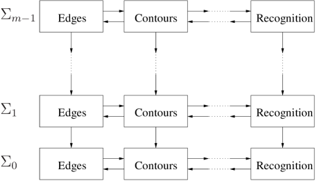
The influence of late pipeline stages in guiding earlier stages is pronounced if we use HA*LD to compute lightest derivations. In this case the influence is apparent not only in the structure of the optimal solution but also in the flow of information across different stages of processing. In HA*LD a complete interpretation derived at one level of abstraction guides all processing stages at a more concrete level. Structures derived at late stages of the pipeline guide earlier stages through abstract context weights. This allows the early processing stages to concentrate computational efforts in constructing structures that will likely be part of the globally optimal solution.

While we have emphasized the use of admissible heuristics, we note that the A* architecture, including HA*LD, can also be used with inadmissible heuristic functions (of course this would break our optimality guarantees). Inadmissible heuristics are important because admissible heuristics tend to force the first few stages of a processing pipeline to generate too many derivations. As derivations are composed their weights increase and this causes a large number of derivations to be generated at the first few stages of processing before the first derivation reaches the end of the pipeline. Inadmissible heuristics can produce behavior similar to beam search — derivations generated in the first stage of the pipeline can flow through the whole pipeline quickly. A natural way to construct inadmissible heuristics is to simply “scale-up” an admissible heuristic such as the ones obtained from abstractions. It is then possible to construct a hierarchical algorithm where inadmissible heuristics obtained from one level of abstraction are used to guide search at the level below.

8 Other Hierarchical Methods

In this section we compare HA*LD to other hierarchical search methods.

8.1 Coarse-to-Fine Dynamic Programming

HA*LD is related to the coarse-to-fine dynamic programming (CFDP) method described by ? (?). To understand the relationship consider the problem of finding the shortest path from $s$ to $t$ in a trellis graph like the one shown in Figure 9(a). Here we have $k$ columns of $n$ nodes and every node in one column is connected to a constant number of nodes in the next column. Standard dynamic programming can be used to find the shortest path in $O(kn)$ time. Both CFDP and HA*LD can often find the shortest path much faster. On the other hand the worst case behavior of these algorithms is very different as we describe below, with CFDP taking significantly more time than HA*LD.

The CFDP algorithm works by coarsening the graph, grouping nodes in each column into a small number of supernodes as illustrated in Figure 9(b). The weight of an edge between two supernodes $A$ and $B$ is the minimum weight between nodes $a\in A$ and $b\in B$. The algorithm starts by using dynamic programming to find the shortest path $P$ from $s$ to $t$ in the coarse graph, this is shown in bold in Figure 9(b). The supernodes along $P$ are partitioned to define a finer graph as shown in Figure 9(c) and the procedure repeated. Eventually the shortest path $P$ will only go through supernodes of size one, corresponding to a path in the original graph. At this point we know that $P$ must be a shortest path from $s$ to $t$ in the original graph. In the best case the optimal path in each iteration will be a refinement of the optimal path from the previous iteration. This would result in $O(\log n)$ shortest paths computations, each in fairly coarse graphs. On the other hand, in the worst case CFDP will take $\Omega(n)$ iterations to refine the whole graph, and many of the iterations will involve finding shortest paths in large graphs. In this case CFDP takes $\Omega(kn^{2})$ time which is much worst than the standard dynamic programming approach.

Now suppose we use HA*LD to find the shortest path from $s$ to $t$ in a graph like the one in Figure 9(a). We can build an abstraction hierarchy with $O(\log n)$ levels where each supernode at level $i$ contains $2^{i}$ nodes from one column of the original graph. The coarse graph in Figure 9(b) represents the highest level of this abstraction hierarchy. Note that HA*LD will consider a small number, $O(\log n)$, of predefined graphs while CFDP can end up considering a much larger number, $\Omega(n)$, of graphs. In the best case scenario HA*LD will expand only the nodes that are in the shortest path from $s$ to $t$ at each level of the hierarchy. In the worst case HA*LD will compute a lightest path and context for every node in the hierarchy (here a context for a node $v$ is a path from $v$ to $t$). At the $i$-th abstraction level we have a graph with $O(kn/2^{i})$ nodes and edges. HA*LD will spend at most $O(kn\log(kn)/2^{i})$ time computing paths and contexts at level $i$. Summing over levels we get at most $O(kn\log(kn))$ time total, which is not much worst than the $O(kn)$ time taken by the standard dynamic programming approach.

(a)

(b)	(c)

Figure 9: (a) Original dynamic programming graph. (b) Coarse graph with shortest path shown in bold. (c) Refinement of the coarse graph along the shortest path.

8.2 Hierarchical Heuristic Search

Our hierarchical method is also related to the HA* and HIDA* algorithms described by ? (?) and ? (?). These methods are restricted to shortest paths problems but they also use a hierarchy of abstractions. A heuristic function is defined for each level of abstraction using shortest paths to the goal at the level above. The main idea is to run A* or IDA* to compute a shortest path while computing heuristic values on-demand. Let abs map a node to its abstraction and let $g$ be the goal node in the concrete graph. Whenever the heuristic value for a concrete node $v$ is needed we call the algorithm recursively to find the shortest path from $\text{\emph{abs}}(v)$ to $\text{\emph{abs}}(g)$. This recursive call uses heuristic values defined from a further abstraction, computed through deeper recursive calls.

It is not clear how to generalize HA* and HIDA* to lightest derivation problems that have rules with multiple antecedents. Another disadvantage is that these methods can potentially “stall” in the case of directed graphs. For example, suppose that when using HA* or HIDA* we expand a node with two successors $x$ and $y$, where $x$ is close to the goal but $y$ is very far. At this point we need a heuristic value for $x$ and $y$, and we might have to spend a long time computing a shortest path from $\text{\emph{abs}}(y)$ to $\text{\emph{abs}}(g)$. On the other hand, HA*LD would not wait for this shortest path to be fully computed. Intuitively HA*LD would compute shortest paths from $\text{\emph{abs}}(x)$ and $\text{\emph{abs}}(y)$ to $\text{\emph{abs}}(g)$ simultaneously. As soon as the shortest path from $\text{\emph{abs}}(x)$ to $\text{\emph{abs}}(g)$ is found we can start exploring the path from $x$ to $g$, independent of how long it would take to compute a path from $\text{\emph{abs}}(y)$ to $\text{\emph{abs}}(g)$.

9 Convex Object Detection

Now we consider an application of HA*LD to the problem of detecting convex objects in images. We pose the problem using a formulation similar to the one described by ? (?), where the optimal convex object around a point can be found by solving a shortest path problem. We compare HA*LD to other search methods, including CFDP and A* with pattern databases. The results indicate that HA*LD performs better than the other methods over a wide range of inputs.

Let $x$ be a reference point inside a convex object. We can represent the object boundary using polar coordinates with respect to a coordinate system centered at $x$. In this case the object is described by a periodic function $r(\theta)$ specifying the distance from $x$ to the object boundary as a function of the angle $\theta$. Here we only specify $r(\theta)$ at a finite number of angles $(\theta_{0},\ldots,\theta_{N-1})$ and assume the boundary is a straight line segment between sample points. We also assume the object is contained in a ball of radius $R$ around $x$ and that $r(\theta)$ is an integer. Thus an object is parametrized by $(r_{0},\ldots,r_{N-1})$ where $r_{i}\in[0,R-1]$. An example with $N=8$ angles is shown in Figure 10.

Figure 10: A convex set specified by a hypothesis $(r_{0},\ldots,r_{7})$.

Not every hypothesis $(r_{0},\ldots,r_{N-1})$ specifies a convex object. The hypothesis describes a convex set exactly when the object boundary turns left at each sample point $(\theta_{i},r_{i})$ as $i$ increases. Let $C(r_{i-1},r_{i},r_{i+1})$ be a Boolean function indicating when three sequential values for $r(\theta)$ define a boundary that is locally convex at $i$. The hypothesis $(r_{0},\ldots,r_{N-1})$ is convex when it is locally convex at each $i$.

Throughout this section we assume that the reference point $x$ is fixed in advance. Our goal is to find an “optimal” convex object around a given reference point. In practice reference locations can be found using a variety of methods such as a Hough transform.

Let $D(i,r_{i},r_{i+1})$ be an image data cost measuring the evidence for a boundary segment from $(\theta_{i},r_{i})$ to $(\theta_{i+1},r_{i+1})$. We consider the problem of finding a convex object for which the sum of the data costs along the whole boundary is minimal. That is, we look for a convex hypothesis minimizing the following energy function,

$$E(r_{0},\ldots,r_{N-1})=\sum_{i=0}^{N-1}D(i,r_{i},r_{i+1}).$$

The data costs can be precomputed and specified by a lookup table with $O(NR^{2})$ entries. In our experiments we use a data cost based on the integral of the image gradient along each boundary segment. Another approach would be to use the data term described by ? (?) where the cost depends on the contrast between the inside and the outside of the object measured within the pie-slice defined by $\theta_{i}$ and $\theta_{i+1}$.

An optimal convex object can be found using standard dynamic programming techniques. Let $B(i,r_{0},r_{1},r_{i-1},r_{i})$ be the cost of an optimal partial convex object starting at $r_{0}$ and $r_{1}$ and ending at $r_{i-1}$ and $r_{i}$. Here we keep track of the last two boundary points to enforce the convexity constraint as we extend partial objects. We also have to keep track of the first two boundary points to enforce that $r_{N}=r_{0}$ and the convexity constraint at $r_{0}$. We can compute $B$ using the recursive formula,

$$B(1,r_{0},r_{1},r_{0},r_{1})= \;D(0,r_{0},r_{1}),$$

$$B(i+1,r_{0},r_{1},r_{i},r_{i+1})= \;\min_{r_{i-1}}B(i,r_{0},r_{1},r_{i-1},r_{i})+D(i,r_{i},r_{i+1}),$$

where the minimization is over choices for $r_{i-1}$ such that $C(r_{i-1},r_{i},r_{i+1})=\text{\bf true}$. The cost of an optimal object is given by the minimum value of $B(N,r_{0},r_{1},r_{N-1},r_{0})$ such that $C(r_{N-1},r_{0},r_{1})=\text{\bf true}$. An optimal object can be found by tracing-back as in typical dynamic programming algorithms. The main problem with this approach is that the dynamic programming table has $O(NR^{4})$ entries and it takes $O(R)$ time to compute each entry. The overall algorithm runs in $O(NR^{5})$ time which is quite slow.

Now we show how optimal convex objects can be defined in terms of a lightest derivation problem. Let $\text{\emph{convex}}(i,r_{0},r_{1},r_{i-1},r_{i})$ denote a partial convex object starting at $r_{0}$ and $r_{1}$ and ending at $r_{i-1}$ and $r_{i}$. This corresponds to an entry in the dynamic programming table described above. Define the set of statements,

$$\Sigma=\{\text{\emph{convex}}(i,a,b,c,d)\;|\;i\in[1,N],\;a,b,c,d\in[0,R-1]\}\cup\{\text{\emph{goal}}\}.$$

An optimal convex object corresponds to a lightest derivations of goal using the rules in Figure 9. The first set of rules specify the cost of a partial object from $r_{0}$ to $r_{1}$. The second set of rules specify that an object ending at $r_{i-1}$ and $r_{i}$ can be extended with a choice for $r_{i+1}$ such that the boundary is locally convex at $r_{i}$. The last set of rules specify that a complete convex object is a partial object from $r_{0}$ to $r_{N}$ such that $r_{N}=r_{0}$ and the boundary is locally convex at $r_{0}$.

(1) for $r_{0},r_{1}\in[0,R-1]$,

$\text{\emph{convex}}(1,r_{0},r_{1},r_{0},r_{1})=D(0,r_{0},r_{1})$

(2) for $r_{0},r_{1},r_{i-1},r_{i},r_{i+1}\in[0,R-1]$ such that $C(r_{i-1},r_{i},r_{i+1})=\text{\bf true}$,

$\text{\emph{convex}}(i,r_{0},r_{1},r_{i-1},r_{i})=w$

$\text{\emph{convex}}(i+1,r_{0},r_{1},r_{i},r_{i+1})=w+D(i,r_{i},r_{i+1})$

(3) for $r_{0},r_{1},r_{N-1}\in[0,R-1]$ such that $C(r_{N-1},r_{0},r_{1})=\text{\bf true}$,

$\text{\emph{convex}}(N,r_{0},r_{1},r_{N-1},r_{0})=w$

$\text{\emph{goal}}=w$

Figure 11: Rules for finding an optimal convex object.

To construct an abstraction hierarchy we define $L$ nested partitions of the radius space $[0,R-1]$ into ranges of integers. In an abstract statement instead of specifying an integer value for $r(\theta)$ we will specify the range in which $r(\theta)$ is contained. To simplify notation we assume that $R$ is a power of two. The $k$-th partition $P^{k}$ contains $R/2^{k}$ ranges, each with $2^{k}$ consecutive integers. The $j$-th range in $P^{k}$ is given by $[j*2^{k},(j+1)*2^{k}-1]$.

The statements in the abstraction hierarchy are,

$$\Sigma_{k}=\;\{\text{\emph{convex}}(i,a,b,c,d)\;|\;i\in[1,N],\;a,b,c,d\in P^{k}\}\cup\{\text{\emph{goal}}_{k}\},$$

for $k\in[0,L-1]$. A range in $P^{0}$ contains a single integer so $\Sigma_{0}=\Sigma$. Let $f$ map a range in $P^{k}$ to the range in $P^{k+1}$ containing it. For statements in level $k<L-1$ we define the abstraction function,

$$\text{\emph{abs}}(\text{\emph{convex}}(i,a,b,c,d))= \;\text{\emph{convex}}(i,f(a),f(b),f(c),f(d)),$$

$$\text{\emph{abs}}(\text{\emph{goal}}_{k})= \;\text{\emph{goal}}_{k+1}.$$

The abstract rules use bounds on the data costs for boundary segments between $(\theta_{i},s_{i})$ and $(\theta_{i+1},s_{i+1})$ where $s_{i}$ and $s_{i+1}$ are ranges in $P^{k}$,

$$D^{k}(i,s_{i},s_{i+1})=\min_{\begin{array}[]{c}r_{i}\in s_{i}\\ r_{i+1}\in s_{i+1}\end{array}}D(i,r_{i},r_{i+1}).$$

Since each range in $P^{k}$ is the union of two ranges in $P^{k-1}$ one entry in $D^{k}$ can be computed quickly (in constant time) once $D^{k-1}$ is computed. The bounds for all levels can be computed in $O(NR^{2})$ time total. We also need abstract versions of the convexity constraints. For $s_{i-1},s_{i},s_{i+1}\in P^{k}$, let $C^{k}(s_{i-1},s_{i},s_{i+1})=\text{\bf true}$ if there exist integers $r_{i-1}$, $r_{i}$ and $r_{i+1}$ in $s_{i-1}$, $s_{i}$ and $s_{i+1}$ respectively such that $C(r_{i-1},r_{i},r_{i+1})=\text{\bf true}$. The value of $C^{k}$ can be defined in closed form and evaluated quickly using simple geometry.

The rules in the abstraction hierarchy are almost identical to the rules in Figure 9. The rules in level $k$ are obtained from the original rules by simply replacing each instance of $[0,R-1]$ by $P^{k}$, $C$ by $C^{k}$ and $D$ by $D^{k}$.

9.1 Experimental Results

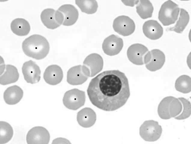
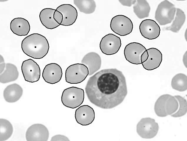
Figure 12 shows an example image with a set of reference locations that we selected manually and the optimal convex object found around each reference point. There are 14 reference locations and we used $N=30$ and $R=60$ to parametrize each object. Table 1 compares the running time of different optimization algorithms we implemented for this problem. Each line shows the time it took to solve all 14 problems contained in the example image using a particular search algorithm. The standard DP algorithm uses the dynamic programming solution outlined above. The CFDP method is based on the algorithm by ? (?) but modified for our representation of convex objects. Our hierarchical A* algorithm uses the abstraction hierarchy described here. For A* with pattern databases we used dynamic programming to compute a pattern database at a particular level of abstraction, and then used this database to provide heuristic values for A*. Note that for the problem described here the pattern database depends on the input. The running times listed include the time it took to compute the pattern database in each case.

We see that CFDP, HA*LD and A* with pattern databases are much more efficient than the standard dynamic programming algorithm that does not use abstractions. HA*LD is slightly faster then the other methods in this example. Note that while the running time varies from algorithm to algorithm the output of every method is the same as they all find globally optimum objects.

(a)

(b)

Figure 12: (a) Reference locations. (b) Optimal convex objects.

Standard DP	6718.6 seconds
CFDP	13.5 seconds
HA*LD	8.6 seconds
A* with pattern database in $\Sigma_{2}$	14.3 seconds
A* with pattern database in $\Sigma_{3}$	29.7 seconds

Table 1: Running time comparison for the example in Figure 12.

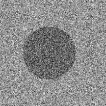
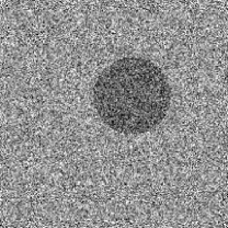
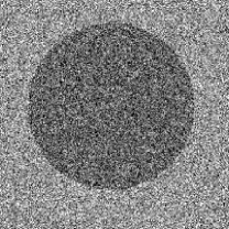
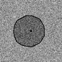
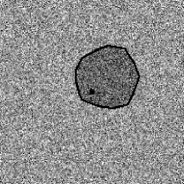
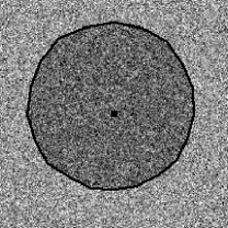
For a quantitative evaluation of the different search algorithms we created a large set of problems of varying difficulty and size as follows. For a given value of $R$ we generated square images of width and height $2*R+1$. Each image has a circle with radius less than $R$ near the center and the pixels in an image are corrupted by independent Gaussian noise. The difficulty of a problem is controlled by the standard deviation, $\sigma$, of the noise. Figure 13 shows some example images and optimal convex object found around their centers.

Figure 13: Random images with circles and the optimal convex object around the center of each one (with $N=20$ and $R=100$). The noise level in the images is $\sigma=50$.

The graph in Figure 14 shows the running time (in seconds) of the different search algorithms as a function of the noise level when the problem size is fixed at $R=100$. Each sample point indicates the average running time over 200 random inputs. The graph shows running times up to a point after which the circles can not be reliably detected. We compared HA*LD with CFDP and A* using pattern databases (PD2 and PD3). Here PD2 and PD3 refer to A* with a pattern database defined in $\Sigma_{2}$ and $\Sigma_{3}$ respectively. Since the pattern database needs to be recomputed for each input there is a trade-off in the amount of time spent computing the database and the accuracy of the heuristic it provides. We see that for easy problems it is better to use a smaller database (defined at a higher level of abstraction) while for harder problems it is worth spending time computing a bigger database. HA*LD outperforms the other methods in every situation captured here.

Figure 14: Running time of different search algorithms as a function of the noise level $\sigma$ in the input. Each sample point indicates the average running time taken over 200 random inputs. In each case $N=20$ and $R=100$. See text for discussion.

Figure 15: Running time of different search algorithms as a function of the problem size $R$. Each sample point indicates the average running time taken over 200 random inputs. In each case $N=20$ and $\sigma=100$. See text for discussion.

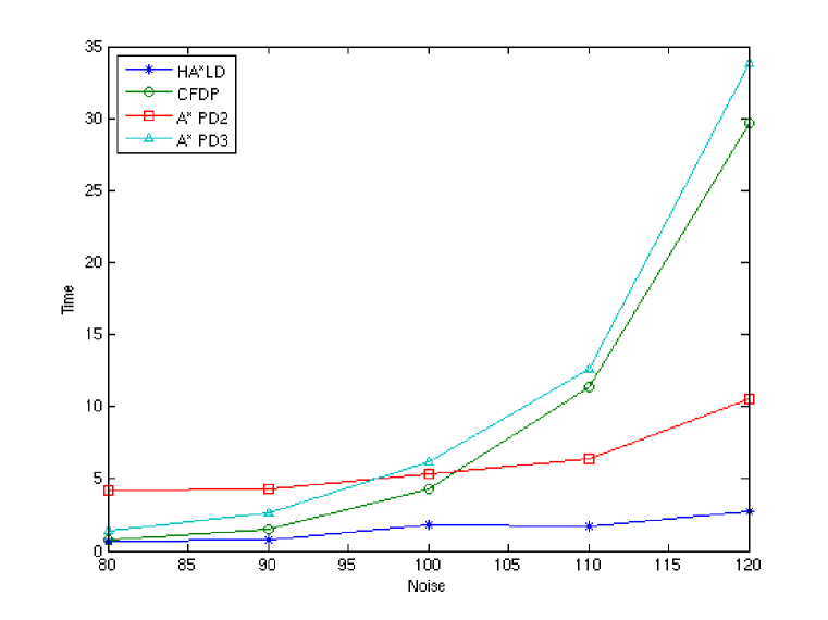
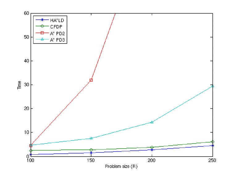
Figure 15 shows the running time of the different methods as a function of the problem size $R$, on problems with a fixed noise level of $\sigma=100$. As before each sample point indicates the average running time taken over 200 random inputs. We see that the running time of the pattern database approach grows quickly as the problem size increases. This is because computing the database at any fixed level of abstraction takes $O(NR^{5})$ time. On the other hand the running time of both CFDP and HA*LD grows much slower. While CFDP performed essentially as well as HA*LD in this experiment, the graph in Figure 14 shows that HA*LD performs better as the difficulty of the problem increases.

10 Finding Salient Curves in Images

A classical problem in computer vision involves finding salient curves in images. Intuitively the goal is to find long and smooth curves that go along paths with high image gradient. The standard way to pose the problem is to define a saliency score and search for curves optimizing that score. Most methods use a score defined by a simple combination of local terms. For example, the score usually depends on the curvature and the image gradient at each point of a curve. This type of score can often be optimized efficiently using dynamic programming or shortest paths algorithms (?, ?, ?, ?).

Here we consider a new compositional model for finding salient curves. An important aspect of this model is that it can capture global shape constraints. In particular, it looks for curves that are almost straight, something that can not be done using local constraints alone. Local constraints can enforce small curvature at each point of a curve, but this is not enough to prevent curves from turning and twisting around over long distances. The problem of finding the most salient curve in an image with the compositional model defined here can be solved using dynamic programming, but the approach is too slow for practical use. Shortest paths algorithms are not applicable because of the compositional nature of the model. Instead we can use A*LD with a heuristic function derived from an abstraction (a pattern database).

Figure 16: A curve with endpoints $(a,c)$ is formed by composing curves with endpoints $(a,b)$ and $(b,c)$. We assume that $t\geq\pi/2$. The cost of the composition is proportional to $\sin^{2}(t)$. This cost is scale invariant and encourages curves to be relatively straight.

Let $C_{1}$ be a curve with endpoints $a$ and $b$ and $C_{2}$ be a curve with endpoints $b$ and $c$. The two curves can be composed to form a curve $C$ from $a$ to $c$. We define the weight of the composition to be the sum of the weights of $C_{1}$ and $C_{2}$ plus a shape cost that depends on the geometric arrangement of points $(a,b,c)$. Figure 16 illustrates the idea and the shape costs we use. Note that when $C_{1}$ and $C_{2}$ are long, the arrangement of their endpoints reflect non-local geometric properties. In general we consider composing $C_{1}$ and $C_{2}$ if the angle formed by $\overline{ab}$ and $\overline{bc}$ is at least $\pi/2$ and the lengths of $C_{1}$ and $C_{2}$ are approximately equal. These constraints reduce the total number of compositions and play an important role in the abstract problem defined below.

Besides the compositional rule we say that if $a$ and $b$ are nearby locations, then there is a short curve with endpoints $a$ and $b$. This forms a base case for creating longer curves. We assume that these short curves are straight, and their weight depends only on the image data along the line segment from $a$ to $b$. We use a data term, $\text{\emph{seg}}(a,b)$, that is zero if the image gradient along pixels in $\overline{ab}$ is perpendicular to $\overline{ab}$, and higher otherwise.

Figure 10 gives a formal definition of the two rules in our model. The constants $k_{1}$ and $k_{2}$ specify the minimum and maximum length of the base case curves, while $L$ is a constant controlling the maximum depth of derivations. A derivation of $\text{\emph{curve}}(a,b,i)$ encodes a curve from $a$ to $b$. The value $i$ can be seen as an approximate measure of arclength. A derivation of $\text{\emph{curve}}(a,b,i)$ is a full binary tree of depth $i$ that encodes a curve with length between $2^{i}k_{1}$ and $2^{i}k_{2}$. We let $k_{2}=2k_{1}$ to allow for curves of any length.

(1) for pixels $a,b,c$ where the angle between $\overline{ab}$ and $\overline{bc}$ is at least $\pi/2$ and for $0\leq i\leq L$,

$\text{\emph{curve}}(a,b,i)=w_{1}$

$\text{\emph{curve}}(b,c,i)=w_{2}$

$\text{\emph{curve}}(a,c,i+1)=w_{1}+w_{2}+\text{\emph{shape}}(a,b,c)$

(2) for pixels $a,b$ with $k_{1}\leq||a-b||\leq k_{2}$,

$\text{\emph{curve}}(a,b,0)=\text{\emph{seg}}(a,b)$

Figure 17: Rules for finding “almost straight” curves between a pair of endpoints. Here $L$, $k_{1}$ and $k_{2}$ are constants, while $\text{\emph{shape}}(a,b,c)$ is a function measuring the cost of a composition.

The rules in Figure 10 do not define a good measure of saliency by themselves because they always prefer short curves over long ones. We can define the saliency of a curve in terms of its weight minus its arclength, so that salient curves will be light and long. Let $\lambda$ be a positive constant. We consider finding the lightest derivation of goal using,

$\text{\emph{curve}}(a,b,i)=w$

$\text{\emph{goal}}=w-\lambda 2^{i}$

For an $n\times n$ image there are $\Omega(n^{4})$ statements of the form $\text{\emph{curve}}(a,c,i)$. Moreover, if $a$ and $c$ are far apart there are $\Omega(n)$ choices for a “midpoint” $b$ defining the two curves that are composed in a lightest derivation of $\text{\emph{curve}}(a,c,i)$. This makes a dynamic programming solution to the lightest derivation problem impractical. We have tried using KLD but even for small images the algorithm runs out of memory after a few minutes. Below we describe an abstraction we have used to define a heuristic function for A*LD.

Consider a hierarchical set of partitions of an image into boxes. The $i$-th partition is defined by tiling the image into boxes of $2^{i}\times 2^{i}$ pixels. The partitions form a pyramid with boxes of different sizes at each level. Each box at level $i$ is the union of 4 boxes at the level below it, and the boxes at level 0 are the pixels themselves. Let $f_{i}(a)$ be the box containing $a$ in the $i$-th level of the pyramid. Now define

$$\text{\emph{abs}}(\text{\emph{curve}}(a,b,i))=\text{\emph{curve}}(f_{i}(a),f_{i}(b),i).$$

Figure 18 illustrates how this map selects a pyramid level for an abstract statement. Intuitively abs defines an adaptive coarsening criteria. If $a$ and $b$ are far from each other, a curve from $a$ to $b$ must be long, which in turn implies that we map $a$ and $b$ to boxes in a coarse partition of the image. This creates an abstract problem that has a small number of statements without losing too much information.

To define the abstract problem we also need to define a set of abstract rules. Recall that for every concrete rule $r$ we need a corresponding abstract rule $r^{\prime}$ where the weight of $r^{\prime}$ is at most the weight of $r$. There are a small number of rules with no antecedents in Figure 10. For each concrete rule $\rightarrow_{\text{\emph{seg}}(a,b)}\text{\emph{curve}}(a,b,0)$ we define a corresponding abstract rule, $\rightarrow_{\text{\emph{seg}}(a,b)}\text{\emph{abs}}(\text{\emph{curve}}(a,b,0))$. The compositional rules from Figure 10 lead to abstract rules for composing curves between boxes,

$$\text{\emph{curve}}(A,B,i),\text{\emph{curve}}(B,C,i)\rightarrow_{v}\text{\emph{curve}}(A^{\prime},C^{\prime},i+1),$$

where $A$, $B$ and $C$ are boxes at the $i$-th pyramid level while $A^{\prime}$ and $C^{\prime}$ are the boxes at level $i+1$ containing $A$ and $C$ respectively. The weight $v$ should be at most $\text{\emph{shape}}(a,b,c)$ where $a$, $b$ and $c$ are arbitrary pixels in $A$, $B$ and $C$ respectively. We compute a value for $v$ by bounding the orientations of the line segments $\overline{ab}$ and $\overline{bc}$ between boxes.

Figure 18: The abstraction maps each curve statement to a statement about curves between boxes. If $i>j$ then $\text{\emph{curve}}(a,b,i)$ gets coarsened more than $\text{\emph{curve}}(c,d,j)$. Since light curves are almost straight, $i>j$ usually implies that $||a-b||>||c-d||$.

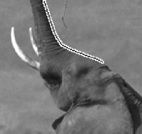
$146\times 137$ pixels. Running time: 50 seconds (38 + 12).

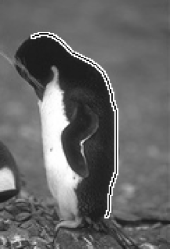
$122\times 179$ pixels. Running time: 65 seconds (43 + 22).

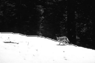
$226\times 150$ pixels. Running time: 73 seconds (61 + 12).

Figure 19: The most salient curve in different images. The running time is the sum of the time spent computing the pattern database and the time spent solving the concrete problem.

Figure 20: An example where the most salient curve goes over locations with essentially no local evidence for a the curve at those locations.

The abstract problem defined above is relatively small even in large images, so we can use the pattern database approach outlined in Section 5.1. For each input image we use KLD to compute lightest context weights for every abstract statement. We then use these weights as heuristic values for solving the concrete problem with A*LD. Figure 19 illustrates some of the results we obtained using this method. It seems like the abstract problem is able to capture that most short curves can not be extended to a salient curve. It took about one minute to find the most salient curve in each of these images. Figure 19 lists the dimensions of each image and the running time in each case.

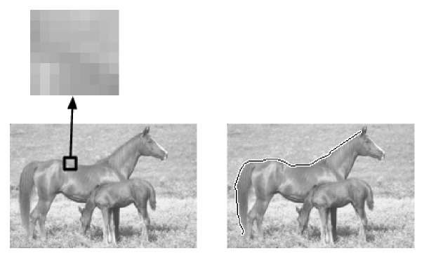
Note that our algorithm does not rely on an initial binary edge detection stage. Instead the base case rules allow for salient curves to go over any pixel, even if there is no local evidence for a boundary at a particular location. Figure 20 shows an example where this happens. In this case there is a small part of the horse back that blends with the background if we consider local properties alone.

The curve finding algorithm described in this section would be very difficult to formulate without A*LD and the general notion of heuristics derived from abstractions for lightest derivation problems. However, using the framework introduced in this paper it becomes relatively easy to specify the algorithm.

In the future we plan to “compose” the rules for computing salient curves with rules for computing more complex structures. The basic idea of using a pyramid of boxes for defining an abstract problem should be applicable to a variety of problems in computer vision.

11 Conclusion

Although we have presented some preliminary results in the last two sections, we view the main contribution of this paper as providing a general architecture for perceptual inference. Dijkstra’s shortest paths algorithm and A* search are both fundamental algorithms with many applications. Knuth noted the generalization of Dijkstra’s algorithm to more general problems defined by a set of recursive rules. In this paper we have given similar generalizations for A* search and heuristics derived from abstractions. We have also described a new method for solving lightest derivation problems using a hierarchy of abstractions. Finally, we have outlined an approach for using these generalizations in the construction of processing pipelines for perceptual inference.

Acknowledgments

This material is based upon work supported by the National Science Foundation under Grant No. 0535174 and 0534820.

References

- Basri and Alter Basri, R., and Alter, T. (1996). Extracting salient curves from images: An analysis of the saliency network. In IEEE Conference on Computer Vision and Pattern Recognition.
- Bonet and Geffner Bonet, B., and Geffner, H. (2005). An algorithm better than AO*. In Proceedings of the National Conference on Artificial Intelligence.
- Bulitko et al. Bulitko, V., Sturtevant, N., Lu, J., and Yau, T. (2006). State abstraction in real-time heuristic search. Technical Report, University of Alberta, Department of Computer Science.
- Charniak Charniak, E. (1996). Statistical Language Learning. MIT Press.
- Culberson and Schaeffer Culberson, J., and Schaeffer, J. (1998). Pattern databases. Computational Intelligence, 14(3), 318–334.
- Dijkstra Dijkstra, E. (1959). A note on two problems in connection with graphs. Numerical Mathematics, 1, 269–271.
- Edelkamp Edelkamp, S. (2002). Symbolic pattern databases in heuristic search panning. In International Conference on AI Planning and Scheduling.
- Felner Felner, A. (2005). Finding optimal solutions to the graph partitioning problem with heuristic search. Annals of Mathematics and Artificial Intelligence, 45(3-4), 293–322.
- Geman et al. Geman, S., Potter, D., and Chi, Z. (2002). Composition systems. Quarterly of Applied Mathematics, 707–736.
- Hansen and Zilberstein Hansen, E., and Zilberstein, S. (2001). LAO*: A heuristic search algorithm that finds solutions with loops. Artificial Intelligence, 129, 35–62.
- Hart et al. Hart, P., Nilsson, N., and Raphael, B. (1968). A formal basis for the heuristic determination of minimal cost paths. IEEE Transactions on Systems Science and Cybernetics, 4(2), 100–107.
- Holte et al. Holte, R., Grajkowski, J., and Tanner, B. (2005). Hierarchical heuristic search revisited. In Symposium on Abstraction, Reformulation and Approximation.
- Holte et al. Holte, R., Perez, M., Zimmer, R., and MacDonald, A. (1996). Hierarchical A*: Searching abstraction hierarchies efficiently. In Proceedings of the National Conference on Artificial Intelligence.
- Jimenez and Torras Jimenez, P., and Torras, C. (2000). An efficient algorithm for searching implicit AND/OR graphs with cycles. Artificial Intelligence, 124, 1–30.
- Jin and Geman Jin, Y., and Geman, S. (2006). Context and hierarchy in a probabilistic image model. In IEEE Conference on Computer Vision and Pattern Recognition.
- Klein and Manning Klein, D., and Manning, C. (2003). A* parsing: Fast exact viterbi parse selection. In Proceedings of the HLT-NAACL.
- Knuth Knuth, D. (1977). A generalization of Dijkstra’s algorithm. Information Processing Letters, 6(1), 1–5.
- Korf Korf, R. (1997). Finding optimal solutions to Rubik’s cube using pattern databases. In Proceedings of the National Conference on Artificial Intelligence.
- Korf and Felner Korf, R., and Felner, A. (2002). Disjoint pattern database heuristics. Artificial Intelligence, 134, 9–22.
- Korf et al. Korf, R., Zhang, W., Thayer, I., and Hohwald, H. (2005). Frontier search. Journal of the ACM, 52(5), 715–748.
- McAllester McAllester, D. (2002). On the complexity analysis of static analyses. Journal of the ACM, 49(4), 512–537.
- Montanari Montanari, U. (1971). On the optimal detection of curves in noisy pictures. Communications of the ACM, 14(5).
- Nilsson Nilsson, N. (1980). Principles of Artificial Intelligence. Morgan Kaufmann.
- Pearl Pearl, J. (1984). Heuristics: intelligent search strategies for computer problem solving. Addison-Wesley.
- Rabiner Rabiner, L. (1989). A tutorial on hidden Markov models and selected applications in speech recognition. Proceedings of the IEEE, 77(2), 257–286.
- Raphael Raphael, C. (2001). Coarse-to-fine dynamic programming. IEEE Transactions on Pattern Analysis and Machine Intelligence, 23(12), 1379–1390.
- Shashua and Ullman Shashua, A., and Ullman, S. (1988). Structural saliency: The detection of globally salient structures using a locally connected network. In IEEE International Conference on Computer Vision.
- Tu et al. Tu, Z., Chen, X., Yuille, A., and Zhu, S. (2005). Image parsing: Unifying segmentation, detection, and recognition. International Journal of Computer Vision, 63(2), 113–140.
- Williams and Jacobs Williams, L., and Jacobs, D. (1996). Local parallel computation of stochastic completion fields. In IEEE Conference on Computer Vision and Pattern Recognition.
- Zhang and Korf Zhang, W., and Korf, R. (1996). A study of complexity transitions on the asymmetric traveling salesman problem. Artificial Intelligence, 81, 1–2.