Closed-Loop Learning of Visual Control Policies

Abstract

In this paper we present a general, flexible framework for learning mappings from images to actions by interacting with the environment. The basic idea is to introduce a feature-based image classifier in front of a reinforcement learning algorithm. The classifier partitions the visual space according to the presence or absence of few highly informative local descriptors that are incrementally selected in a sequence of attempts to remove perceptual aliasing. We also address the problem of fighting overfitting in such a greedy algorithm. Finally, we show how high-level visual features can be generated when the power of local descriptors is insufficient for completely disambiguating the aliased states. This is done by building a hierarchy of composite features that consist of recursive spatial combinations of visual features. We demonstrate the efficacy of our algorithms by solving three visual navigation tasks and a visual version of the classical “Car on the Hill” control problem.

1 Introduction

Designing robotic controllers quickly becomes a challenging problem. Indeed, such controllers face a huge number of possible inputs that can be noisy, must select actions among a continuous set, and should be able to automatically adapt themselves to evolving or stochastic environmental conditions. Although a real-world robotic task can often be solved by directly connecting the perceptual space to the action space through a given computational mechanism, such mappings are usually hard to derive by hand, especially when the perceptual space contains images. Evidently, automatic methods for generating such mappings are highly desirable, because many robots are nowadays equipped with CCD sensors.

In this paper, we are interested in reactive systems that learn to couple visual perceptions and actions inside a dynamic world so as to act reasonably. This coupling is known as a visual (control) policy. This wide category of problems will be called vision-for-action tasks (or simply visual tasks). Despite about fifty years years of active research in artificial intelligence, robotic agents are still largely unable to solve many real-world visuomotor tasks that are easily performed by humans and even by animals. Such vision-for-action tasks notably include grasping, vision-guided navigation and manipulation of objects so as to achieve a goal. This article introduces a general framework that is suitable for building image-to-action mappings using a fully automatic and flexible learning protocol.

1.1 Vision-for-Action and Reinforcement Learning

Strong neuropsychological evidence suggests that human beings learn to extract useful information from visual data in an interactive fashion, without any external supervisor (?). By evaluating the consequence of our actions on the environment, we learn to pay attention to visual cues that are behaviorally important for solving the task. This way, as we interact with the outside world, we gain more and more expertise on our tasks (?). Obviously, this process is task driven, since different tasks do not necessarily need to make the same distinctions (?).

A breakthrough in modern artificial intelligence would be to design an artificial system that would acquire object or scene recognition skills based only on its experience with the surrounding environment. To state it in more general terms, an important research direction would be to design a robotic agent that could autonomously acquire visual skills from its interactions with an uncommitted environment in order to achieve some set of goals. Learning new visual skills in a dynamic, task-driven fashion so as to complete an a priori unknown visual task is known as the purposive vision paradigm (?).

One plausible framework to learn image-to-action mappings according to purposive vision is Reinforcement Learning (RL) (?, ?, ?). Reinforcement learning is a biologically-inspired computational framework that can generate nearly optimal control policies in an automatic way, by interacting with the environment. RL is founded on the analysis of a so-called reinforcement signal. Whenever the agent takes a decision, it receives as feedback a real number that evaluates the relevance of this decision. From a biological perspective, when this signal becomes positive, the agent experiences pleasure, and we can talk about a reward. Conversely, a negative reinforcement implies a sensation of pain, which corresponds to a punishment. The reinforcement signal can be arbitrarily delayed from the actions which are responsible for it. Now, RL algorithms are able to map every possible perception to an action that maximizes the reinforcement signal over time. In this framework, the agent is never told what the optimal action is when facing a given percept, nor whether one of its decisions was optimal. Rather, the agent has to discover by itself what the most promising actions are by constituting a representative database of interactions, and by understanding the influence of its decisions on future reinforcements. Schematically, RL lies between supervised learning (where an external teacher gives the correct action to the agent) and unsupervised learning (in which no clue about the goodness of the action is given).

RL has had successful applications, for example turning a computer into an excellent Backgammon player (?), solving the Acrobot control problem (?), making a quadruped robot learn progressively to walk without any human intervention (?, ?, ?), riding a bicycle (?, ?) or controlling a helicopter (?, ?). The major advantages of the RL protocol are that it is fully automatic, and that it imposes very weak constraints on the environment.

Unfortunately, standard RL algorithms are highly sensitive to the number of distinct percepts as well as to the noise that results from the sensing process. This general problem is often referred to as the Bellman curse of dimensionality (?). Thus, the high dimensionality and the noise that is inherent to images forbid the use of basic RL algorithms for direct closed-loop learning of image-to-action mappings according to purposive vision.

1.2 Achieving Purposive Vision through Reinforcement Learning

There exists a variety of work in RL on specific robotic problems involving a perceptual space that contains images. For instance, Schaal (?) uses visual feedback to solve a pole-balancing task. RL has been used to control a vision-guided underwater robotic vehicle (?). More recently, Kwok and Fox (?) have demonstrated the applicability of RL to learning sensing strategies using Aibo robots. Reinforcement learning can also be used to learn strategies for view selection (?) and sequential attention models (?). Let us also mention the use of reinforcement learning in other vision-guided tasks such as ball kicking (?), ball acquisition (?), visual servoing (?), robot docking (?, ?) and obstacle avoidance (?). Interestingly, RL is also used as a way of tuning the high-level parameters of image-processing applications. For example, Peng and Bhanu (?) introduce RL algorithms for image segmentation, whereas Yin (?) proposes algorithms for multilevel image thresholding, and uses entropy as a reinforcement signal.

All of these applications preprocess the images to extract some high-level information about the observed scene that is directly relevant to the task to be solved and that feeds the RL algorithm. This requires prior assumptions about the images perceived by the sensors of the agent, and about the physical structure of the task itself. The preprocessing step is task specific and is coded by hand. This contrasts with our objectives, which consist in introducing algorithms able to learn how to directly connect the visual space to the action space, without using manually written code and without relying on prior knowledge about the task to be solved. Our aim is to develop general algorithms that are applicable to any visual task that can be formulated in the RL framework.

A noticeable exception is the work by Iida et al. (?) who apply RL to seek and reach targets, and to push boxes (?) with real robots. In this work, raw visual signals directly feed a neural network that is trained by an actor-critic architecture. In these examples, the visual signal is downscaled and averaged into a monochrome (i.e. two-color) image of $64\times 24=1536$ pixels. The output of four infrared sensors are also added to this perceptual input. While this approach is effective for the specific tasks, this process can only be used in a highly controlled environment. Real-world images are much richer and could not undergo such a strong reduction in size.

1.3 Local-Appearance Paradigm

In this paper, we propose algorithms that rely on the extraction of visual features as a way to achieve more compact state spaces that can be used as an input to traditional RL algorithms. Indeed, buried in the noise and in the confusion of visual cues, images contain hints of regularity. Such regularities are captured by the important notion of visual features. Loosely speaking, a visual feature is a representation of some aspect of local appearance, e.g. a corner formed by two intensity edges, a spatially localized texture signature, or a color. Therefore, to analyze images, it is often sufficient for a computer program to extract only useful information from the visual signal, by focusing its attention on robust and highly informative patterns in the percepts. The program should thereafter seek the characteristic appearance of the observed scenes or objects.

This is actually the basic postulate behind local-appearance methods that have had much success in computer vision applications such as image matching, image retrieval and object recognition (?, ?). They rely on the detection of discontinuities in the visual signal thanks to interest point detectors (?). Similarities in images are thereafter identified using a local description of the neighborhood around the interest points (?): If two images share a sufficient number of matching local descriptors, they are considered to belong to the same visual class.

Local-appearance techniques are at the same time powerful and flexible, as they are robust to partial occlusions, and do not require segmentation or 3D models of the scenes. It seems therefore promising to introduce, in front of the RL algorithm, a feature-based image classifier that partitions the visual space into a finite set of distinct visual classes according to the local-appearance paradigm, by focusing the attention of the agent on highly distinctive local descriptors located at interest points of the visual stimuli. The symbol corresponding to the detected visual class could then be given as the input of a classical, embedded RL algorithm, as shown in Figure 1.

This preprocessing step is intended to reduce the size of the input domain, thus enhancing the rate of convergence, the generalization capabilities as well as the robustness of RL to noise in visual domains. Importantly, the same family of visual features can be applied to a wide variety of visual tasks, thus the preprocessing step is essentially general and task-independent. The central difficulty is the dynamic selection of the discriminative visual features. This selection process should group images that share similar, task-specific properties together in the same visual class.

Figure 1: The structure of Reinforcement Learning of Visual Classes.

1.4 Contributions

The key technical contribution of this paper consists in the introduction of reinforcement learning algorithms that can be used when the perceptual space contains images. The developed algorithms do not rely on a task-specific pre-treatment. As a consequence, they can be used in any vision-for-action task that can be formalized as a Markov Decision Problem. We now review the three major contributions that are discussed in this paper.

1.4.1 Adaptive Discretization of a Visual Space

Our first contribution is to propose a new algorithm called Reinforcement Learning of Visual Classes (RLVC) that combines the aforementioned ideas. RLVC is an iterative algorithm that is suitable for learning direct image-to-action mappings by taking advantage of the local-appearance paradigm. It consists of two simultaneous, interleaved learning processes: Reinforcement learning of a mapping from visual classes to actions, and incremental building of a feature-based image classifier.

Initially, the image classifier contains one single visual class, so that all images are mapped to this class. Of course, this introduces a kind of perceptual aliasing (or hidden state) (?): The optimal decisions cannot always be made, since percepts requiring different reactions are associated with the same class. The agent then isolates the aliased classes. Since there is no external supervisor, the agent can only rely on a statistical analysis of the earned reinforcements. For each detected aliased class, the agent dynamically selects a new visual feature that is distinctive, i.e. that best disambiguates the aliased percepts. The extracted local descriptor is used to refine the classifier. This way, at each stage of the algorithm, the number of visual classes in the classifier grows. New visual features are learned until perceptual aliasing vanishes. The resulting image classifier is finally used to control the system.

Our approach is primarily motivated by strong positive results of McCallum’s U-Tree algorithm (?). In essence, RLVC is an adaptation of U-Tree to visual spaces, though the internals of the algorithms are different. The originality of RLVC lies in its exploitation of successful local-appearance features. RLVC selects a subset of such highly relevant features in a fully closed-loop, purposive learning process. We show that this algorithm is of practical interest, as it can be successfully applied to several simulated visual navigation tasks.

1.4.2 Compacting Visual Policies

Because of its greedy nature, RLVC is prone to overfitting. Splitting one visual class can potentially improve the control policy for all the visual classes. Therefore, the splitting strategy can get stuck in local minima: Once a split is made that subsequently proves useless, it cannot be undone in the original description of RLVC. Our second contribution is to provide RLVC with the possibility of aggregating visual classes that share similar properties. Doing so has at least three potential benefits:

1. Useless features are discarded, which enhances generalization capabilities;

2. RLVC can reset the search for good features; and

3. the number of samples that the embedded RL algorithm has at its disposal for each visual class is increased, which results in better visual control policies.

Experiments indeed show an improvement in the generalization abilities, as well as a reduction of the number of visual classes and selected features.

1.4.3 Spatial Combinations of Visual Features

Finally, the efficacy of RLVC clearly depends on the discriminative power of the visual features. If their power is insufficient, the algorithm will not be able to completely remove the aliasing, which will produce sub-optimal control policies. Practical experiments on simulated visual navigation tasks exhibit this deficiency, as soon as the number of detected visual features is reduced or as features are made more similar by using a less sensitive metric. Now, most objects encountered in the world are composed of a number of distinct constituent parts (e.g. a face contains a nose and two eyes, a phone possesses a keypad). These parts are themselves recursively composed of other sub-parts (e.g. an eye contains an iris and eyelashes, a keypad is composed of buttons). Such a hierarchical physical structure certainly imposes strong constraints on the spatial disposition of the visual features.

Our third contribution is to show how highly informative spatial combinations of visual features can be iteratively constructed in the framework of RLVC. This result is promising for it permits the construction of features at increasingly higher levels of discriminative power, enabling us to tackle visual tasks that are unsolvable using individual point features alone. To the best of our knowledge, this extension to RLVC appears to be the very first attempt to build visual feature hierarchies in a closed-loop, interactive and purposive learning process.

2 An Overview of Reinforcement Learning

Our framework relies on the theory of RL, which is introduced in this section. In RL, the environment is traditionally modeled as a Markov Decision Process (MDP). An MDP is a tuple $\langle S,A,{\cal T},{\cal R}\rangle$, where $S$ is a finite set of states, $A$ is a finite set of actions, $\cal T$ is a probabilistic transition function from $S\times A$ to $S$, and $\cal R$ is a reinforcement function from $S\times A$ to $\mathbb{R}$. An MDP obeys the following discrete-time dynamics: If at time $t$, the agent takes the action $a_{t}$ while the environment lies in a state $s_{t}$, the agent perceives a numerical reinforcement $r_{t+1}={\cal R}(s_{t},a_{t})$, then reaches some state $s_{t+1}$ with probability ${\cal T}(s_{t},a_{t},s_{t+1})$. Thus, from the point of view of the agent, an interaction with the environment is defined as a quadruple $\langle s_{t},a_{t},r_{t+1},s_{t+1}\rangle$. Note that the definition of Markov decision processes assumes the full observability of the state space, which means that the agent is able to distinguish between the states of the environment using only its sensors. This allows us to talk indifferently about states and percepts. In visual tasks, $S$ is a set of images.

A percept-to-action mapping is a fixed probabilistic function $\pi:S\mapsto A$ from states to actions. A percept-to-action mapping tells the agent the probability with which it should choose an action when faced with some percept. In RL terminology, such a mapping is called a stationary Markovian control policy. For an infinite sequence of interactions starting in a state $s_{t}$, the discounted return is

$$R_{t}=\sum_{i=0}^{\infty}\gamma^{i}r_{t+i+1},$$ (1)

where $\gamma\in[0,1[$ is the discount factor that gives the current value of the future reinforcements. The Markov decision problem for a given MDP is to find an optimal percept-to-action mapping that maximizes the expected discounted return, whatever the starting state is. It is possible to prove that this problem is well-defined, in that such an optimal percept-to-action mapping always exists (?).

Markov decision problems can be solved using Dynamic Programming (DP) algorithms (?, ?). Let $\pi$ be a percept-to-action mapping. Let us call the state-action value function $Q^{\pi}(s,a)$ of $\pi$, the function giving for each state $s\in S$ and each action $a\in A$ the expected discounted return obtained by starting from state $s$, taking action $a$, and thereafter following the mapping $\pi$:

$$Q^{\pi}(s,a)={\rm E}^{\pi}\left\{R_{t}\mid s_{t}=s,a_{t}=a\right\},$$ (2)

where ${\rm E}^{\pi}$ denotes the expected value if the agent follows the mapping $\pi$. Let us also define the $H$ transform from $Q$ functions to $Q$ functions as

$$(HQ)(s,a)={\cal R}(s,a)+\gamma\sum_{s^{\prime}\in S}{\cal T}(s,a,s^{\prime})\max_{a^{\prime}\in A}Q(s^{\prime},a^{\prime}),$$ (3)

for all $s\in S$ and $a\in A$. Note that the $H$ transform is equally referred to as the Bellman backup operator for state-action value functions. All the optimal mappings for a given MDP share the same $Q$ function, denoted $Q^{*}$ and called the optimal state-action value function, that always exists and that satisfies Bellman’s so-called optimality equation (?)

$$HQ^{*}=Q^{*}.$$ (4)

Once the optimal state-action value function $Q^{*}$ is known, an optimal deterministic percept-to-action mapping $\pi^{*}$ is easily derived by choosing

$$\pi^{*}(s)=\mathop{\rm argmax}_{a\in A}Q^{*}(s,a),$$ (5)

for each $s\in S$. Another very useful concept from the DP theory is that of optimal value function $V^{*}$. For each state $s\in S$, $V^{*}(s)$ corresponds to the expected discounted return when the agent always chooses the optimal action in each encountered state, i.e.

$$V^{*}(s)=\max_{a\in A}Q^{*}(s,a).$$ (6)

Dynamic Programming includes the well-known Value Iteration (?), Policy Iteration (?) and Modified Policy Iteration (?) algorithms. Value Iteration learns the optimal state-action value function $Q^{*}$, whereas Policy Iteration and Modified Policy Iteration directly learn an optimal percept-to-action mapping.

RL is a set of algorithmic methods for solving Markov decision problems when the underlying MDP is not known (?, ?, ?). Precisely, RL algorithms do not assume the knowledge of $\cal T$ and $\cal R$. The input of RL algorithms is basically a sequence of interactions $\langle s_{t},a_{t},r_{t+1},s_{t+1}\rangle$ of the agent with its environment. RL techniques are often divided in two categories:

1. Model-based methods that first build an estimate of the underlying MDP (e.g. by computing the relative frequencies that appear in the sequence of interactions), and then use classical DP algorithms such as Value or Policy Iteration;

2. Model-free methods such as SARSA (?), $TD(\lambda)$ (?, ?), and the popular $Q$-learning (?), that do not compute such an estimate.

3 Reinforcement Learning of Visual Classes

As discussed in the Introduction, we propose to insert an image classifier before the RL algorithm. This classifier maps the visual stimuli to a set of visual classes according to the local-appearance paradigm, by focusing the attention of the agent on highly distinctive local descriptors detected at the interest points of the images.

3.1 Incremental Discretization of the Visual Space

Formally, let us call $D$, the infinite set of local descriptors that can be spanned through the chosen local description method. The elements of $D$ will be equivalently referred to as visual features. Usually, $D$ corresponds to $\mathbb{R}^{n}$ for some $n\geq 1$. We assume the existence of a visual feature detector, that is a Boolean function ${\cal D}:S\times D\mapsto{\cal B}$ testing whether a given image exhibits a given local descriptor at one of its interest points (?). Any suitable metric can be used to test the similarity of two visual features, e.g. Mahalanobis or Euclidean distance.

The image classifier is iteratively refined. Because of this incremental process, a natural way to implement the image classifiers is to use binary decision trees. Each of their internal nodes is labeled by the visual feature, the presence of which is to be tested in that node. The leaves of the trees define a set of visual classes, which is hopefully much smaller than the original visual space, and upon which it is possible to apply directly any usual RL algorithm. To classify an image, the system starts at the root node, then progresses down the tree according to the result of the feature detector $\cal D$ for each visual feature found during the descent, until reaching a leaf.

To summarize, RLVC builds a sequence ${\cal C}_{0},{\cal C}_{1},{\cal C}_{2},\ldots$ of growing decision trees, in a sequence of attempts to remove perceptual aliasing. The initial classifier ${\cal C}_{0}$ maps all of its input images in a single visual class $V_{0,1}$. At any stage $k$, the classifier ${\cal C}_{k}$ partitions the visual perceptual space $S$ into a finite number $m_{k}$ of visual classes $\{V_{k,1},\ldots,V_{k,m_{k}}\}$.

3.2 Learning Architecture

The resulting learning architecture has been called Reinforcement Learning of Visual Classes (RLVC) (?). The basic idea behind our algorithms, namely the iterative learning of a decision tree, is primarily motivated by adaptive-resolution techniques that have been previously introduced in reinforcement learning, and notably by McCallum’s U-Tree algorithm (?). In this section, this idea is showed to be extremely fruitful when suitably adapted to visual spaces. The links between RLVC and adaptive-resolution techniques will be more thoroughly discussed in Section 3.6.

Figure 2: The different components of the RLVC algorithm.

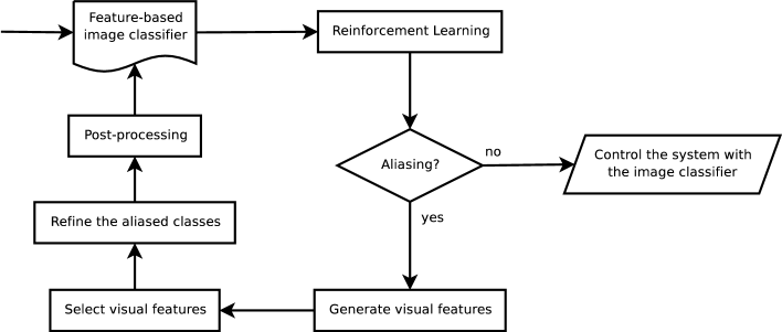
The components of RLVC are depicted in Figure 2. An in-depth discussion of each of those components will be given in the next sections. For the time being, we review each of them:

RL algorithm:

For each classifier in the sequence, an arbitrary, standard RL algorithm is applied. This provides information such as the optimal state-action function, the optimal value function or the optimal policy that are induced by the current classifier ${\cal C}_{k}$. For the purpose of these computations, either new interactions can be acquired, or a database of previously collected interactions can be exploited. This component is covered in Sections 3.3.1 and 3.3.2.

Aliasing detector:

Until the agent has learned the visual classes required to complete its task, from the viewpoint of the embedded RL algorithm, the input space is only partially observable. The aliasing detector extracts the classes in which perceptual aliasing occurs, through an analysis of the Bellman residuals. Indeed, as explained in Section 3.3.3, there exist tight relations between perceptual aliasing and Bellman residuals. If no aliased class is detected, RLVC stops.

Feature generator:

After having applied the RL algorithm, a database of interactions $\langle s_{t},a_{t},r_{t+1},s_{t+1}\rangle$ is available. The feature generator component produces a set $F$ of candidate visual features for each aliased class $V_{k,i}$. The features that are used to refine a classifier will be chosen among this set of candidates. This step is further exposed in Sections 3.4 and 5.

Feature selector:

Once the set of candidate features $F$ is built for the aliased visual class $V_{k,i}$, this component selects the visual feature $f^{*}\in F$ that best reduces the perceptual aliasing. If no candidate feature is discriminant, the component returns the conventional bottom symbol $\perp$. The feature selector of RLVC is described in Section 3.4.

Classifier refinement:

The leaves that correspond to the aliased classes in the feature-based image classifier are replaced by an internal node testing the presence or absence of the selected visual features.

Post-processing:

This optional component is invoked after every refinement, and corresponds to techniques for fighting overfitting. Details are given in Section 4.

Algorithm 1 — General structure of RLVC

1:  $k\leftarrow 0$

2:  $m_{k}\leftarrow 1$

3:  ${\cal C}_{k}\leftarrow$ binary decision tree with one leaf

4:  repeat

5:     Collect $N$ interactions $\langle s_{t},a_{t},r_{t+1},s_{t+1}\rangle$

6:     Apply an arbitrary RL algorithm on the sequence that is mapped through ${\cal C}_{k}$

7:     ${\cal C}_{k+1}\leftarrow{\cal C}_{k}$

8:     for all $i\in\{1,\ldots,m_{k}\}$ do

9:        if $\mbox{\tt aliased}(V_{k,i})$ then

10:           $F\leftarrow\mbox{\tt generator}\left(\left\{s_{t}\mid{\cal C}_{k}(s_{t})=V_{k,i}\right\}\right)$

11:           $f^{*}\leftarrow\mbox{\tt selector}\left(V_{k,i},F\right)$

12:           if $f^{*}\not=\ \perp$ then

13:              In ${\cal C}_{k+1}$, refine $V_{k,i}$ by testing $f^{*}$

14:              $m_{k+1}\leftarrow m_{k+1}+1$

15:           end if

16:        end if

17:     end for

18:     $k\leftarrow k+1$

19:     $\mbox{\tt post-process}({\cal C}_{k})$

20:  until ${\cal C}_{k}={\cal C}_{k-1}$

The general outline of RLVC is described in Algorithm 1. Note that in all the experiments that are contained in this paper, model-based RL algorithms were applied to static databases of interactions at the fifth step of Algorithm 1. These databases were collected using a fully randomized exploration policy. This choice was only guided by the ease of implementation and presentation; any other way of collecting experience could be used as well, for example by re-sampling a new database of interactions at each iteration of RLVC. The crucial point here is that RLVC generates a representation for visual control policies only from a set of collected visuomotor experience, which makes RLVC interactive. The following sections describe the remaining algorithms, namely aliased, generator, selector and post-process.

3.3 Detection of the Aliased Visual Classes

We now discuss how aliasing can be detected in a classifier ${\cal C}_{k}$.

3.3.1 Projection of an MDP through an Image Classifier

Formally, any image classifier ${\cal C}_{k}$ converts a sequence of $N$ interactions

$$\langle s_{t},a_{t},r_{t+1},s_{t+1}\rangle,$$

to a mapped sequence of $N$ quadruples

$$\langle{\cal C}_{k}(s_{t}),a_{t},r_{t+1},{\cal C}_{k}(s_{t+1})\rangle,$$

upon which the embedded RL algorithm is applied. Let us define the mapped MDP ${\cal M}_{k}$ as the MDP

$$\langle S_{k},A,{\cal T}_{k},{\cal R}_{k}\rangle,$$

that is obtained from the mapped sequence, where $S_{k}$ is the set of visual classes that are known to ${\cal C}_{k}$, and where ${\cal T}_{k}$ and ${\cal R}_{k}$ have been computed using the relative frequencies in the mapped sequence, as follows.

Consider two visual classes $V,V^{\prime}\in\{V_{k,1},\ldots,V_{k,m_{k}}\}$ and one action $a\in A$. We define the following functions:

• $\delta_{t}(V,a)$ equals $1$ if ${\cal C}_{k}(s_{t})=V$ and $a_{t}=a$, and $0$ otherwise;

• $\delta_{t}\left(V,a,V^{\prime}\right)$ equals $1$ if ${\cal C}_{k}(s_{t})=V$, ${\cal C}_{k}(s_{t+1})=V^{\prime}$ and $a_{t}=a$, and $0$ otherwise;

• $\eta(V,a)$ is the number of $t$’s such that $\delta_{t}(V,a)=1$.

Using this notation, we can write:

• $S_{k}=\left\{V_{k,1},\ldots,V_{k,m_{k}}\right\}$;

• ${\cal T}_{k}\left(V,a,V^{\prime}\right)=\sum_{t=1}^{N}\delta_{t}\left(V,a,V^{\prime}\right)/\eta(V,a)$;

• ${\cal R}_{k}(V,a)=\sum_{t=1}^{N}r_{t}\delta_{t}(V,a)/\eta(V,a)$.

3.3.2 Optimal $Q$ Function for a Mapped MDP

Each mapped MDP ${\cal M}_{k}$ induces an optimal $Q$ function on the domain $S_{k}\times A$ that will be denoted $Q^{\prime*}_{k}$. Computing $Q^{\prime*}_{k}$ can be difficult: In general, there may exist no MDP defined on the state space $S_{k}$ and on the action space $A$ that can generate a given mapped sequence, since the latter is not necessarily Markovian anymore. Thus, if some RL algorithm is run on the mapped sequence, it might not converge toward $Q^{\prime*}_{k}$, or not even converge at all. However, when applied on a mapped sequence, any model-based RL method (cf. Section 2) can be used to compute $Q^{\prime*}_{k}$ if ${\cal M}_{k}$ is used as the underlying model. Under some conditions, $Q$-learning also converges to the optimal $Q$ function of the mapped MDP (?).

In turn, the function $Q^{\prime*}_{k}$ induces another $Q$ function on the initial domain $S\times A$ through the relation:

$$Q^{*}_{k}(s,a)=Q^{\prime*}_{k}\left({\cal C}_{k}(s),a\right),$$ (7)

In the absence of aliasing, the agent would perform optimally, and $Q^{*}_{k}$ would correspond to $Q^{*}$, according to Bellman theorem that states the uniqueness of the optimal $Q$ function (cf. Section 2). By Equation 4, the function

$$B_{k}(s,a)=(HQ^{*}_{k})(s,a)-Q^{*}_{k}(s,a)$$ (8)

is therefore a measure of the aliasing induced by the image classifier ${\cal C}_{k}$. In RL terminology, $B_{k}$ is Bellman residual of the function $Q^{*}_{k}$ (?). The basic idea behind RLVC is to refine the states that have a non-zero Bellman residual.

3.3.3 Measuring Aliasing

Consider a time stamp $t$ in a database of interactions $\langle s_{t},a_{t},r_{t+1},s_{t+1}\rangle$. According to Equation 8, the Bellman residual that corresponds to the state-action pair $(s_{t},a_{t})$ equals

$$B_{k}(s_{t},a_{t})={\cal R}(s_{t},a_{t})+\gamma\sum_{s^{\prime}\in S}{\cal T}(s_{t},a_{t},s^{\prime})\max_{a^{\prime}\in A}Q^{*}_{k}(s^{\prime},a^{\prime})-Q^{*}_{k}(s_{t},a_{t}).$$ (9)

Unfortunately, the RL agent does not have access to the transition probabilities $\cal T$ and to the reinforcement function $\cal R$ of the MDP modeling the environment. Therefore, Equation 9 cannot be directly evaluated. A similar problem arises in the $Q$-learning (?) and the Fitted $Q$ Iteration (?) algorithms. These algorithms solve this problem by considering the stochastic version of the time difference that is described by Equation 9: The value

$$\sum_{s^{\prime}\in S}{\cal T}(s_{t},a_{t},s^{\prime})\max_{a^{\prime}\in A}Q^{*}_{k}(s^{\prime},a^{\prime})$$ (10)

can indeed be estimated as

$$\max_{a^{\prime}\in A}Q^{*}_{k}(s^{\prime},a^{\prime}),$$ (11)

if the successor $s^{\prime}$ is chosen with probability ${\cal T}(s_{t},a_{t},s^{\prime})$. But following the transitions of the environment ensures making a transition from $s_{t}$ to $s_{t+1}$ with probability ${\cal T}(s_{t},a_{t},s_{t+1})$. Thus

$$\Delta_{t} = r_{t+1}+\gamma\max_{a^{\prime}\in A}Q^{*}_{k}(s_{t+1},a^{\prime})-Q^{*}_{k}(s_{t},a_{t})$$ (12)

$$= r_{t+1}+\gamma\max_{a^{\prime}\in A}Q^{\prime*}_{k}\left({\cal C}_{k}\left(s_{t+1}\right),a^{\prime}\right)-Q^{\prime*}_{k}({\cal C}_{k}(s_{t}),a)$$ (13)

is an unbiased estimate of the Bellman residual for the state-action pair $(s_{t},a_{t})$ (?). Very importantly, if the system is deterministic and in the absence of perceptual aliasing, these estimates are equal to zero. Therefore, a nonzero $\Delta_{t}$ potentially indicates the presence of perceptual aliasing in the visual class $V_{t}={\cal C}_{k}(s_{t})$ with respect to action $a_{t}$. Our criterion for detecting the aliased classes consists in computing the $Q^{\prime*}_{k}$ function, then in sweeping again all the interactions $\langle s_{t},a_{t},r_{t+1},s_{t+1}\rangle$ to identify nonzero $\Delta_{t}$. In practice, we assert the presence of aliasing if the variance of the $\Delta_{t}$ exceeds a given threshold $\tau$. This is summarized in Algorithm 2, where $\sigma^{2}(\cdot)$ denotes the variance of a set of samples.

Algorithm 2 — Aliasing Criterion

1:  $\mbox{\tt aliased}(V_{k,i})$ :–

2:     for all $a\in A$ do

3:        $\Delta\leftarrow\{\Delta_{t}\mid{\cal C}_{k}(s_{t})=V_{k,i}\wedge a_{t}=a\}$

4:        if $\sigma^{2}(\Delta)>\tau$ then

5:           return true

6:        end if

7:     end for

8:     return false

3.4 Generation and Selection of Distinctive Visual Features

Once aliasing has been detected in some visual class $V_{k,i}\in S_{k}$ with respect to an action $a$, we need to select a local descriptor that best explains the variations in the set of $\Delta_{t}$ values corresponding to $V_{k,i}$ and $a$. This local descriptor is to be chosen among a set of candidate visual features $F$.

3.4.1 Extraction of Candidate Features

Informally, the canonical way of building $F$ for a visual class $V_{k,i}$ consists in:

1. identifying all collected visual percepts $s_{t}$ such that ${\cal C}_{k}(s_{t})=V_{k,i}$,

2. locating all the interest points in all the selected images $s_{t}$, then

3. adding to $F$ the local descriptor of all those interest points.

The corresponding feature generator is detailed in Algorithm 3. In the latter algorithm, $\mbox{\tt descriptor}(s,x,y)$ returns the local description of the point at location $(x,y)$ in the image $s$, and $\mbox{\tt symbol}({\bf d})$ returns the symbol that corresponds to the local descriptor ${\bf d}\in F$ according to the used metric. However, more complex strategies for generating the visual features can be used. Such a strategy that builds spatial combinations of individual point features will be presented in Section 5.

Algorithm 3 — Canonical feature generator

1:  $\mbox{\tt generator}(\{s_{1},\ldots,s_{n}\})$ :–

2:     $F\leftarrow\{\}$

3:     for all $i\in\{1,\ldots,n\}$ do

4:        for all $(x,y)$ such that $(x,y)$ is an interest point of $s_{i}$ do

5:           $F\leftarrow F\cup\{\mbox{\tt symbol}(\mbox{\tt descriptor}(s_{i},x,y))\}$

6:        end for

7:     end for

8:     return $F$

3.4.2 Selection of Candidate Features

The problem of choosing the candidate feature that most reduces the variations in a set of real-valued Bellman residuals is a regression problem, for which we suggest an adaptation of a popular splitting rule used in the CART algorithm for building regression trees (?).

In CART, variance is used as an impurity indicator: The split that is selected to refine a particular node is the one that leads to the greatest reduction in the sum of the squared differences between the response values for the learning samples corresponding to the node and their mean. More formally, let $S=\{\langle{\bf x}_{i},y_{i}\rangle\}$ be a set of learning samples, where ${\bf x}_{i}\in\mathbb{R}^{n}$ are input vectors of real numbers, and where $y_{i}\in\mathbb{R}$ are real-valued outputs. CART selects the following candidate feature:

$$f^{*}=\mathop{\rm argmin}_{v\in F}\left(p^{v}_{\oplus}\cdot\sigma^{2}\left(S^{v}_{\oplus}\right)+p^{v}_{\ominus}\cdot\sigma^{2}\left(S^{v}_{\ominus}\right)\right),$$ (14)

where $p^{v}_{\oplus}$ (resp. $p^{v}_{\ominus}$) is the proportion of samples that exhibit (resp. do not exhibit) the feature $v$, and where $S^{v}_{\oplus}$ (resp. $S^{v}_{\ominus}$) is the set of samples that exhibit (resp. do not exhibit) the feature $v$. This idea can be directly transferred in our framework, if the set of ${\bf x}_{i}$ corresponds to the set of interactions $\langle s_{t},a_{t},r_{t+1},s_{t+1}\rangle$, and if the set of $y_{i}$ corresponds to the set of $\Delta_{t}$. This is written explicitly in Algorithm 4.

Algorithm 4 — Feature Selection

1:  $\mbox{\tt selector}(V_{k,i},F)$ :–

2:     $f^{*}\leftarrow\ \perp$        {Best feature found so far}

3:     $r^{*}\leftarrow+\infty$     {Variance reduction induced by $f^{*}$}

4:     for all $a\in A$ do

5:        $T\leftarrow\{t\mid{\cal C}_{k}(s_{t})=V_{k,i}\mbox{~{}and~{}}a_{t}=a\}$

6:        for all visual feature $f\in F$ do

7:           $S_{\oplus}\leftarrow\{\Delta_{t}\mid t\in T\mbox{~{}and~{}}s_{t}\mbox{~{}exhibits~{}}f\}$

8:           $S_{\ominus}\leftarrow\{\Delta_{t}\mid t\in T\mbox{~{}and~{}}s_{t}\mbox{~{}does not exhibit~{}}f\}$

9:           $s_{\oplus}\leftarrow|S_{\oplus}|/|T|$

10:           $s_{\ominus}\leftarrow|S_{\ominus}|/|T|$

11:           $r\leftarrow s_{\oplus}\cdot\sigma^{2}\left(S_{\oplus}\right)+s_{\ominus}\cdot\sigma^{2}\left(S_{\ominus}\right)$

12:           if $r<r^{*}$ and the distributions $(S_{\oplus},S_{\ominus})$ are significantly different then

13:              $f^{*}\leftarrow f$

14:              $r^{*}\leftarrow s$

15:           end if

16:        end for

17:     end for

18:     return $f^{*}$

Our algorithms exploit the stochastic version of Bellman residuals. Of course, real environments are in general non-deterministic, which generates variations in Bellman residuals that are not a consequence of perceptual aliasing. RLVC can be made somewhat robust to such a variability by introducing a statistical hypothesis test: For each candidate feature, a Student’s $t-$test is used to decide whether the two sub-distributions the feature induces are significantly different. This approach is also used in U-Tree (?).

3.5 Illustration on a Simple Navigation Task

We have evaluated our system on an abstract task that closely parallels a real-world scenario while avoiding any unnecessary complexity. As a consequence, the sensor model we use may seem unrealistic; a better visual sensor model will be exploited in Section 4.4.

RLVC has succeeded at solving the continuous, noisy visual navigation task depicted in Figure 3. The goal of the agent is to reach as fast as possible one of the two exits of the maze. The set of possible locations is continuous. At each location, the agent has four possible actions: Go up, right, down, or left. Every move is altered by a Gaussian noise, the standard deviation of which is $2\%$ the size of the maze. Glass walls are present in the maze. Whenever a move would take the agent into a wall or outside the maze, its location is not changed.

Figure 3: A continuous, noisy navigation task. The exits of the maze are indicated by boxes with a cross. Walls of glass are identified by solid lines. The agent is depicted at the center of the figure. Each one of the four possible moves is represented by an arrow, the length of which corresponds to the resulting move. The sensors return a picture that corresponds to the dashed portion of the image.

Figure 4: The deterministic image-to-action mapping that results from RLVC, sampled at regularly-spaced points. It manages to choose the correct action at each location.

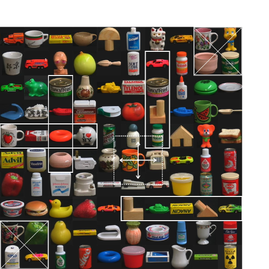
The agent earns a reward of 100 when an exit is reached. Any other move, including the forbidden ones, generates zero reinforcement. When the agent succeeds in escaping the maze, it arrives in a terminal state in which every move gives rise to a zero reinforcement. In this task, $\gamma$ was set to $0.9$. Note that the agent is faced with the delayed reward problem, and that it must take the distance to the two exits into consideration for choosing the most attractive one.

The maze has a ground carpeted with a color image of $1280\times 1280$ pixels that is a montage of pictures from the COIL-100 database (?). The agent does not have direct access to its $(x,y)$ position in the maze. Rather, its sensors take a picture of a surrounding portion of the ground. This portion is larger than the blank areas, which makes the input space fully observable. Importantly, the glass walls are transparent, so that the sensors also return the portions of the tapestry that are behind them. Therefore, there is no way for the agent to directly locate the walls. It is obliged to identify them as the regions of the maze in which an action does not change its location.

In this experiment, we have used color differential invariants as visual features (?). The entire tapestry includes 2298 different visual features. RLVC selected 200 features, corresponding to a ratio of $9\%$ of the entire set of possible features. The computation stopped after the generation of 84 image classifiers (i.e. when $k$ reached 84), which took 35 minutes on a 2.4GHz Pentium IV using databases of 10,000 interactions. 205 visual classes were identified. This is a small number, compared to the number of perceptual classes that would be generated by a discretization of the maze when the agent knows its $(x,y)$ position. For example, a reasonably sized $20\times 20$ grid leads to 400 perceptual classes.

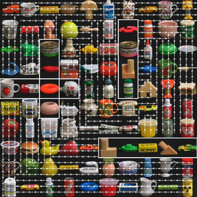
Figure 4 shows the optimal, deterministic image-to-action mapping that results from the last obtained image classifier ${\cal C}_{k}$:

$$\pi^{*}(s)=\mathop{\rm argmax}_{a\in A}Q^{*}_{k}(s,a)=Q^{\prime*}_{k}\left({\cal C}_{k}(s),a\right).$$ (15)

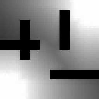
Figure 5 compares the optimal value function of the discretized problem with the one obtained through RLVC. The similarity between the two pictures indicates the soundness of our approach. Importantly, RLVC operates with neither pretreatment, nor human intervention. The agent is initially not aware of which visual features are important for its task. Moreover, the interest of selecting descriptors is clear in this application: A direct, tabular representation of the $Q$ function considering all the Boolean combinations of features would have $2^{2298}\times 4$ cells.

(a) (b)

Figure 5: (a) The optimal value function, when the agent has direct access to its $(x,y)$ position in the maze and when the set of possible locations is discretized into a $50\times 50$ grid. The brighter the location, the greater its value. (b) The final value function obtained by RLVC.

The behavior of RLVC on real-word images has also been investigated. The navigation rules were kept identical, but the tapestry was replaced by a panoramic photograph of $3041\times 384$ pixels of a subway station, as depicted in Figure 6. RLVC took 101 iterations to compute the mapping at the right of Figure 6. The computation time was 159 minutes on a 2.4GHz Pentium IV using databases of 10,000 interactions. 144 distinct visual features were selected among a set of 3739 possible ones, generating a set of 149 visual classes. Here again, the resulting classifier is fine enough to obtain a nearly optimal image-to-action mapping for the task.

(a)		(b)

Figure 6: (a) A navigation task with a real-world image, using the same conventions than Figure 3. (b) The deterministic image-to-action mapping computed by RLVC.

3.6 Related Work

RLVC can be thought of as performing adaptive discretization of the visual space on the basis of the presence of visual features. Previous reinforcement learning algorithms that exploit the presence of perceptual features in various contexts are now discussed.

3.6.1 Perceptual Aliasing

As explained above, the incremental selection of a set of informative visual features necessarily leads to temporary perceptual aliasing, which RLVC tries to remove. More generally, perceptual aliasing occurs whenever an agent cannot always take the right on the basis of its percepts.

Early work in reinforcement learning has tackled this general problem in two distinct ways: Either the agent identifies and then avoids states where perceptual aliasing occurs (as in the Lion algorithm, see ?), or it tries to build a short-term memory that will allow it to remove the ambiguities on its percepts (as in the predictive distinctions approach, see ?). Very sketchily, these two algorithms detect the presence of perceptual aliasing through an analysis of the sign of $Q$-learning updates. The possibility of managing a short-term memory has led to the development of the Partially Observable Markov Decision Processes (POMDP) theory (?), in which the current state is a random variable of the percepts.

Although these approaches are closely related to the perceptual aliasing RLVC temporarily introduces, they do not consider the exploitation of perceptual features. Indeed, they tackle a structural problem in a given control task, and, as such, they assume that perceptual aliasing cannot be removed. As a consequence, these approaches are orthogonal to our research interest, since the ambiguities RLVC generates can be removed by further refining the image classifier. In fact, the techniques above tackle a lack of information inherent to the used sensors, whereas our goal is to handle a surplus of information related to the high redundancy of visual representations.

3.6.2 Adaptive Resolution in Finite Perceptual Spaces

RLVC performs an adaptive discretization of the perceptual space through an autonomous, task-driven, purposive selection of visual features. Work in RL that incrementally partitions a large (either discrete or continuous) perceptual space into a piecewise constant value function is usually referred to as adaptive-resolution techniques. Ideally, regions of the perceptual space with a high granularity should only be present where they are needed, while a lower resolution should be used elsewhere. RLVC is such an adaptive-resolution algorithm. We now review several adaptive-resolution methods that have been previously proposed for finite perceptual spaces.

The idea of adaptive-resolution techniques in reinforcement learning goes back to the G Algorithm (?), and has inspired the other approaches that are discussed below. The G Algorithm considers perceptual spaces that are made up of fixed-length binary numbers. It learns a decision tree that tests the presence of informative bits in the percepts. This algorithm uses a Student’s $t$-test to determine if there is some bit $b$ in the percepts that is mapped to a given leaf, such that the state-action utilities of states in which $b$ is set are significantly different from the state-action utilities of states in which $b$ is unset. If such a bit is found, the corresponding leaf is split. The process is repeated for each leaf. This method is able to learn compact representations, even though there is a large number of irrelevant bits in the percepts. Unfortunately, when a region is split, all the information associated with that region is lost, which makes for very slow learning. Concretely, the G Algorithm can solve a task whose perceptual space contains $2^{100}$ distinct percepts, which corresponds to the set of binary numbers with a length of $100$ bits.

McCallum’s U-Tree algorithm builds upon this idea by combining a “selective attention” mechanism inspired by the G Algorithm with a short-term memory that enables the agent to deal with partially observable environments (?). Therefore, McCallum’s algorithms are a keystone in reinforcement learning, as they unify the G Algorithm (?) with Chrisman’s predictive distinctions (?).

U-Tree incrementally grows a decision tree through Kolmogorov-Smirnov tests. It has succeeded at learning behaviors in a driving simulator. In this simulator, a percept consists of a set of 8 discrete variables whose variation domains contain between 2 and 6 values, leading to a perceptual space with $2,592$ possible percepts. Thus, the size of the perceptual space is much smaller than a visual space. However, this task is difficult because the “physical” state space is only partially observable through the perceptual space: The driving task contains $21,216$ physical states, which means that several physical states requiring different reactions can be mapped to the same percept through the sensors of the agent. U-Tree resolves such ambiguities on the percepts by testing the presence of perceptual features in the percepts that have been encountered previously in the history of the system. To this end, U-Tree manages a short-term memory. In this paper, partially observable environments are not considered. Our challenge is rather to deal with huge visual spaces, without hand-tuned pre-processing, which is in itself a difficult, novel research direction.

3.6.3 Adaptive Resolution in Continuous Perceptual Spaces

It is important to notice that all the methods for adaptive resolution in large-scale, finite perceptual spaces use a fixed set of perceptual features that is hard-wired. This has to be distinguished from RLVC that samples visual features from a possibly infinite visual feature space (e.g. the set of visual features is infinite), and that makes no prior assumptions about the maximum number of useful features. From this point of view, RLVC is closer to adaptive-resolution techniques for continuous perceptual spaces. Indeed, these techniques dynamically select new relevant features from a whole continuum.

The first adaptive-resolution algorithm for continuous perceptual spaces is the Darling algorithm (?). This algorithm, just like all the current algorithms for continuous adaptive resolution, splits the perceptual space using thresholds. For this purpose, Darling builds a hybrid decision tree that assigns a label to each point in the perceptual space. Darling is a fully on-line and incremental algorithm that is equipped with a forgetting mechanism that deletes outdated interactions. It is however limited to binary reinforcement signals, and it only takes immediate reinforcements into account, so that Darling is much closer to supervised learning than to reinforcement learning.

The Parti-Game algorithm (?) produces goal-directed behaviors in continuous perceptual spaces. Parti-Game also splits regions where it deems it important, using a game-theoretic approach. Moore and Atkeson show that Parti-Game can learn competent behavior in a variety of continuous domains. Unfortunately, the approach is currently limited to deterministic domains where the agent has a greedy controller and where the goal state is known. Moreover, this algorithm searches for any solution to a given task, and does not try to find the optimal one.

The Continuous U-Tree algorithm is an extension of U-Tree that is adapted to continuous perceptual spaces (?). Just like Darling, Continuous U-Tree incrementally builds a decision tree that splits the perceptual space into a finite set of hypercubes, by testing thresholds. Kolmogorov-Smirnov and sum-of-squared-errors are used to determine when to split a node in the decision tree. Pyeatt and Howe (?) analyze the performance of several splitting criteria for a variation of Continuous U-Tree. They conclude that Student’s $t$-test leads to the best performance, which motivates the use of this statistical test in RLVC (cf. Section 3.4).

Munos and Moore (?) have proposed Variable Resolution Grids. Their algorithm assumes that the perceptual space is a compact subset of Euclidean space, and begins with a coarse, grid-based discretization of the state space. In contrast with the other abstract algorithms in this section, the value function and policy vary linearly within each region. Munos and Moore use Kuhn triangulation as an efficient way to interpolate the value function within regions. The algorithm refines its approximation by refining cells according to a splitting criterion. Munos and Moore explore several local heuristic measures of the importance of splitting a cell including the average of corner-value differences, the variance of corner-value differences, and policy disagreement. They also explore global heuristic measures involving the influence and variance of the approximated system. Variable Resolution Grids are probably the most advanced adaptive-resolution algorithm available so far.

3.6.4 Discussion

To summarize, several algorithms that are similar in spirit to RLVC have been proposed over the years. Nevertheless, our work appears to be the first that can learn direct image-to-action mappings through reinforcement learning. Indeed, none of the reinforcement learning methods above combines all the following desirable properties of RLVC: (1) The set of relevant perceptual features is not chosen a priori by hand, as the selection process is fully automatic and does not require any human intervention; (2) visual perceptual spaces are explicitly considered through appearance-based visual features; and (3) the highly informative perceptual features can be drawn out of a possibly infinite set.

These advantages of RLVC are essentially due to the fact that the candidate visual features are not selected only because they are informative: They are also ranked according to an information-theoretic measure inspired by decision tree induction (?). Such a ranking is required, as vision-for-action tasks induce a large number of visual features (a typical image contains about a thousand of them). This kind of criterion that ranks features, though already considered in Variable Resolution Grids (?), seems to be new in discrete perceptual spaces.

RLVC is defined independently of any fixed RL algorithm, which is similar in spirit to Continuous U-Tree (?), with the major exception that RLVC deals with Boolean features, whereas Continuous U-Tree works in a continuous input space. Furthermore, the version of RLVC presented in this paper uses a variance-reduction criterion for ranking the visual features. This criterion, though already considered in Variable Resolution Grids, seems to be new in discrete perceptual spaces.

4 Compacting Visual Policies

As written in Section 1.4.2, this original version of RLVC is subject to overfitting (?). A simple heuristic to avoid the creation of too many visual classes is simply to bound the number of visual classes that can be refined at each stage of the algorithm, since splitting one visual class potentially has an impact on the Bellman residuals of all the visual classes. In practice, we first try to split the classes that have the most samples before considering the others, since there is more evidence of variance reduction for the first. In our tests, we systematically apply this heuristics. However, it is often insufficient if taken alone.

4.1 Equivalence Relations in Markov Decision Processes

Since we apply an embedded RL algorithm at each stage $k$ of RLVC, properties like the optimal value function $V^{*}_{k}(\cdot)$, the optimal state-action value function $Q^{*}_{k}(\cdot,\cdot)$ and the optimal control policy $\pi^{*}_{k}(\cdot)$ are known for each mapped MDP ${\cal M}_{k}$. Using those properties, it is easy to define a whole range of equivalence relations between the visual classes. For instance, given a threshold $\varepsilon\in\mathbb{R}^{+}$, we list hereunder three possible equivalence relations for a pair of visual classes $(V,V^{\prime})$:

Optimal Value Equivalence:

$|V^{*}_{k}(V)-V^{*}_{k}(V^{\prime})|\leq\varepsilon.$

Optimal Policy Equivalence:

$|V^{*}_{k}(V)-Q^{*}_{k}(V^{\prime},\pi^{*}_{k}(V))|\leq\varepsilon~{}\wedge$
$|V^{*}_{k}(V^{\prime})-Q^{*}_{k}(V,\pi^{*}_{k}(V^{\prime}))|\leq\varepsilon.$

Optimal State-Action Value Equivalence:

$(\forall a\in A)\ |Q^{*}_{k}(V,a)-Q^{*}_{k}(V^{\prime},a)|\leq\varepsilon.$

We therefore propose to modify RLVC so that, periodically, visual classes that are equivalent with respect to one of those criteria are merged together. We have experimentally observed that the conjunction of the first two criteria tends to lead to the best performance. This way, RLVC alternatively splits and merges visual classes. The compaction phase should not be done too often, in order to allow exploration. To the best of our knowledge, this possibility has not been investigated yet in the framework of adaptive-resolution methods in reinforcement learning.

In the original version of RLVC, the visual classes correspond to the leaves of a decision tree. When using decision trees, the aggregation of visual classes can only be achieved by starting from the bottom of the tree and recursively collapsing leaves, until dissimilar leaves are found. This operation is very close to post-pruning in the framework of decision trees for machine learning (?). In practice, this means that classes that have similar properties, but that can only be reached from one another by making a number of hops upwards then downwards, are extremely unlikely to be matched. This greatly reduces the interest of exploiting the equivalence relations.

This drawback is due to the rather limited expressiveness of decision trees. In a decision tree, each visual class corresponds to a conjunction of visual feature literals, which defines a path from the root of the decision tree to one leaf. To take full advantage of the equivalence relations, it is necessary to associate, to each visual class, an arbitrary union of conjunctions of visual features. Indeed, when exploiting the equivalence relations, the visual classes are the result of a sequence of conjunctions (splitting) and disjunctions (aggregation). Thus, a more expressive data structure that would be able to represent general, arbitrary Boolean combinations of visual features is required. Such a data structure is introduced in the next section.

4.2 Using Binary Decision Diagrams

The problem of representing general Boolean functions has been extensively studied in the field of computer-aided verification, since they can abstract the behavior of logical electronic devices. In fact, a whole range of methods for representing the state space of richer and richer domains have been developed over the last few years, such as Binary Decision Diagram (BDD) (?), Number and Queue Decision Diagrams (?), Upward Closed Sets (?) and Real Vector Automata (?).

In our framework, BDD is a particularly well-suited tool. It is a acyclic graph-based symbolic representation for encoding arbitrary Boolean functions, and has had much success in the field of computer-aided verification (?). A BDD is unique when the ordering of its variables is fixed, but different variable orderings can lead to different sizes of the BDD, since some variables can be discarded by the reordering process. Although the problem of finding the optimal variable ordering is coNP-complete (?), automatic heuristics can in practice find orderings that are close to optimal. This is interesting in our case, since reducing the size of the BDD potentially discards irrelevant variables, which correspond to removing useless visual features.

4.3 Modifications to RLVC

To summarize, this extension to RLVC does not use decision trees anymore, but assigns one BDD to each visual class. Two modifications are to be applied to Algorithm 1:

1. The operation of refining, with a visual feature $f$, a visual class $V$ that is labeled by the BDD ${\cal B}(V)$, consists in replacing $V$ by two new visual classes $V_{1}$ and $V_{2}$ such that ${\cal B}(V_{1})={\cal B}(V)\wedge f$ and ${\cal B}(V_{2})={\cal B}(V)\wedge\neg f$.

2. Given an equivalence relation, the $\mbox{\tt post-process}({\cal C}_{k})$ operation consists in merging the equivalent visual classes. To merge a pair of visual classes $(V_{1},V_{2})$, $V_{1}$ and $V_{2}$ are deleted, and a new visual class $V$ such that ${\cal B}(V)={\cal B}(V_{1})\vee{\cal B}(V_{2})$ is added. Every time a merging operation takes place, it is advised to carry on variable reordering, to minimize the memory requirements.

4.4 Experiments

Figure 7: The Montefiore campus at Liège. Red spots corresponds to the places between which the agent moves. The agent can only follow the links between the different spots. Its goal is to enter the Montefiore Institute, that is labeled by a red cross, where it gets a reward of $+100$.

Figure 8: One of the optimal, deterministic control policies for the Montefiore navigation task. For each state, we have indicated the optimal action (the letter “F” stands for “move forward”, “R” for “turn right” and “L” for “turn left”). This policy has been obtained by applying a standard RL algorithm to the scenario in which the agent has direct access to the $(p,d)$ information.

Figure 9: The percepts of the agent. Four possible different percepts are shown, that correspond to the location and viewing direction marked in yellow on the top image.

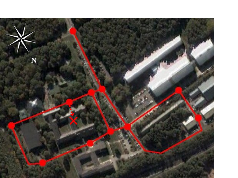
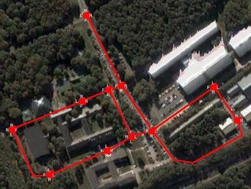
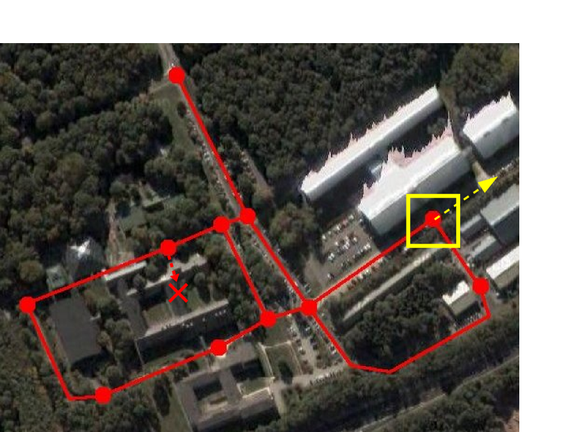
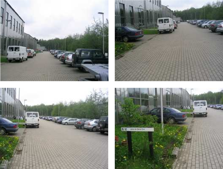
We have applied the modified version of RLVC to another simulated navigation task. In this task, the agent moves between 11 spots of the campus of the University of Liège (cf. Figure 7). Every time the agent is at one of the 11 locations, its body can aim at four possible orientations: North, South, West, East. The state space is therefore of size $11\times 4=44$. The agent has three possible actions: Turn left, turn right, go forward. Its goal is to enter a specific building, where it will obtain a reward of $+100$. Turning left or right induces a penalty of $-5$, and moving forward, a penalty of $-10$. The discount factor $\gamma$ is set to $0.8$. The optimal control policy is not unique: One of them is depicted on Figure 8.

The agent does not have direct access to its position and its orientation. Rather, it only perceives a picture of the area that is in front of it (cf. Figure 9). Thus, the agent has to connect an input image to the appropriate reaction without explicitly knowing its geographical localization. For each possible location and each possible viewing direction, a database of 24 images of size $1024\times 768$ with significant viewpoint changes has been collected. Those 44 databases have been randomly divided into a learning set of 18 images and a test set of 6 images. In our experimental setup, both versions of RLVC learn an image-to-action mapping using interactions that only contain images from the learning set. Images from the test set are used to assess the accuracy of the learned visual control policies.

The SIFT keypoints have been used as visual features (?). Thresholding on a Mahalanobis distance gave rise to a set of 13,367 distinct features. Both versions of RLVC have been applied on a static database of 10,000 interactions that has been collected using a fully randomized exploration policy. The same database is used throughout the entire algorithm, and this database only contains images that belong to the learning set.

Figure 10: Comparison of the error rates between the basic and extended versions of RLVC. The error of the computed policy as a function of the step counter $k$ on the images of the learning set (resp. test set) is reported on the left of the figure (resp. on the right).

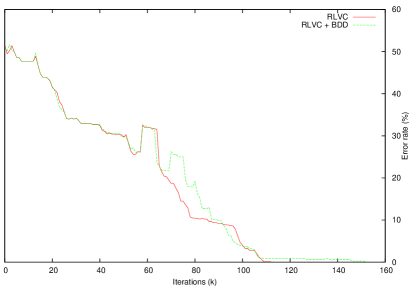
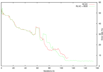
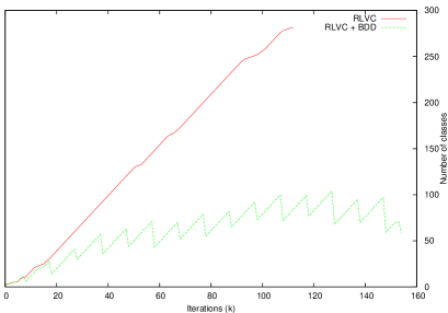
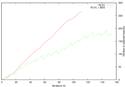
The results of the basic version of RLVC and of the version that is extended by BDDs are reported in Figures 10 and 11. The original version of RLVC has identified 281 visual classes by selecting 264 SIFT features. The error rate on the computed visual policy (i.e. the proportion of sub-optimal decisions when the agent is presented all the possible stimuli) was $0.1\%$ on the learning set and $8\%$ when the images of the test set are used, with respect to the optimal policy when the agent has direct access to its position and viewing direction.

The modified version RLVC was then applied, with one compacting stage every 10 steps. The results are clearly superior. There is no error on the learning set anymore, while the error rate on the test set is $4.5\%$. The number of selected features is reduced to 171. Furthermore, the resulting number of visual classes becomes 59, instead of 281. Thus, there is a large improvement in the generalization abilities, as well as a reduction of the number of visual classes and selected features. Interestingly enough, the number of visual classes (59) is very close to the number of physical states (44), which tends to indicate that the algorithm starts to learn a physical interpretation for its percepts.

To summarize, compacting visual policies is probably a required step to deal with realistic visual tasks, if an iterative splitting process is applied. The price to pay is of course a higher computational cost. Future work will focus on a theoretical justification of the used equivalence relations. This implies bridging the gap with the theory of MDP minimization (?).

5 Learning Spatial Relationships

As motivated in the Introduction (Section 1.4.3), we propose to extend RLVC by constructing a hierarchy of spatial arrangements of individual point features (?). The idea of learning models of spatial combinations of features takes its roots in the seminal paper by Fischler and Elschlager (?) about pictorial structures, which are collections of rigid parts arranged in deformable configurations. This idea has become increasingly popular in the computer vision community over the 90’s, and has led to a large literature about the modeling and the detection of objects (?, ?, ?). Crandall and Huttenlocher (?) provide pointers to recent resources. Among such recent techniques, Scalzo and Piater (?) propose to build a probabilistic hierarchy of visual features that is represented through an acyclic graph. They detect the presence of such a model through Nonparametric Belief Propagation (?). Other graphical models have been proposed for representing articulated structures, such as pictorial structures (?, ?). Similarly, the constellation model represents objects by parts, each modeled in terms of both shape and appearance by Gaussian probability density functions (?).

Figure 11: Comparison of the number of generated classes and selected visual features between the basic and extended versions of RLVC. The number of visual classes (resp. selected features) as a function of the step counter $k$ is plotted on the left of the figure (resp. on the right).

Our work contrasts with these approaches in that the generation of so-called composite features is driven by the task to be solved. This should be distinguished from the techniques for unsupervised learning of composite features, since the additional information that is embedded inside the reinforcement signal drives the generation of composite features by focusing the exploration on task-relevant spatial arrangements.

In this extension of RLVC, a hierarchy of visual features is built simultaneously with the image classifier. As soon as no sufficiently informative visual feature can be extracted, the algorithm tries to combine two visual features in order to construct a higher level of abstraction, which is hopefully more distinctive and more robust to noise. This extension to RLVC assumes the co-existence of two different kinds of visual features:

Primitive Features:

They correspond to the individual point features, i.e. to the local-appearance descriptors (cf. Section 1.3).

Composite Features:

They consist of spatial combinations of lower-level visual features. There is no a priori bound on the maximal height of the hierarchy. Therefore, a composite feature can be potentially combined with a primitive feature, or with a composite feature.

5.1 Detection of Visual Features

A natural way to represent such a hierarchy is to use a directed acyclic graph $G=(V,E)$, in which each vertex $v\in V$ corresponds to a visual feature, and in which each edge $(v,v^{\prime})\in E$ models the fact that $v^{\prime}$ is a part of the composite feature $v$. Thus, $G$ must be binary, i.e. any vertex should have either no child, or exactly two children. The set $V_{P}$ of the leaves of $G$ corresponds to the set of primitive features, while the set $V_{C}$ of its internal vertexes represents the set of composite features.

Each leaf vertex $v_{P}\in V_{P}$ is annotated with a local descriptor $D(v_{P})$. Similarly, each internal vertex $v_{C}\in V_{C}$ is annotated with constraints on the relative position between its parts. In this work, we consider only constraints on the distances between the constituent visual features of the composite features, and we assume that they should be distributed according to a Gaussian law ${\cal G}(\mu,\sigma)$ of mean $\mu$ and standard deviation $\sigma$. Evidently, richer constraints could be used, such as taking the relative orientation or the scaling factor between the constituent features into consideration, which would require the use of multivariate Gaussians.

More precisely, let $v_{C}$ be a composite feature, the parts of which are $v_{1}$ and $v_{2}$. In order to trigger the detection of $v_{C}$ in an image $s$, there should be an occurrence of $v_{1}$ and an occurrence of $v_{2}$ in $s$ such that their relative Euclidean distance has a sufficient likelihood $\nu$ of being generated by a Gaussian of mean $\mu(v_{C})$ and standard deviation $\sigma(v_{C})$. To ensure symmetry, the location of the composite feature is then taken as the midpoint between the locations of $v_{1}$ and $v_{2}$.

The occurrences of a visual feature $v$ in a percept $s$ can be found using the recursive Algorithm 5. Of course, at steps 6 and 7 of Algorithm 4, the test “does $s_{t}$ exhibit $v$?” can be rewritten as a function of Algorithm 5, by checking if $\mbox{\tt occurrences}(v,s_{t})\not=\emptyset$.

Algorithm 5 — Detecting Composite Features

1:  $\mbox{\tt occurrences}(v,s)$ :–

2:     if $v$ is primitive then

3:        return {$(x,y)\mid$ $(x,y)$ is an interest point of $s$, the local descriptor of which corresponds to $D(v)$}

4:     else

5:        $O\leftarrow\{\}$

6:        $O_{1}\leftarrow\mbox{\tt occurrences}(\mbox{\tt subfeature}_{1}(v),s)$

7:        $O_{2}\leftarrow\mbox{\tt occurrences}(\mbox{\tt subfeature}_{2}(v),s)$

8:        for all $(x_{1},y_{1})\in O_{1}$ and $(x_{2},y_{2})\in O_{2}$ do

9:           $d\leftarrow\sqrt{(x_{2}-x_{1})^{2}+(y_{2}-y_{1})^{2}}$

10:           if ${\cal G}(d-\mu(v),\sigma(v))\geq\nu$ then

11:              $O\leftarrow O\cup\{((x_{1}+x_{2})/2,(y_{1}+y_{2})/2)\}$

12:           end if

13:        end for

14:        return $O$

15:     end if

5.2 Generation of Composite Features

The cornerstone of this extension to RLVC is the way of generating composite features. The general idea behind our algorithm is to accumulate statistical evidence from the relative positions of the detected visual features in order to find “conspicuous coincidences” of visual features. This is done by providing a more evolved implementation of $\mbox{\tt generator}(s_{1},\ldots,s_{n})$ than the one of Algorithm 3.

5.2.1 Identifying Spatial Relations

We first extract the set $F$ of all the (primitive or composite) features that occur within the set of provided images $\{s_{1},\ldots,s_{n}\}$:

$$F=\left\{v\in V\mid(\exists i)~{}s_{i}\mbox{~{}exhibits~{}}v\right\}.$$ (16)

We identify the pairs of visual features the occurrences of which are highly correlated within the set of provided images $\{s_{1},\ldots,s_{n}\}$. This simply amounts to counting the number of co-occurrences for each pair of features in $F$, then only keeping the pairs the corresponding count of which exceeds a fixed threshold.

Let now $v_{1}$ and $v_{2}$ be two features that are highly correlated. A search for a meaningful spatial relationship between $v_{1}$ and $v_{2}$ is then carried out in the images $\{s_{1},\ldots,s_{n}\}$ that contain occurrences of both $v_{1}$ and $v_{2}$. For each such co-occurrence, we accumulate in a set $\Lambda$ the distances between the corresponding occurrences of $v_{1}$ and $v_{2}$. Finally, a clustering algorithm is applied on the distribution $\Lambda$ in order to detect typical distances between $v_{1}$ and $v_{2}$. For the purpose of our experiments, we have used hierarchical clustering (?). For each cluster, a Gaussian is fitted by estimating a mean value $\mu$ and a standard deviation $\sigma$. Finally, a new composite feature $v_{C}$ is introduced in the feature hierarchy, that has $v_{1}$ and $v_{2}$ as parts and such that $\mu(v_{C})=\mu$ and $\sigma(v_{C})=\sigma$.

In summary, in Algorithm 1, we replace the call to Algorithm 3 by a call to Algorithm 6.

Algorithm 6 — Generation of Composite Features

1:  $\mbox{\tt generator}(\{s_{1},\ldots,s_{n}\})$ :–

2:     $F=\left\{v\in V\mid(\exists i)~{}s_{i}\mbox{~{}exhibits~{}}v\right\}$

3:     $F^{\prime}=\{\}$

4:     for all $(v_{1},v_{2})\in F\times F$ do

5:        if enough co-occurrences of $v_{1}$ and $v_{2}$ in $\{s_{1},\ldots,s_{n}\}$ then

6:           $\Lambda\leftarrow\{\}$

7:           for all $i\in\{1,\ldots,n\}$ do

8:              for all occurrences $(x_{1},y_{1})$ of $v_{1}$ in $s_{i}$ do

9:                 for all occurrences $(x_{2},y_{2})$ of $v_{2}$ in $s_{i}$ do

10:                    $\Lambda\leftarrow\Lambda\cup\{\sqrt{(x_{2}-x_{1})^{2}+(y_{2}-y_{1})^{2}}\}$

11:                 end for

12:              end for

13:           end for

14:           Apply a clustering algorithm on $\Lambda$

15:           for each cluster $C=\{d_{1},\ldots d_{m}\}$ in $\Lambda$ do

16:              $\mu=\mathop{\rm mean}(C)$

17:              $\sigma=\mathop{\rm stddev}(C)$

18:              Add to $F^{\prime}$ a composite feature $v_{C}$ composed of $v_{1}$ and $v_{2}$, annotated with a mean $\mu$ and a standard deviation $\sigma$

19:           end for

20:        end if

21:     end for

22:     return $F^{\prime}$

5.2.2 Feature Validation

Algorithm 6 can generate several composite features for a given visual class $V_{k,i}$. However, at the end of Algorithm 4, at most one generated composite feature is to be kept. It is important to notice that the performance of the clustering method is not critical for our purpose. Indeed, irrelevant spatial combinations are automatically discarded, thanks to the variance-reduction criterion of the feature selection component. In fact, the reinforcement signal helps to direct the search for a good feature, which is an advantage over unsupervised methods of building feature hierarchies.

5.3 Experiments

We demonstrate the efficacy of our algorithms on a version of the classical “Car on the Hill” control problem (?), where the position and velocity information is presented to the agent visually.

In this episodic task, a car (modeled by a mass point) is riding without friction on a hill, the shape of which is defined by the function:

$$H(p)=\left\{\begin{array}[]{ll}p^{2}+p&\mbox{if~{}}p<0,\\ p/\sqrt{1+5p^{2}}&\mbox{if~{}}p\geq 0.\end{array}\right.$$

The goal of the agent is to reach as fast as possible the top of the hill, i.e. a location such that $p\geq 1$. At the top of the hill, the agent obtains a reward of 100. The car can thrust left or right with an acceleration of $\pm 4$ Newtons. However, because of gravity, this acceleration is insufficient for the agent to reach the top of the hill by always thrusting toward the right. Rather, the agent has to go left for while, hence acquiring potential energy by going up the left side of the hill, before thrusting rightward. There are two more constraints: The agent is not allowed to reach locations such that $p<-1$, and a velocity greater than 3 in absolute value leads to the destruction of the car.

Figure 12: The “Car on the Hill” control problem.

5.3.1 Formal Definition of the Task

Formally, the set of possible actions is $A=\{-4,4\}$, while the state space is $S=\{(p,s)\mid|p|\leq 1\wedge|s|\leq 3\}.$ The system has the following continuous-time dynamics:

$$\dot{p} = s$$

$$\dot{s} = \frac{a}{M\sqrt{1+H^{\prime}(p)^{2}}}-\frac{gH^{\prime}(p)}{1+H^{\prime}(p)^{2}},$$

where $a\in A$ is the thrust acceleration, $H^{\prime}(p)$ is the first derivative of $H(p)$, $M=1$ is the mass of the car, and $g=9.81$ is the acceleration due to gravity. These continuous-time dynamics are approximated by the following discrete-time state update rule:

$$s_{t+1} = s_{t}+h\dot{p}_{t}+h^{2}\dot{s}_{t}/2$$

$$s_{t+1} = \dot{p}_{t}+h\dot{s}_{t},$$

where $h=0.1$ is the integration time step. The reinforcement signal is defined through this expression:

$${\cal R}((s_{t},s_{t}),a)=\left\{\begin{array}[]{ll}100&\mbox{if~{}}s_{t+1}\geq 1\wedge|s_{t+1}|\leq 3,\\ 0&\mbox{otherwise}.\end{array}\right.$$

In our setup, the discount factor $\gamma$ was set to $0.75$.

This definition is actually a mix of two coexistent formulations of the “Car on the Hill” task (?, ?). The major differences with the initial formulation of the problem (?) is that the set of possible actions is discrete, and that the goal is at the top of the hill (rather than on a given area of the hill), just like in the definition from Ernst et al. (?). To ensure the existence of an interesting solution, the velocity is required to remain less than 3 (instead of 2), and the integration time step is set to $h=0.1$ (instead of $0.01$).

5.3.2 Inputs of the Agent

In previous work (?, ?), the agent was always assumed to have direct access to a numerical measure of its position and velocity. The only exception is Gordon’s work in which a visual, low-resolution representation of the global scene is given to the agent (?). In our experimental setup, the agent is provided with two cameras, one looking at the ground underneath, the second at a velocity gauge. This way, the agent cannot directly know its current position and velocity, but has to suitably interpret its visual inputs to derive them.

Some examples of the pictures the sensors can return are presented in Figure 13. The ground is carpeted with a color image of $1280\times 128$ pixels that is a montage of pictures from the COIL-100 database (?). It is very important to notice that using individual point features is insufficient for solving this task, since the set of features in the pictures of the velocity gauge are always the same. To know its velocity, the agent has to generate composite features sensitive to the distance of the primitive features on the cursor with respect to the primitive features on the digits.

(a)

(b)

Figure 13: (a) Visual percepts corresponding to pictures of the velocity gauge when $s=-3$, $s=0.5$ and $s=1.5$. (b) Visual percepts returned by the position sensor. The region framed with a white rectangle corresponds to the portion of the ground that is returned by the sensor when $p=0.1$. This portion slides back and forth as the agent moves.

5.3.3 Results

In this experimental setup, we used color differential invariants (?) as primitive features. Among all the possible visual inputs (both for the position and the velocity sensors), there were 88 different primitive features. The entire image of the ground includes 142 interest points, whereas the images of the velocity gauge include about 20 interest points.

The output of RLVC is a decision tree that defines 157 visual classes. Each internal node of this tree tests the presence of one visual feature, taken from a set of 91 distinct, highly discriminant features selected by RLVC. Among the 91 selected visual features, there were 56 primitive and 26 composite features. Two examples of composites features that were selected by RLVC are depicted in Figure 15. The computation stopped after $k=38$ refinement steps in Algorithm 1.

(a)

(b)

Figure 14: (a) The optimal value function, when the agent has a direct access to its current $(p,s)$ state, and when the input space is discretized in a $13\times 13$ grid. The brighter the location, the greater its value. (b) The value function obtained by RLVC.

Figure 15: Two composite features that were generated, in yellow. The primitive features of which they are composed are marked in yellow. The first feature triggers for velocities around 0, whereas the second triggers around $-2$.

Figure 16: Evolution of the number of times the goal was missed over the iterations of RLVC.

Figure 17: Evolution of the mean lengths of the successful trials over the iterations of RLVC.

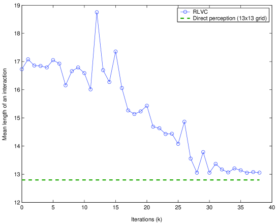
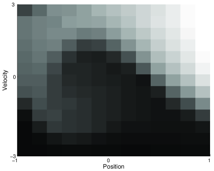
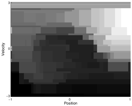
To show the efficacy of our method, we compare its performance with the scenario in which the agent has a direct perception of its current $(p,s)$ state. In the latter scenario, the state space was discretized in a grid of $13\times 13$ cells. The number 13 was chosen since it approximately corresponds to the square root of 157, the number of visual classes that were produced by RLVC. This way, RL is provided an equivalent number of perceptual classes in the two scenarios. Figure 14 compares the optimal value function of the direct-perception problem with the one obtained through RLVC. Here also, the two pictures are very similar, which indicates the soundness of our approach.

We have also evaluated the performance of the optimal image-to-action mapping

$$\pi^{*}=\mathop{\rm argmax}_{a\in A}Q^{*}((p,s),a)$$ (17)

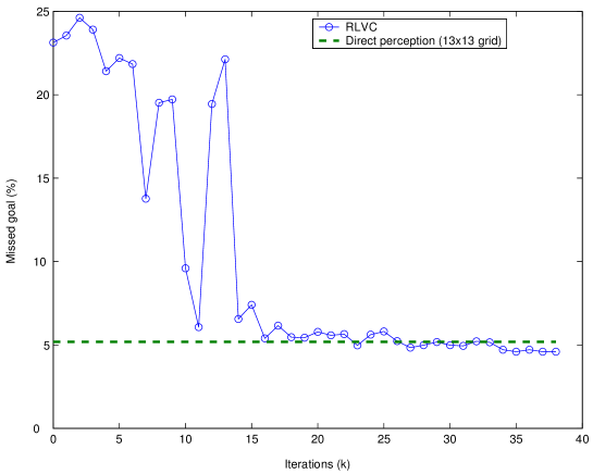
obtained through RLVC. For this purpose, the agent was placed randomly on the hill, with an initial velocity of 0. Then, it used the mapping $\pi^{*}$ to choose an action, until it reached a final state. A set of 10,000 such trials were carried out at each step $k$ of Algorithm 1. Figure 16 compares the proportion of trials that missed the goal (either because of leaving the hill on the left, or because of acquiring a too high velocity) in RLVC and in the direct-perception problem. When $k$ became greater than 27, the proportion of missed trials was always smaller in RLVC than in the direct-perception problem. This advantage in favor of RLVC is due to the adaptive nature of its discretization. Figure 17 compares the mean lengths of the successful trials. The mean length of RLVC trials clearly converges to that of the direct-perception trials, while staying slightly larger.

To conclude, RLVC achieves a performance close to the direct-perception scenario. However, the mapping built by RLVC directly links visual percepts to the appropriate actions, without considering explicitly the physical variables.

6 Summary

This paper introduces Reinforcement Learning of Visual Classes (RLVC). RLVC is designed to learn mappings that directly connect visual stimuli to output actions that are optimal for the surrounding environment. The framework of RLVC is general, in the sense that it can be applied to any problem that can be formulated as a Markov decision problem.

The learning process behind our algorithms is closed-loop and flexible. The agent takes lessons from its interactions with the environment, according to the purposive vision paradigm. RLVC focuses the attention of an embedded reinforcement learning algorithm on highly informative and robust parts of the inputs by testing the presence or absence of local descriptors at the interest points of the input images. The relevant visual features are incrementally selected in a sequence of attempts to remove perceptual aliasing: The discretization process targets zero Bellman residuals and is inspired from supervised learning algorithms for building decision trees. Our algorithms are defined independently of any interest point detector (?) and of any local description technique (?). The user may choose these two components as he sees fit.

Techniques for fighting overfitting in RLVC have also been proposed. The idea is to aggregate visual classes that share similar properties with respect to the theory of Dynamic Programming. Interestingly, this process enhances the generalization abilities of the learned image-to-action mapping, and reduces the number of visual classes that are built.

Finally, an extension of RLVC is introduced that allows the closed-loop, interactive and purposive learning of a hierarchy of geometrical combinations of visual features. This is to contrast to most of the prior work on the topic, that uses either a supervised or unsupervised framework (?, ?, ?, ?). Besides the novelty of the approach, we have shown its practical value in visual control tasks in which the information provided by the individual point features alone is insufficient for solving the task. Indeed, spatial combinations of visual features are more informative and more robust to noise.

7 Future Work

The area of applications of RLVC is wide, since nowadays robotic agents are often equipped with CCD sensors. Future research includes the demonstration of the applicability of our algorithms in a reactive robotic application, such as grasping objects by combining visual and haptic feedback (?). This necessitates the extension of our techniques to continuous action spaces, for which no fully satisfactory solutions exist to date. RLVC could also be potentially be applied to Human-Computer Interaction, as the actions need not be physical actions.

The closed-loop learning of a hierarchy of visual feature also raises interesting research directions. For example, the combination of RLVC with techniques for disambiguating between aliased percepts using a short-term memory (?) could solve visual tasks in which the percepts of the agent alone do not provide enough information for solving the task. Likewise, the unsupervised learning of other kinds of geometrical models (?) could potentially be embedded in RLVC. On the other hand, spatial relationships do not currently take into consideration the relative angles between the parts of a composite feature. Doing so would further increase the discriminative power of the composite features, but requires non-trivial techniques for clustering in circular domains.

References

- Aloimonos Aloimonos, Y. (1990). Purposive and qualitative active vision. In Proc. of the 10th International Conference on Pattern Recognition, pp. 436–460.
- Amit & Kong Amit, Y., & Kong, A. (1996). Graphical templates for model registration. IEEE Transactions on Pattern Analysis and Machine Intelligence, 18(3), 225–236.
- Asada, Noda, Tawaratsumida, & Hosoda Asada, M., Noda, S., Tawaratsumida, S., & Hosoda, K. (1994). Vision-based behavior acquisition for a shooting robot by using a reinforcement learning. In Proc. of IAPR/IEEE Workshop on Visual Behaviors, pp. 112–118.
- Bagnell & Schneider Bagnell, J., & Schneider, J. (2001). Autonomous helicopter control using reinforcement learning policy search methods. In Proc. of the International Conference on Robotics and Automation. IEEE.
- Barto, Sutton, & Anderson Barto, A., Sutton, R., & Anderson, C. (1983). Neuronlike adaptive elements that can solve difficult learning control problems. IEEE Transactions on Systems, Man and Cybernetics, 13(5), 835–846.
- Bellman Bellman, R. (1957). Dynamic Programming. Princeton University Press.
- Bertsekas & Tsitsiklis Bertsekas, D., & Tsitsiklis, J. (1996). Neuro-Dynamic Programming. Athena Scientific.
- Boigelot Boigelot, B. (1999). Symbolic Methods for Exploring Infinite State Spaces. Ph.D. thesis, University of Liège, Liège (Belgium).
- Boigelot, Jodogne, & Wolper Boigelot, B., Jodogne, S., & Wolper, P. (2005). An effective decision procedure for linear arithmetic with integer and real variables. ACM Transactions on Computational Logic (TOCL), 6(3), 614–633.
- Bouchard & Triggs Bouchard, G., & Triggs, B. (2005). Hierarchical part-based visual object categorization. In IEEE Conference on Computer Vision and Pattern Recognition, Vol. 1, pp. 710–715, San Diego (CA, USA).
- Breiman, Friedman, & Stone Breiman, L., Friedman, J., & Stone, C. (1984). Classification and Regression Trees. Wadsworth International Group.
- Bryant Bryant, R. (1986). Graph-based algorithms for boolean function manipulation. IEEE Transactions in Computers, 8(35), 677–691.
- Bryant Bryant, R. (1992). Symbolic boolean manipulation with ordered binary decision diagrams. ACM Computing Surveys, 24(3), 293–318.
- Burl & Perona Burl, M., & Perona, P. (1996). Recognition of planar object classes. In Proc. of the IEEE Conference on Computer Vision and Pattern Recognition, pp. 223–230, San Francisco (CA, USA).
- Chapman & Kaelbling Chapman, D., & Kaelbling, L. (1991). Input generalization in delayed reinforcement learning: An algorithm and performance comparisons. In Proc. of the 12th International Joint Conference on Artificial Intelligence (IJCAI), pp. 726–731, Sydney.
- Chrisman Chrisman, L. (1992). Reinforcement learning with perceptual aliasing: The perceptual distinctions approach. In National Conference on Artificial Intelligence, pp. 183–188.
- Coelho, Piater, & Grupen Coelho, J., Piater, J., & Grupen, R. (2001). Developing haptic and visual perceptual categories for reaching and grasping with a humanoid robot. Robotics and Autonomous Systems, special issue on Humanoid Robots, 37(2–3), 195–218.
- Crandall & Huttenlocher Crandall, D., & Huttenlocher, D. (2006). Weakly supervised learning of part-based spatial models for visual object recognition. In Proc. of the 9th European Conference on Computer Vision.
- Delzanno & Raskin Delzanno, G., & Raskin, J.-F. (2000). Symbolic representation of upward closed sets. In Tools and Algorithms for the Construction and Analysis of Systems, Lecture Notes in Computer Science, pp. 426–440, Berlin (Germany).
- Derman Derman, C. (1970). Finite State Markovian Decision Processes. Academic Press, New York.
- Ernst, Geurts, & Wehenkel Ernst, D., Geurts, P., & Wehenkel, L. (2003). Iteratively extending time horizon reinforcement learning. In Proc. of the 14th European Conference on Machine Learning, pp. 96–107, Dubrovnik (Croatia).
- Ernst, Geurts, & Wehenkel Ernst, D., Geurts, P., & Wehenkel, L. (2005). Tree-based batch mode reinforcement learning. Journal of Machine Learning Research, 6, 503–556.
- Felzenszwalb & Huttenlocher Felzenszwalb, P., & Huttenlocher, D. (2005). Pictorial structures for object recognition. International Journal of Computer Vision, 61(1), 55–79.
- Fergus, Perona, & Zisserman Fergus, R., Perona, P., & Zisserman, A. (2003). Object class recognition by unsupervised scale-invariant learning. In IEEE Conference on Computer Vision and Pattern Recognition, Vol. 2, pp. 264–271, Madison (WI, USA).
- Fischler & Elschlager Fischler, M., & Elschlager, R. (1973). The representation and matching of pictorial structures. IEEE Transactions on Computers, 22(1), 67–92.
- Forsyth, Haddon, & Ioffe Forsyth, D., Haddon, J., & Ioffe, S. (1999). Finding objects by grouping primitives. In Shape, Contour and Grouping in Computer Vision, pp. 302–318, London (UK). Springer-Verlag.
- Gaskett, Fletcher, & Zelinsky Gaskett, C., Fletcher, L., & Zelinsky, A. (2000). Reinforcement learning for visual servoing of a mobile robot. In Proc. of the Australian Conference on Robotics and Automation, Melbourne (Australia).
- Gibson & Spelke Gibson, E., & Spelke, E. (1983). The development of perception. In Flavell, J. H., & Markman, E. M. (Eds.), Handbook of Child Psychology Vol. III: Cognitive Development (4th edition)., chap. 1, pp. 2–76. Wiley.
- Givan, Dean, & Greig Givan, R., Dean, T., & Greig, M. (2003). Equivalence notions and model minimization in markov decision processes. Artificial Intelligence, 147(1–2), 163–223.
- Gordon Gordon, G. (1995). Stable function approximation in dynamic programming. In Proc. of the International Conference on Machine Learning, pp. 261–268.
- Gouet & Boujemaa Gouet, V., & Boujemaa, N. (2001). Object-based queries using color points of interest. In IEEE Workshop on Content-Based Access of Image and Video Libraries, pp. 30–36, Kauai (HI, USA).
- Howard Howard, R. (1960). Dynamic Programming and Markov Processes. Technology Press and Wiley, Cambridge (MA) and New York.
- Huber & Grupen Huber, M., & Grupen, R. (1998). A control structure for learning locomotion gaits. In 7th Int. Symposium on Robotics and Applications, Anchorage (AK, USA). TSI Press.
- Iida, Sugisaka, & Shibata Iida, M., Sugisaka, M., & Shibata, K. (2002). Direct-vision-based reinforcement learning to a real mobile robot. In Proc. of International Conference of Neural Information Processing Systems, Vol. 5, pp. 2556–2560.
- Jaakkola, Jordan, & Singh Jaakkola, T., Jordan, M., & Singh, S. (1994). Convergence of stochastic iterative dynamic programming algorithms. In Cowan, J. D., Tesauro, G., & Alspector, J. (Eds.), Advances in Neural Information Processing Systems, Vol. 6, pp. 703–710. Morgan Kaufmann Publishers.
- Jain, Murty, & Flynn Jain, A. K., Murty, M. N., & Flynn, P. J. (1999). Data clustering: A review. ACM Computing Surveys, 31(3), 264–323.
- Jodogne & Piater Jodogne, S., & Piater, J. (2005a). Interactive learning of mappings from visual percepts to actions. In De Raedt, L., & Wrobel, S. (Eds.), Proc. of the 22nd International Conference on Machine Learning (ICML), pp. 393–400, Bonn (Germany). ACM.
- Jodogne & Piater Jodogne, S., & Piater, J. (2005b). Learning, then compacting visual policies (extended abstract). In Proc. of the 7th European Workshop on Reinforcement Learning (EWRL), pp. 8–10, Napoli (Italy).
- Jodogne, Scalzo, & Piater Jodogne, S., Scalzo, F., & Piater, J. (2005). Task-driven learning of spatial combinations of visual features. In Proc. of the IEEE Workshop on Learning in Computer Vision and Pattern Recognition, San Diego (CA, USA). IEEE.
- Kaelbling, Littman, & Cassandra Kaelbling, L., Littman, M., & Cassandra, A. (1998). Planning and acting in partially observable stochastic domains. Artificial Intelligence, 101(1-2), 99–134.
- Kaelbling, Littman, & Moore Kaelbling, L., Littman, M., & Moore, A. (1996). Reinforcement learning: A survey. Journal of Artificial Intelligence Research, 4, 237–285.
- Kimura, Yamashita, & Kobayashi Kimura, H., Yamashita, T., & Kobayashi, S. (2001). Reinforcement learning of walking behavior for a four-legged robot. In Proc. of the 40th IEEE Conference on Decision and Control, Orlando (FL, USA).
- Kohl & Stone Kohl, N., & Stone, P. (2004). Policy gradient reinforcement learning for fast quadrupedal locomotion. In Proc. of the IEEE International Conference on Robotics and Automation, pp. 2619–2624, New Orleans.
- Kumar, Torr, & Zisserman Kumar, M., Torr, P., & Zisserman, A. (2004). Extending pictorial structures for object recognition. In Proc. of the British Machine Vision Conference.
- Kwok & Fox Kwok, C., & Fox, D. (2004). Reinforcement learning for sensing strategies. In Proc. of the IEEE International Conference on Intelligent Robots and Systems.
- Lagoudakis & Parr Lagoudakis, M., & Parr, R. (2003). Least-squares policy iteration. Journal of Machine Learning Research, 4, 1107–1149.
- Lowe Lowe, D. (2004). Distinctive image features from scale-invariant keypoints. International Journal of Computer Vision, 60(2), 91–110.
- Martínez-Marín & Duckett Martínez-Marín, T., & Duckett, T. (2005). Fast reinforcement learning for vision-guided mobile robots. In Proc. of the IEEE International Conference on Robotics and Automation, pp. 18–22, Barcelona (Spain).
- McCallum McCallum, R. (1996). Reinforcement Learning with Selective Perception and Hidden State. Ph.D. thesis, University of Rochester, New York.
- Michels, Saxena, & Ng Michels, J., Saxena, A., & Ng, A. (2005). High speed obstacle avoidance using monocular vision and reinforcement learning. In Proc. of the 22nd International Conference in Machine Learning, pp. 593–600, Bonn (Germany).
- Mikolajczyk & Schmid Mikolajczyk, K., & Schmid, C. (2003). A performance evaluation of local descriptors. In Proc. of the IEEE Conference on Computer Vision and Pattern Recognition, Vol. 2, pp. 257–263, Madison (WI, USA).
- Moore & Atkeson Moore, A., & Atkeson, C. (1995). The parti-game algorithm for variable resolution reinforcement learning in multidimensional state-spaces. Machine Learning, 21.
- Munos & Moore Munos, R., & Moore, A. (2002). Variable resolution discretization in optimal control. Machine Learning, 49, 291–323.
- Nene, Nayar, & Murase Nene, S., Nayar, S., & Murase, H. (1996). Columbia object image library (COIL-100). Tech. rep. CUCS-006-96, Columbia University, New York.
- Ng, Coates, Diel, Ganapathi, Schulte, Tse, Berger, & Liang Ng, A., Coates, A., Diel, M., Ganapathi, V., Schulte, J., Tse, B., Berger, B., & Liang, E. (2004). Inverted autonomous helicopter flight via reinforcement learning. In Proc. of the International Symposium on Experimental Robotics.
- Paletta, Fritz, & Seifert Paletta, L., Fritz, G., & Seifert, C. (2005). -learning of sequential attention for visual object recognition from informative local descriptors.. In Proc. of the 22nd International Conference on Machine Learning (ICML), pp. 649–656, Bonn (Germany).
- Paletta & Pinz Paletta, L., & Pinz, A. (2000). Active object recognition by view integration and reinforcement learning. Robotics and Autonomous Systems, 31(1–2), 71–86.
- Peng & Bhanu Peng, J., & Bhanu, B. (1998). Closed-loop object recognition using reinforcement learning. IEEE Transactions on Pattern Analysis and Machine Intelligence, 20(2), 139–154.
- Perona, Fergus, & Zisserman Perona, P., Fergus, R., & Zisserman, A. (2003). Object class recognition by unsupervised scale-invariant learning. In Conference on Computer Vision and Pattern Recognition, Vol. 2, p. 264.
- Piater Piater, J. (2001). Visual Feature Learning. Ph.D. thesis, University of Massachusetts, Computer Science Department, Amherst (MA, USA).
- Puterman & Shin Puterman, M., & Shin, M. (1978). Modified policy iteration algorithms for discounted Markov decision problems. Management Science, 24, 1127–1137.
- Pyeatt & Howe Pyeatt, L., & Howe, A. (2001). Decision tree function approximation in reinforcement learning. In Proc. of the Third International Symposium on Adaptive Systems, pp. 70–77, Havana, Cuba.
- Quinlan Quinlan, J. (1993). C4.5: Programs for Machine Learning. Morgan Kaufmann Publishers Inc., San Francisco (CA, USA).
- Randløv & Alstrøm Randløv, J., & Alstrøm, P. (1998). Learning to drive a bicycle using reinforcement learning and shaping. In Proc. of the 15th International Conference on Machine Learning, pp. 463–471, Madison (WI, USA). Morgan Kaufmann.
- Rummery & Niranjan Rummery, G., & Niranjan, M. (1994). On-line -learning using connectionist sytems. Tech. rep. CUED/F-INFENG-TR 166, Cambridge University.
- Salganicoff Salganicoff, M. (1993). Density-adaptive learning and forgetting. In Proc. of the 10th International Conference on Machine Learning, pp. 276–283, Amherst (MA, USA). Morgan Kaufmann Publishers.
- Scalzo & Piater Scalzo, F., & Piater, J. (2006). Unsupervised learning of dense hierarchical appearance representations. In Proc. of the 18th International Conference on Pattern Recognition, Hong-Kong.
- Schaal Schaal, S. (1997). Learning from demonstration. In Mozer, M. C., Jordan, M., & Petsche, T. (Eds.), Advances in Neural Information Processing Systems, Vol. 9, pp. 1040–1046. Cambridge, MA, MIT Press.
- Schmid & Mohr Schmid, C., & Mohr, R. (1997). Local greyvalue invariants for image retrieval. IEEE Transactions on Pattern Analysis and Machine Intelligence, 19(5), 530–535.
- Schmid, Mohr, & Bauckhage Schmid, C., Mohr, R., & Bauckhage, C. (2000). Evaluation of interest point detectors. International Journal of Computer Vision, 37(2), 151–172.
- Schyns & Rodet Schyns, P., & Rodet, L. (1997). Categorization creates functional features. Journal of Experimental Psychology: Learning, Memory and Cognition, 23(3), 681–696.
- Shibata & Iida Shibata, K., & Iida, M. (2003). Acquisition of box pushing by direct-vision-based reinforcement learning. In Proc. of the Society of Instrument and Control Engineers Annual Conference, p. 6.
- Singh, Jaakkola, & Jordan Singh, S., Jaakkola, T., & Jordan, M. (1995). Reinforcement learning with soft state aggregation. In Advances in Neural Information Processing Systems, Vol. 7, pp. 361–368. MIT Press.
- Sudderth, Ihler, Freeman, & Willsky Sudderth, E., Ihler, A., Freeman, W., & Willsky, A. (2003). Nonparametric belief propagation. In Proc. of the IEEE Conference on Computer Vision and Pattern Recognition, pp. 605–612.
- Sutton Sutton, R. (1988). Learning to predict by the methods of temporal differences. Machine Learning, 3(1), 9–44.
- Sutton & Barto Sutton, R., & Barto, A. (1998). Reinforcement Learning, an Introduction. MIT Press.
- Takahashi, Takeda, & Asada Takahashi, Y., Takeda, M., & Asada, M. (1999). Continuous valued -learning for vision-guided behavior acquisition. In Proc. of the International Conference on Multisensor Fusion and Integration for Intelligent Systems, pp. 255–260.
- Tarr & Cheng Tarr, M., & Cheng, Y. (2003). Learning to see faces and objects. Trends in Cognitive Sciences, 7(1), 23–30.
- Tesauro Tesauro, G. (1995). Temporal difference learning and TD-Gammon. Communications of the ACM, 38(3), 58–68.
- Uther & Veloso Uther, W., & Veloso, M. (1998). Tree based discretization for continuous state space reinforcement learning. In Proc. of the 15th National Conference on Artificial Intelligence (AAAI), pp. 769–774, Madison (WI, USA).
- Watkins Watkins, C. (1989). Learning From Delayed Rewards. Ph.D. thesis, King’s College, Cambridge (UK).
- Weber, Wermter, & Zochios Weber, C., Wermter, S., & Zochios, A. (2004). Robot docking with neural vision and reinforcement. Knowledge-Based Systems, 17(2–4), 165–172.
- Wettergreen, Gaskett, & Zelinsky Wettergreen, D., Gaskett, C., & Zelinsky, A. (1999). Autonomous guidance and control for an underwater robotic vehicle. In Proc. of the International Conference on Field and Service Robotics, Pittsburgh (USA).
- Whitehead & Ballard Whitehead, S., & Ballard, D. (1991). Learning to perceive and act by trial and error. Machine Learning, 7, 45–83.
- Yin Yin, P.-Y. (2002). Maximum entropy-based optimal threshold selection using deterministic reinforcement learning with controlled randomization. Signal Processing, 82, 993–1006.
- Yoshimoto, Ishii, & Sato Yoshimoto, J., Ishii, S., & Sato, M. (1999). Application of reinforcement learning to balancing acrobot. In Proc. of the 1999 IEEE International Conference on Systems, Man and Cybernetics, pp. 516–521.